Methods for Automatic Machine-Learning Workflow Analysis - ECML PKDD 2021
←
→
Page content transcription
If your browser does not render page correctly, please read the page content below
Methods for Automatic Machine-Learning
                  Workflow Analysis

     Lorenz Wendlinger1          , Emanuel Berndl2 , and Michael Granitzer1
1
    Chair of Data Science, University of Passau, Innstraße 31, 94032 Passau, Germany
              {lorenz.wendlinger, michael.granitzer}@uni-passau.de
         2
            ONE LOGIC GmbH, Kapuzinerstraße 2c, 94032 Passau, Germany
                            emanuel.berndl@onelogic.de

        Abstract. Developing real-world Machine Learning-based Systems goes
        beyond algorithm development. ML algorithms are usually embedded in
        complex pre-processing steps and consider different stages like develop-
        ment, testing or deployment. Managing workflows poses several chal-
        lenges, such as workflow versioning, sharing pipeline elements or op-
        timizing individual workflow elements - tasks which are usually con-
        ducted manually by data scientists. A dataset containing 16 035 real-
        world Machine Learning and Data Science Workflows extracted from
        the ONE DATA platform1 is explored and made available. Based on our
        analysis, we develop a representation learning algorithm using a graph-
        level Graph Convolutional Network with explicit residuals which ex-
        ploits workflow versioning history. Moreover, this method can easily be
        adapted to supervised tasks and outperforms state-of-the-art approaches
        in NAS-bench-101 performance prediction. Another interesting appli-
        cation is the suggestion of component types, for which a classification
        baseline is presented. A slightly adapted GCN using both graph- and
        node-level information further improves upon this baseline. The used
        codebase as well as all experimental setups with results are available at
        https://github.com/wendli01/workflow_analysis.

        Keywords: Graph Neural Networks, Structured Prediction, Neural Ar-
        chitecture Search

1     Introduction

Using machine learning (ML) in the real world can require extensive data mung-
ing and pre-processing. Successful ML application thus needs to emphasize not
only on the ML algorithm at hand, but also the context, i.e. the complete ML
workflow. Practical ML worklows show a certain complexity, in the number of
components (i.e. data aggregation, pre-processing, fitting and inference) and in
terms of data flow, but also during their development in terms of versioning,
testing and sharing. Consequently, ML workflows become an important asset
1
    https://onelogic.de/en/one-data/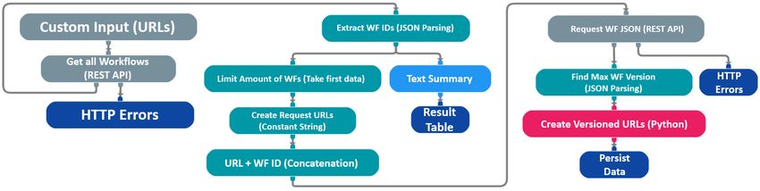
2      Wendlinger et al.

that needs to be managed properly - comparable to software artifacts in soft-
ware engineering [31]. A recently published case study from Amershi et al. [1]
showed the uptake of for example agile software engineering techniques for man-
aging ML workflows and identified also several hurdles. One hurdle originates
from knowledge sharing in a team developing ML workflows as well as the exper-
tise of the people themselves while a second hurdle clearly identified the need of
proper dataset management and a strict testing setup including hyper-parameter
optimization within a workflow. Overall, workflow management has to support
an highly iterative development process.
    In this work, we start from the hypothesis that the development of ML Work-
flows requires techniques like code completion, coverage analysis and testing
support, but focused on the particular properties of ML workflows. We therefore
develop semi-automated workflow recommendation and composition techniques
- based on Graph-Convolutional Neural Networks - for supporting development
teams in knowledge sharing and efficient workflow testing. More precisely, we
make the following contributions:
1. We analyze a large dataset of real-world data-science workflows consisting
   of 815 unique workflows in a total of 16035 versions from very diverse in-
   dustrial data science scenarios. We analyze the workflows and show that a
   large portion of the components relate to data wrangling and pre-processing,
   rather than to algorithmic aspects.
2. We define three tasks for semi-automatically supporting the management
   of ML workflows, namely finding similar workflows, suggesting and refining
   components as well as structure-based performance prediction. While the
   former two support ML engineers in workflow creation and composition, the
   latter improves hyper-parameter tuning efficiency and reduces testing time.
3. We develop baseline graph-level feature set for representing ML workflows
   and develop a Graph-Convolutional Network dubbed P-GCN exploiting ver-
   sion history of workflows in order to represent workflows and enable com-
   ponent suggestion and refinement. Contrary to much of the existing work
   based on graph embeddings (c.f. the survey [32]), we consider heterogeneous
   node properties and edge directions in workflows.
    We show that the P-GCN can produce high-quality dense representations
that preserve the inherent structure of the dataset. Furthermore, we demon-
strate that the P-GCN can learn complex mappings on DAG data by applying
it to structural performance prediction on NAS-Bench-101. In this task, it out-
performs state-of-the-art methods. Thirdly, it can be used to refine and suggest
components using an internal hybrid node- and graph-level representation and
thereby outperforms a strong baseline in both tasks.
    In the following, we give a detailed motivation and definition for the sup-
ported tasks in section 2 and go over related work in section 3. Our P-GCN
model is defined in 4 and section 5 lists the used datasets as well as relevant
qualities. We design experiments and present results for workflow similarity in
section 6, for structural performance prediction in section 7 and, finally, for
component refinement and suggestion in section 8.
Methods for Automatic Machine-Learning Workflow Analysis          3

   Source code including all experimental setups with results as well as datasets
are made available for reproduciblity.

2   Problem Definition

The creation, maintenance and management of ML workflows requires a powerful
descriptive framework such as the ONE DATA platform. Versioning and tracking of
results is especially important for efficient and reproducible work. Such a system,
in turn, lends itself to the creation of a workflow library that can be a useful
resource itself. To effectively leverage this resource, methods for the automatic
processing of workflows are needed. In the following, we present concepts that
can lead to improvements in three key areas.

Workflow Similarity Considering similar workflows can help developers in
reusing existing work and knowledge. Finding such workflows remains difficult. In
contrast to explicit meta-information for describing a workflow, grouping based
on structure alone does not require extra time on the user side and is more
general. However, the space of graph definitions is very high-dimensional and
sparse, making most distance measures defined over it meaningless and hard to
interpret. Another challenge is that graphs are a variable length structure, while
for most similarity calculations fixed length representations are required.
    A common approach to solving this problem is the transformation to a dense
lower-dimensional representation space. Between such representations, meaning-
ful distances can be computed and used for grouping. Such representations can
also be used as features for performance prediction or other meta-learning tasks.

Component Refinement and Suggestion Another useful tool in the design
of workflows is the automatic suggestion of components for a workflow. More
specifically, a model is to predict the best fitting component type for a node in a
workflow. This decision is based on patterns learned from a corpus of workflows
created by experts. Therefore, it can be formulated as a many-class classification,
a supervised learning task.
   Two scenarios can be differentiated, depending on how much information
about the rest of the workflow is available at prediction time. In Component
Suggestion, only the nodes ancestral to the considered node are known and, con-
sequently, at training time its decedents are artificially removed. For Component
Refinement, the whole workflow is available, except for information about the
considered node.

Structural Performance Prediction Performance prediction on DAGs can
be useful in both manual and automated search. It allows for focus on promising
instances and thereby makes the search more efficient. A reliable performance
predictor can reduce the number of costly executions for evaluation while keep-
ing regret low. The most useful predictors use only structural information and
therefore do not necessitate execution of the architecture.
4 Wendlinger et al.
This is especially useful for Neural Architecture Search (NAS) as each eval-
uation corresponds to full training with back propagation on a test dataset and
is therefore computationally expensive.
3 Related Work
Workflow Management There are many systematic approaches to the design
and management of user-defined processing workflows [3], [17], [12]. However,
despite the availability of workflow repositories and collection, they remain un-
derused for most methods that automate parts of the workflow creation process.
Friesen et al. propose the use of graph kernel, frequently occurring subgraphs
and paths for recommendation and tagging of bio-informatics processes in [7].
Graph Representations The main challenge in analyzing graph data is the
high dimensionality and sparsity of the representation. This poses problems for
manual analysis as well as for many automated methods designed for dense data.
Many algorithms for creating unsupervised node embeddings, a dense repre-
sentation that preserves distance-based similarity, have been devised to solve this
problem. Basic algorithms such as Adamic Adar [18] or Resource Allocation [34]
use local node information only.
DeepWalk [23] is the first deep learning approach to network analysis and
takes inspiration from methods for word embedding generation, such as Word2vec
[20]. Representations are learned on random walks that preserve the context of
a node and can be used for supervised learning tasks such as node classification.
Graph2vec [21] is a modification of document embedding models that pro-
duces whole graph embeddings by considering subgraph co-occurrence. How-
ever, it does not use edge direction which incurs significant data loss if applied
to workflow DAGs.
Graph Classification Graph Convolutional Networks were introduced by Kipf
et al. in [15]. They capture the neighborhood of a node through convolutional
filters, related to those known from Convolutional Neural Networks for images.
Shi et al. [26] construct a GCN based neural network assessor that uses a
global node to obtain whole-graph representations.
Tang et al. construct a relational graph for similarities between graphs based
on representations learned in an unsupervised manner through an auto-encoder
in [29]. A GCN regressor is fed this information and produces performance pre-
dictions for each input graph.
Lukasik et al. propose smooth variational graph embeddings for neural ar-
chitecture search in [19]. They are based on an autoencoder neural network in
which both the decoder and encoder consider the backward pass and the forward
pass of an architecture.
Ning et al. propose GATES in [22], a generic encoding scheme that uses
knowledge of the underlying search space with an attention mechanism for struc-
tural performance prediction in Neural Architecture Search. It is suitable for
both node-heterogeneous and edge-heterogeneous graph data.Methods for Automatic Machine-Learning Workflow Analysis 5
4 Residual Graph-Level Graph Convolutional Networks
In this section, we introduce our graph convolutional model dubbed P-GCN that
offers a robust aggregation method for whole-graph representation learning and
related supervised tasks. We also go over the basics of graph convolutions and
adjacent techniques used for P-GCN.
Graph Convolutional Networks [15] can be used to compute node-level func-
tions. They take the graph structures and node features as input. These features
may be one-hot encoded node types or any other type of feature such as more
detailed node hyper-parameters. Similar to convolutions in image recognition,
multiple learned filters are used to aggregate features from neighboring nodes via
linear combination. Quite like CNNs, GCNs derive their expressive power from
the stacking of multiple convolution layers that perform increasingly complex
feature extraction based on the previous layers’ output. Usually, a bottleneck
is created by stacking multiple layers and adding a smaller last convolutional
layer. This forces the model to compress information and create a denser and
more meaningful representation of size FL .
Formally, we consider ML workflows as heterogeneous directed acyclic graph
(DAG) representing the data flow between different data processing compo-
nents. Specifically, G = (V, E, λl ) represents a graph with nodes (or vertices) V
and edges E ⊆ {(u, v) : u, v ∈ V ∧ u 6= v}. A mapping λ : V → {0, 1}nl assigns
a one-hot-encoded label, or node type, to each node. E expresses data flow be-
tween nodes while the node class λ(v) is the kind of data processing component
that v represents, of a total nl possible component types.
A graph convolution in layer ` of L layers with filter size F` on node v of G
is defined as
(`+1)
X
fi (G, v) = Θ(`+1) f (`) (G, u)z(v) (1)
u∈Γi (G,v)
(`) (`+1)
with a layer weight matrix Θ(`+1) ∈ RF ×F and i = 1. Γi (G, v) is
the ith neighborhood of v w.r.t. G and z(u) is a normalization, usually the
inverse square root of the node degrees. Self-loops are added artificially to G
(`+1)
as E = E ∪ {(u, v) : v ∈ V} so the representation fi (G, v) also contains
(`)
fi (G, v). For the first layer, the input features are used as node representations,
i.e. f (0) (G, v) = λl (v) and F (0) = nl .
Topology adaptive GCNs [6] are an extension of the graph convolution that
considers neighborhoods of hop sizes up to k. This changes the convolution in
layer ` to
(`+1) (`)
X
f (`+1) (G, v) = Θi fi (G, v)z(v) (2)
i∈{1..k}
` `+1
with learned weights Θ(`+1) ∈ RkF ×F for each layer. We adopt this
method with k set to 2 for its flexibility and improved expressive power.6 Wendlinger et al.
In this way, a GCN can generate meaningful node-level representations, i.e.
a FL sized representation for each v ∈ V. If we want graph-level outputs, i.e. one
embedding that encodes the structure of a whole graph, pooling can be used.
More specifically, we use a function gi : R|V |×FL → RFL to obtain a fixed-size
representation regardless of graph size. We can use a set G of pooling functions
such as mean, min, max or stdev for each embedding dimension for improved
robustness. This produces an output of size |G| × FL for each graph. These
pooling results are then scaled via batch normalization [10] and aggregated via
a weighted sum, resulting in an output of size FL :
X (L+1)
f (L+1) (G, gi ) = gi fi (G, v)
v∈V
X (L+1)
(3)
f (L+1) (G) = Θi Z f (L+1) (G, gi )
i∈{1..|G|}
L+1 L
with learned weights Θ(L+1) ∈ RF ×|G| F and normalization function Z.
For unsupervised tasks, f (L+1) (G) is the final model output. The model can
also be adapted to supervised tasks by adding dense layers that function like
an MLP estimator. For classification, a softmax -activated dense layer with the
appropriate number of outputs for the predicted classes can be added. For re-
gression, a dense layer with one output serves as the last layer.
To help convergence, batch normalization [10] is applied to each graph con-
volution’s output to reduce the co-variate shift during training. Furthermore,
Batch normalization after the pooling helps reduce the impact of different scales
induced by the different pooling operations. According to the Ioffe et al., they
also provide some regularization. This also means that convolutional layers that
are followed by a batch normalization do not require a learned bias, as their
output is scaled to zero mean anyway.
Skip connections as introduced by He et al. in [8] are automatically added
between layers of matching size so residuals can be learned explicitly, which can
help deeper architectures converge and generally improve performance, c.f. [5].
This changes the feature computation to
( (`−1)
(`+1) σ f (`+1) (G) + fres (G) if F (`−1) = F (`+1)
fres (G) = (4)
σ f (`+1) (G) otherwise
with a non-linear activation function σ : R → R, rectification in our case. In
the same vein, a dropout layer [9] is added after the last graph convolution to
obtain a model that generates more robust representations.
P-GCN is trained in mini-batches with adaptive momentum [14] and expo-
nential learning rate decay. As over-fitting can be a problem in complex settings,
weight decay is applied automatically with a factor of 0.01.
5 Datasets
This section introduces the datasets used to develop and validate our methods.Methods for Automatic Machine-Learning Workflow Analysis 7
The ONE DATA data science workflow dataset ODDS-full2 comprises 815 unique
workflows in temporally ordered versions obtained from a broad range of real-
world machine learning solutions realized using the ONE DATA platform. Conse-
quently, the data set distinguishes itself from available academic datasets, espe-
cially when analyzing potential ML workflow support for real-world applications.
A version of a workflow describes its evolution over time, so whenever a workflow
is altered meaningfully, a new version of this respective workflow is persisted.
Overall, 16 035 versions are available.
ODDS workflows represent machine learning workflows expressed as node-
heterogeneous DAGs with 156 different node types. They can represent a wide
array of data science and machine learning tasks with multiple data sources,
model training, model inference and data munging. These node types represent
various kinds of processing steps of a general machine learning workflow and are
grouped into 5 broad categories, which are listed below.
Load Processors for loading or generating data (e.g. random number generator).
Save Processors for persisting data (possible in various data formats, via exter-
nal connections or as a contained result within the ONE DATA platform) or
for providing data to other places as a service.
Transformation Processors for altering and adapting data. This includes e.g.
database-like operations such as renaming columns or joining tables as well
as fully fledged dataset queries.
Quantitative Methods Various aggregation or correlation analysis, bucket-
ing, and simple forecasting.
Advanced Methods Advanced machine learning algorithms such as BNN or
Linear Regression. Also includes special meta processors that for example
allow the execution of external workflows within the original workflow.
An example workflow is shown in Figure 1. Any metadata beyond the struc-
ture and node types of a workflow has been removed for anonymization purposes.
Fig. 1. Example Workflow used in the ONE DATA platform.
ODDS, a filtered variant, which enforces weak connectedness and only con-
tains workflows with at least 5 different versions and 5 nodes, is available as the
default version for unsupervised and supervised learning.
2
Available at https://zenodo.org/record/46337048 Wendlinger et al.
Statistic ODDS-full ODDS NAS-Bench-101 [33]
unique workflows 815 284 423k
instances 16035 8639 1.27M
node types 156 121 5
mean graph size 42.78±63.27 57.21±69.34 8.73±0.55
Table 1. Statistics for the full and filtered ONE DATA data science workflow datasets
as well as NAS-Bench-101.
As a second data set we use NAS-bench-101 [33], which was published as
a benchmark dataset for Neural-Architecture-Search (NAS) and NAS meta-
learning. It consists of architectures sampled from a common search space fo-
cusing on standard machine learning tasks. These represent cells constructed of
high-level CNN operations from which CNNs are generated by stacking them
with a fixed strategy. 423k such architectures were trained with the same back-
propagation schema on the image recognition task CIFAR-10 [16]. We use their
accuracies in this task as our prediction target. Consequently, this can be seen
as a sampling of generalization power for neural architectures and is therefore
well suited for structural performance prediction.
6 Workflow Similarity
In the following, we will describe different approaches for creating dense repre-
sentations from heterogeneous DAGs, starting with simple graph features and
ending with deep-learning methods with the aim to detect similar workflows.
Evaluation Methodology As learning such representations is an unsupervised
task, quantitative evaluation is difficult. However, the structure imposed by the
version groups of ODDS enables the definition of two informative criteria. One of
those, dubbed the Group Cluster Score, indicates how well the embeddings are
suited to clustering tasks. This is done by generating a clustering and evaluating
how well it represents the workflow groups. Agglomerative clustering via Ward
linkage [11] was chosen for this task due to its robustness and determinism. The
V-Measure [24], defined as the harmonic mean of homogeneity and completeness,
of this clustering is reported as the GCS.
Furthermore, the Triplet Ratio Score indicates how closely instances of a
workflow group are embedded together. It is defined as the mean of the dis-
tance to positive instances divided by the distance to negative instances for each
sample. Consequently, lower triplet ratio scores are better.
Results Simple graph features can be used to group workflows. Some of them
are computed on the graph-level, such as the number of nodes or number of
edges. Others, such as centrality measures, are extracted on the node-level and
can be aggregated via their mean or other statistical moments. In the case of
heterogeneous graphs, they can require significant manual feature engineering toMethods for Automatic Machine-Learning Workflow Analysis 9
respect the different node types. Furthermore, they do not produce a generally
dense representation, as certain features can be sparse for some classes of DAGs.
As a compromise, we choose to use the feature set presented in [27] and
extend them with the number of distinct node types in the graph and the count
of nodes for the most frequent node type.
Graph Convolutional Networks have been shown to create meaningful em-
beddings on some data without training, c.f. [15]. However, we can use methods
for learning on grouped data to generate useful embeddings. For this method,
distinct workflows can be regarded as groups with their versions representing
members of those groups. A P-GCN model can be trained to minimize the dis-
tance within groups while maximizing the distance to members of other groups.
This can be achieved via triplet loss. Triplet loss is calculated on triplets of
samples, where the current sample is the so-called anchor. Based on the group
of this anchor, a positive instance from the same group as well as a negative
instance from another group are sampled. Triplet loss can be computed either
based on the ranking of these samples or on the ratio between their distances.
Triplet margin loss, as described in [30], is a ranking loss that forces the model
to embed anchor and positive closer together than anchor and negative.
Approach GCS TRS
Graph2Vec [21] 0.596±0.0045 0.453±0.0039
FeatherGraph [25] 0.76 0.351
Basic graph-level Features 0.701 0.339
Untrained P-GCN 0.884±0.0013 0.4±0.0069
Triplet margin loss P-GCN 0.901±0.0038 0.113±0.0032
Table 2. Representation quality for different methods on ODDS. For non-deterministic
models, mean and standard deviation across 5 trials with different random states are
given.
As can be seen in Table 2, P-GCN trained with triplet margin loss produces
high-quality representations for the high-dimensional data of ODDS. They have
both significantly better GCS as well as TRS scores compared to traditional
approaches that cannot natively use directed or heterogeneous graphs. Interest-
ingly, embeddings generated with an untrained, fully random P-GCN achieve
competitive GCS scores with relatively high repeatability.
Hyper-parameters are given in Table 3. P-GCN benefits from large mini-
batches and high exponential learning rate decay in this task to achieve smoother
convergence behavior.
7 Structural Performance Prediction
For predicting workflow performance based on a workflow structure, we adapted
the P-GCN model towards a regression task by adding fully connected layers10 Wendlinger et al.
Parameter Name Default Value
GCN Layer Sizes (128, 128, 128, 128, 128, 64)
Pooling Operations (max, min, mean, stdev)
Epochs 50
Dropout Probability 0.05
Batch Size 1000
Learning Rate 0.01
Learning Rate Decay 0.9
Table 3. P-GCN parameter setting for unsupervised learning on ODDS.
with non-linearities after the graph convolutions. These function like an MLP
regressor after the GCN-based feature extraction, but are trained jointly. Layer
Normalization as per Ba et al. [2] is applied to the output of each dense layer for
improved convergence behavior.
We use a combined loss, a linear combination of MSE loss and hinge pairwise
ranking loss as defined in [22]. For true accuracy y and prediction ŷ of length N
and margin m = 0.05:
Lc (y, ŷ) = w1 · M SE(y, ŷ) + w2 · Lr (y, ŷ)
N
X X (5)
Lr (y, ŷ) = max (0, m − (ŷi − ŷj ))
j=1 i: yi >yj
A focus on low squared error or high ranking correlation can be facilitated
through the respective weights w1 and w2 . This is important since we found that
many low-error predictions have low correlation and vice-versa.
Nl Parameter Parameter Name Default Value
1000 Dense layer sizes (64, )
Training epochs 150
Learning rate decay 0.95
w1 MSE loss weight 0.5
w2 Hinge ranking loss weight 0.5
Batch size 100
381 Batch size 50
1906 Batch size 200
Table 4. Parameter Setting for the P-GCN for supervised learning on NAS-Bench-101.
All other hyper-parameters are set as before, c.f. Table 3.
Analogous to the method of Lukasik et al. in [19], the back-propagation used
in the training of ANNs can be considered by reversing the edge direction of an
individual architecture. The predictor is presented both versions and produces
a single prediction. P-GCN does this by jointly aggregating over the node-level
representations of both passes.Methods for Automatic Machine-Learning Workflow Analysis 11
Evaluation Methodology The specific architectures in the training set can
have a large impact on predictor performance. Therefore multiple trials with
different dataset splits, 5 in our case, need to be performed for proper evaluation.
The remaining instances are randomly partitioned into Nl training instances and
a test set of size 50 000 for each fold. For each of these trials, the pseudo-random
number generator used for initialization of network parameters is used with a
different seed as well. This setup enables us to assess repeatability.
As this is a regression task, multiple metrics can be use to quantitatively
evaluate predictions. Mean squared error alone is unsuitable as it is difficult
to interpret and can be low for meaningless predictions. In most searches, per-
formance predictions are only compared with other predictions. It is therefore
not important that they exhibit low error with the target, but rather that they
show high correlation with the target. Furthermore, as many search methods
rank candidates by performance, ranking correlation can be considered the most
important measure.
Concordant with [29], we choose mean squared error, Pearson correlation ρp
and the Kendall Tau ranking coefficient τk [13] as evaluation criteria.
Results Performance prediction was performed on NAS-bench-101 [33]. Results
for 5 random folds are listed in Table 5. Our method offers improvements over
state of the art methods with respect to the most important ranking correlation
τk . This is despite the fact that P-GCN is a purely supervised method and does
not need any information beyond the Nl training instances.
Nl Criterion SVGe[19] GCN[26] Tang et al. [29] GATES[22] P-GCN (Ours)
381 τk - - - 0.7789 0.7985±0.008
1000 τk - - 0.6541±0.0078 - 0.8291±0.0.0067
MSE 0.0028±0.00002 - 0.0031±0.0003 - 0.0038±0.0.00016
ρp - 0.819 0.5240±0.0068 - 0.589±0.024
1906 τk - - - 0.8434 0.8485±0.0013
Table 5. Performance prediction results on NAS-Bench-101 with Nl training instances.
Mean and standard deviation over 5 random trials for multiple evaluation criteria.
Figure 2 offers a more detailed look at the predictions for one fold. There is a
strong linear relationship, but also a bias resulting from the used combined loss.
By altering the loss weights w1 and w2 , the focus can be shifted towards one
of the two prediction goals - low error or high correlation. The corresponding
predictive performance can be observed in Figure 3. The default configuration
with equally weighted losses does not impair performance w.r.t. to τk . Optimizing
P-GCN purely for MSE produces predictions with a MSE of 0.00206±0.00009 ,
which is an improvement over the state of the art, SVGe’s 0.0028±0.00002 .12 Wendlinger et al.
Fig. 2. P-GCN performance predictions for 50 000 test instances from a single fold
with Nl = 1 000. Comparison of performance values (left) and rankings (right) with
corresponding correlations, i.e. Pearson and Spearman coefficient, given.
8 Component Refinement and Suggestion
For component refinement, a set of basic numeric features can be extracted
from the complex workflow structures to form a baseline. To this end, we use
the same graph-level and node-level features employed for workflow similarity
computation (c.f. section 6), based on the set constructed in [27]. However, for
this task, the node-level centrality measures are not aggregated. Furthermore,
they are supplemented with harmonic centrality, pagerank, load centrality and
katz centrality. For obvious reasons, node betweenness centrality is used instead
of edge betweenness centrality. Additionally, the number of descendents and
ancestors of each node as well as the longest shortest path to and from each node
are added to provide explicit information about its position in the workflow.
The P-GCN model can be adapted to this task. To produce a joint rep-
resentation of both the considered node and the workflow it is part of, their
representations are concatenated. More precisely, the node representation is ap-
pended to the outputs of the pooling functions. This is fed into an MLP like the
one used for structual performance prediction, c.f. section 7. A softmax-activated
output layer with a neuron for each class is added and the network’s categorical
cross-entropy loss is optimized via back-propagation. Due to the larger training
set sizes, small alterations to the training schema were necessary, c.f. Table 6.
Parameter Default Value
Epochs 50
Loss categorical cross-entropy
Dropout 0.25
Batch Size 5000
Table 6. Parameter Setting for the hybrid P-GCN for node-level classification on
ODDS. All other hyper-parameters are set as before, c.f. Table 4.Methods for Automatic Machine-Learning Workflow Analysis 13
Fig. 3. P-GCN performance on NAS-bench-101 in response to varying MSE loss weight
w1 for the combined loss function. Shown with ± stdev confidence intervals across 5
folds. The hinge ranking loss weight w2 is set to 1 − w1 .
The hybrid P-GCN constructed such can utilize both information about the
considered node as well as its workflow, extracted through the same graph con-
volutional functions. This removes the need for manually engineered and hard
to generalize graph-level features that capture this node context.
Evaluation Methodology In an application case, we can expect a component
refinement model to be applied to unseen workflows only, i.e. such that differ
from those in the training set. To obtain a realistic evaluation with respect to
this use case, multiple grouped splits are used. The data set is split into a certain
percentage of groups for training while the rest is withheld for testing. For this
task, the groups are created by the distinct workflows. 5 splits with 80% of groups
used for training and the rest withheld for testing are created in this way.
For component suggestion we only consider nodes with at least 5 ancestors
to guarantee a minimum level of information available for the prediction.
As this prediction tasks requires inference for every single node of every
graph, the computational load is very high. This can be remedied by removing
very similar instances, i.e. by sub-sampling over the version history with a factor
of 10, starting with the newest revision. As a result, only every 10th version of
a workflow is present in the data-set used for training and testing.
Results Various classifiers were tested on the basic feature set. Many of these
are superior to the dummy classifier baseline, c.f. Table 7. The best performing
method is a random forest classifier [4]. The hybrid P-GCN with slightly adapted
hyper-parameters, c.f. Table 6, outperforms the basic methods in both tasks.
While graph-level P-GCN achieves competitive results in component refine-
ment and node-level P-GCN performs well in component suggestion, neither ap-14 Wendlinger et al.
Component Refinement Component Suggestion
classifier accuracy top 5 accuracy accuracy top 5 accuracy
Dummy Classifier 0.245±0.063 0.452±0.025 0.179±0.02 0.527±0.051
Random Forest 0.553±0.07 0.744±0.047 0.461±0.078 0.715±0.067
Node-level P-GCN 0.442±0.08 0.758±0.061 0.48±0.059 0.755±0.06
Graph-level P-GCN 0.578±0.041 0.759±0.028 0.27±0.043 0.584±0.062
Hybrid P-GCN 0.643±0.074 0.798±0.046 0.461±0.08 0.748±0.06
Table 7. Performance comparison for component refinement and component sugges-
tion in 5 random grouped folds. Results for P-GCNs and a set of different classifiers
using basic graph features.
proach excels in both tasks. The hybrid P-GCN however can deliver high quality
prediction in both scenarios, showing that it is a best-of-both-worlds approach.
In component refinement, it achieves a mean accuracy 0.643 ± 0.074 and a
mean Top-5-accuracy 0.798 ± 0.046. This means that, on average, for 4 out of
5 nodes, the correct component type can be found in the top 5 predictions and
for 5 out of 8 nodes the prediction is correct.
Despite the limitation to nodes with at least 5 ancestors, component sug-
gestion is a distinctly more challenging task. However, P-GCN methods still
outperform the strong random forest baseline by a significant margin.
9 Conclusion
The management and analysis of real-world ML workflows poses a number of
interesting challenges, most prominently the generation of meaningful represen-
tations and component refinement. For both tasks, a baseline with adequate
performance is presented and evaluated on the ODDS dataset.
P-GCN is a modification of node-level topology adaptive GCNs that shows
promise for supervised tasks as well as unsupervised tasks with surrogate tar-
gets. It can generate meaningful representations for the highly complex data
structures of ODDS and outperforms the state of the art in NAS-Bench-101
performance prediction. Additionally, it can be configured to create joint node-
and graph-level representations and thereby outperforms a strong baseline in a
node classification task on ODDS.
Since P-GCN is used in a purely supervised manner for regression tasks, it
does not require a large-scale sampling or rule-based definition of the search
space for generating unsupervised representations, as other methods do. The
pooling method also makes it suitable for search spaces with varying graph
sizes. Furthermore, input node features can easily be extended to cover node
hyper-parameters or arbitrary numerical attributes. These properties make the
adaptation of P-GCN to other performance prediction tasks trivial. Especially
the predictive performance on supervised tasks with more complex and varied
DAGs, such as those generated by CGP-CNN [28], would provide further insight
into the capabilities of the model. P-GCN’s generality also makes it an interestingMethods for Automatic Machine-Learning Workflow Analysis 15
candidate for transductive transfer as well. Multiple domains with information
processing expressed in DAG architectures are worth considering.
Acknowledgments This work has been partially funded by the Bavarian Min-
istry of Economic Affairs, Regional Develoment and Energy under the grant
’CrossAI’ (IUK593/002) as well as by BMK, BMDW, and the Province of Up-
per Austria in the frame of the COMET Programme managed by FFG. It was
also supported by the FFG BRIDGE project KnoP-2D (grant no. 871299).
References
1. Amershi, S., Begel, A., Bird, C., DeLine, R., Gall, H., Kamar, E., Nagappan,
N., Nushi, B., Zimmermann, T.: Software engineering for machine learning: A case
study. In: 2019 IEEE/ACM 41st International Conference on Software Engineering:
Software Engineering in Practice (ICSE-SEIP). pp. 291–300. IEEE (2019)
2. Ba, J.L., Kiros, J.R., Hinton, G.E.: Layer normalization. arXiv preprint
arXiv:1607.06450 (2016)
3. Basu, A., Blanning, R.W.: A formal approach to workflow analysis. Information
Systems Research 11(1), 17–36 (2000)
4. Breiman, L.: Random forests. Machine learning 45(1), 5–32 (2001)
5. Bresson, X., Laurent, T.: Residual gated graph convnets. arXiv preprint
arXiv:1711.07553 (2017)
6. Du, J., Zhang, S., Wu, G., Moura, J.M., Kar, S.: Topology adaptive graph convo-
lutional networks. arXiv preprint arXiv:1710.10370 (2017)
7. Friesen, N., Rüping, S.: Workflow analysis using graph kernels. In: LWA. pp. 59–66.
Citeseer (2010)
8. He, K., Zhang, X., Ren, S., Sun, J.: Deep residual learning for image recognition. In:
Proceedings of the IEEE conference on computer vision and pattern recognition.
pp. 770–778 (2016)
9. Hinton, G.E., Srivastava, N., Krizhevsky, A., Sutskever, I., Salakhutdinov, R.R.:
Improving neural networks by preventing co-adaptation of feature detectors. arXiv
preprint arXiv:1207.0580 (2012)
10. Ioffe, S., Szegedy, C.: Batch normalization: Accelerating deep network training by
reducing internal covariate shift. arXiv preprint arXiv:1502.03167 (2015)
11. Jr., J.H.W.: Hierarchical grouping to optimize an objective function. Jour-
nal of the American Statistical Association 58(301), 236–244 (1963).
https://doi.org/10.1080/01621459.1963.10500845
12. Kaushik, G., Ivkovic, S., Simonovic, J., Tijanic, N., Davis-Dusenbery, B., Deniz,
K.: Graph theory approaches for optimizing biomedical data analysis using repro-
ducible workflows. bioRxiv p. 074708 (2016)
13. Kendall, M.G.: A new measure of rank correlation. Biometrika 30(1/2), 81–93
(1938)
14. Kingma, D.P., Ba, J.: Adam: A method for stochastic optimization. arXiv preprint
arXiv:1412.6980 (2014)
15. Kipf, T.N., Welling, M.: Semi-supervised classification with graph convolutional
networks. arXiv preprint arXiv:1609.02907 (2016)
16. Krizhevsky, A., Hinton, G., et al.: Learning multiple layers of features from tiny
images (2009)16 Wendlinger et al.
17. Li, J., Fan, Y., Zhou, M.: Timing constraint workflow nets for workflow analy-
sis. IEEE Transactions on Systems, Man, and Cybernetics-Part A: Systems and
Humans 33(2), 179–193 (2003)
18. Liben-Nowell, D., Kleinberg, J.: The link-prediction problem for social networks.
Journal of the American society for information science and technology 58(7),
1019–1031 (2007)
19. Lukasik, J., Friede, D., Zela, A., Stuckenschmidt, H., Hutter, F., Keuper, M.:
Smooth variational graph embeddings for efficient neural architecture search. arXiv
preprint arXiv:2010.04683 (2020)
20. Mikolov, T., Sutskever, I., Chen, K., Corrado, G.S., Dean, J.: Distributed repre-
sentations of words and phrases and their compositionality. Advances in neural
information processing systems 26, 3111–3119 (2013)
21. Narayanan, A., Chandramohan, M., Venkatesan, R., Chen, L., Liu, Y., Jaiswal,
S.: graph2vec: Learning distributed representations of graphs. arXiv preprint
arXiv:1707.05005 (2017)
22. Ning, X., Zheng, Y., Zhao, T., Wang, Y., Yang, H.: A generic graph-based neural
architecture encoding scheme for predictor-based nas (2020)
23. Perozzi, B., Al-Rfou, R., Skiena, S.: Deepwalk: Online learning of social represen-
tations. In: Proceedings of the 20th ACM SIGKDD international conference on
Knowledge discovery and data mining. pp. 701–710 (2014)
24. Rosenberg, A., Hirschberg, J.: V-measure: A conditional entropy-based external
cluster evaluation measure. In: Proceedings of the 2007 joint conference on empir-
ical methods in natural language processing and computational natural language
learning (EMNLP-CoNLL). pp. 410–420 (2007)
25. Rozemberczki, B., Sarkar, R.: Characteristic functions on graphs: Birds of a feather,
from statistical descriptors to parametric models (2020)
26. Shi, H., Pi, R., Xu, H., Li, Z., Kwok, J.T., Zhang, T.: Multi-objective neural
architecture search via predictive network performance optimization (2019)
27. Stier, J., Granitzer, M.: Structural analysis of sparse neural networks. Procedia
Computer Science 159, 107–116 (2019)
28. Suganuma, M., Shirakawa, S., Nagao, T.: A genetic programming approach to
designing convolutional neural network architectures. In: Proceedings of the genetic
and evolutionary computation conference. pp. 497–504 (2017)
29. Tang, Y., Wang, Y., Xu, Y., Chen, H., Shi, B., Xu, C., Xu, C., Tian, Q., Xu, C.: A
semi-supervised assessor of neural architectures. In: Proceedings of the IEEE/CVF
Conference on Computer Vision and Pattern Recognition. pp. 1810–1819 (2020)
30. Vassileios Balntas, Edgar Riba, D.P., Mikolajczyk, K.: Learning local feature de-
scriptors with triplets and shallow convolutional neural networks. In: Richard
C. Wilson, E.R.H., Smith, W.A.P. (eds.) Proceedings of the British Machine
Vision Conference (BMVC). pp. 119.1–119.11. BMVA Press (September 2016).
https://doi.org/10.5244/C.30.119, https://dx.doi.org/10.5244/C.30.119
31. Weißgerber, T., Granitzer, M.: Mapping platforms into a new open science model
for machine learning. it-Information Technology 61(4), 197–208 (2019)
32. Wu, Z., Pan, S., Chen, F., Long, G., Zhang, C., Philip, S.Y.: A comprehensive
survey on graph neural networks. IEEE Transactions on Neural Networks and
Learning Systems (2020)
33. Ying, C., Klein, A., Christiansen, E., Real, E., Murphy, K., Hutter, F.: Nas-bench-
101: Towards reproducible neural architecture search. In: International Conference
on Machine Learning. pp. 7105–7114. PMLR (2019)
34. Zhou, T., Lü, L., Zhang, Y.C.: Predicting missing links via local information. The
European Physical Journal B 71(4), 623–630 (2009)You can also read