Teaching 3D Geometry to Deformable Part Models
←
→
Page content transcription
If your browser does not render page correctly, please read the page content below
Teaching 3D Geometry to Deformable Part Models
Bojan Pepik1 Michael Stark1,2 Peter Gehler3 Bernt Schiele1
1
Max Planck Institute for Informatics, 2 Stanford University, 3 Max Planck Institute for Intelligent Systems
Abstract
Current object class recognition systems typically target
2D bounding box localization, encouraged by benchmark
data sets, such as Pascal VOC. While this seems suitable
for the detection of individual objects, higher-level applica-
tions such as 3D scene understanding or 3D object tracking
would benefit from more fine-grained object hypotheses in-
corporating 3D geometric information, such as viewpoints
or the locations of individual parts. In this paper, we help
narrowing the representational gap between the ideal in-
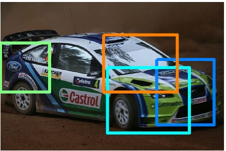
put of a scene understanding system and object class detec- Figure 1. Example detections of our DPM-3D-Constraints. Note
tor output, by designing a detector particularly tailored to- the correspondence of parts found across different viewpoints
wards 3D geometric reasoning. In particular, we extend the (color coded), achieved by a 3D parameterization of latent part
successful discriminatively trained deformable part models positions (left). Only five parts (out of 12 parts) are shown for
to include both estimates of viewpoint and 3D parts that are better readability.
consistent across viewpoints. We experimentally verify that titative geometric representations, where reasoning is typi-
adding 3D geometric information comes at minimal perfor- cally limited to the level of entire objects [18, 15, 33, 34].
mance loss w.r.t. 2D bounding box localization, but outper- The starting-point and main contribution of this paper
forms prior work in 3D viewpoint estimation and ultra-wide is therefore to leave the beaten path towards 2D BB pre-
baseline matching. diction, and to explicitly design an object class detector
with outputs amenable to 3D geometric reasoning. By bas-
ing our implementation on the arguably most successful 2D
1. Introduction BB-based object class detector to date, the deformable part
model (DPM [10]), we ensure that the added expressive-
Object class recognition has reached remarkable perfor- ness of our model comes at minimal loss with respect to
mance for a wide variety of object classes, based on the its robust image matching to real images. To that end, we
combination of robust local image features with statistical propose to successively add geometric information to our
learning techniques [12, 19, 10]. Success is typically mea- object class representation, at three different levels.
sured in terms of 2D bounding box (BB) overlap between First, we rephrase the DPM as a genuine structured out-
hypothesized and ground truth objects [8] favoring algo- put prediction task, comprising estimates of both 2D ob-
rithms implicitly or explicitly optimizing this criterion [10]. ject BB and viewpoint. This enables us to explicitly con-
At the same time, interpretation of 3D visual scenes in trol the trade-off between accurate 2D BB localization and
their entirety is receiving increased attention. Reminiscent viewpoint estimation. Second, we enrich part and whole-
of the earlier days of computer vision [23, 5, 26, 22], rich, object appearance models by training images rendered from
3D geometric representations in connection with strong ge- CAD data. While not being as representative as real images
ometric constraints are increasingly considered a key to suc- in terms of feature statistics, these images literally come
cess [18, 7, 15, 33, 34, 2, 16]. Strikingly, there is an apparent with perfect 3D annotations e.g. for position and viewpoint,
gap between these rich 3D geometric representations and which we can use to improve localization performance and
what current state-of-the-art object class detectors deliver. viewpoint estimates.
As a result, current scene understanding approaches are of- And third, we extend the notion of discriminatively
ten limited to either qualitative [15] or coarse-grained quan- trained, deformable parts to 3D, by imposing 3D geomet-
To appear in the Proc. of the IEEE Conf. on Computer Vision and Pattern Recognition (CVPR), Providence, Rhode Island, June 2012.
c 2012 IEEE. Personal use of this material is permitted. Permission from IEEE must be obtained for all other uses, in any current or future media, including
reprinting/republishing this material for advertising or promotional purposes, creating new collective works, for resale or redistribution to servers or lists, or
reuse of any copyrighted component of this work in other works.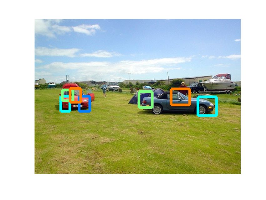
ric constraints on the latent positions of object parts. This    3D CAD models [20, 28] and point clouds from structure-
ensures consistency between parts across viewpoints (i.e.,       from-motion [35, 1, 13] or depth sensors [30], their out-
a part in one view corresponds to the exact same physical        puts are typically still limited to 2D BBs and associated
portion of the object in another view, see Fig. 1), and is       viewpoint estimates, conveying little information for fine-
achieved by parameterizing parts in 3D object coordinates        grained, geometric, scene-level reasoning. In contrast, our
rather than in the image plane during training. This con-        method outputs additional estimates of latent part positions
sistency constitutes the basis of both reasoning about the       that are guaranteed to be consistent across viewpoints, and
spatial position of object parts in 3D and establishing part-    can therefore be used to anchor part-level correspondences,
level matches across multiple views. In contrast to prior        thereby providing strong scene-level constraints. While this
work based on 3D shape [28, 36], our model learns 3D vol-        is similar in spirit to the SSfM approach of [2], we aim at
umetric parts fully automatically, driven entirely by the loss   fine-grained reasoning on the level of parts rather than en-
function.                                                        tire objects. We note that the depth-encoded Hough voting
    In an experimental study, we demonstrate two key prop-       scheme of [30] outputs depth estimates for individual fea-
erties of our models. First, we verify that the added ex-        tures, but does not report quantitative results on how con-
pressive power w.r.t accurate object localization, viewpoint     sistently these features can be found across views. On the
estimation and 3D object geometry does not hurt 2D de-           other hand, we outperform the detailed PCA shape model
tection performance too much, and even improves in some          of [36] in an ultra-wide baseline matching task.
cases. In particular, we first show improved performance of          On the technical side, we observe that multi-view recog-
our structured output prediction formulation over the origi-     nition is often phrased as a two step procedure, where object
nal DPM for 18 of 20 classes of the challenging Pascal VOC       localization and viewpoint estimation are performed in suc-
2007 data set [9]. We then show that our viewpoint-enabled       cession [24, 20, 13, 36]. In contrast, we formulate a coher-
formulation further outperforms, to the best of our knowl-       ent structured output prediction task comprising both, and
edge, all published results on 3D Object Classes [27].           simultaneously impose 3D geometric constraints on latent
    Second, we showcase the ability of our model to de-          part positions. At the same time, and in contrast to the
liver geometrically more detailed hypotheses than just 2D        part-less mixture of templates model by [14], we benefit
BBs. Specifically, we show a performance improvement             from the widely recognized discriminative power of the de-
of up to 8% in viewpoint classification accuracy compared        formable parts framework. To our knowledge, our paper
to related work on 9 classes of the 3D Object Classes data       is the first to simultaneously report competitive results for
set. We then exploit the consistency between parts across        2D BB prediction, 3D viewpoint estimation, and ultra-wide
viewpoints in an ultra-wide baseline matching task, where        baseline matching.
we successfully recover relative camera poses of up to 180
degrees spacing, again improving over previous work [36].        2. Structured learning for DPM
                                                                    In the following, we briefly review the DPM model [10]
Related work. 3D geometric object class representations          and then move on to the extensions we propose in order to
have been considered the holy grail of computer vision           “teach it 3D geometry”. For comparability we adopt the
since its early days [23, 5, 26, 22], but proved difficult to    notation of [10] whenever appropriate.
match robustly to real world images. While shape-based
incarnations of these representations excel in specific do-      2.1. DPM review
mains such as facial pose estimation [3] or markerless mo-           We are given training data {(Ii , yi )}1,...,N where I de-
tion capture, they have been largely neglected in favor of       notes an image and y = (y l , y b ) ∈ Y is a tuple of image
less descriptive but robust 2D local feature-based represen-     annotations. The latter consists of y b , the BB position of
tations for general object class recognition [12, 19, 10].       the object, e.g. specified through its upper, lower, left and
    Only recently, the 3D nature of objects has again            right boundary, and y l ∈ {−1, 1, . . . , C} the class of the
been acknowledged for multi-view object class recognition,       depicted object or −1 for background.
where an angular viewpoint is to be predicted in addition to         A DPM is a mixture of M conditional random fields
a 2D object BB. Many different methods have been sug-            (CRFs). Each component is a distribution over object hy-
gested to efficiently capture relations between the object       potheses z = (p0 , . . . , pn ), where the random variable
appearance in different viewpoints, either by feature track-     pj = (uj , vj , lj ) denotes the (u, v)-position of an object part
ing [31], image transformations [1], or probabilistic view-      in the image plane and a level lj of a feature pyramid image
point morphing [29], and shown to deliver remarkable per-        features are computed on. The root part p0 corresponds to
formance in viewpoint estimation.                                the BB of the object. For training examples we can iden-
    While several approaches have successfully demon-            tify this with y b , whereas the parts p1 , . . . , pn are not ob-
strated the integration of 3D training data in the form of       served and thus latent variables. We collect the two latent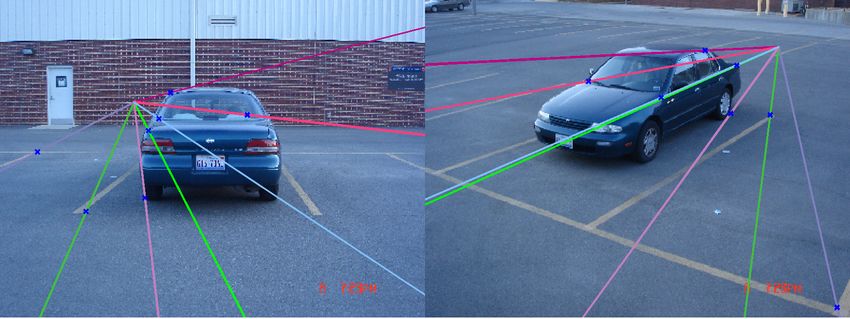
variables of the model in the variable h = {c, p1 , . . . , pn },         effect to include the two constraint sets of problem (1) into
where c ∈ {1, . . . , M } indexes the mixture component.                  this optimization program.
    Each CRF component is star-shaped and consists of                         Based on the choice of ∆ we distinguish between the
unary and pairwise potentials. The unary potentials model                 following models. We use the term DPM-Hinge to refer to
part appearance as HOG [6] template filters, denoted by                   the DPM model as trained with objective (1) from [10] and
F0 , . . . , Fn . The pairwise potentials model displacement              DPM-VOC for a model trained with the loss function
between root and part locations, using parameters (vj , dj ),                             (
                                                                                             0,                       if y l = ȳ l = −1
where vj are anchor positions (fixed during training) and                  ∆VOC (y, ȳ) =          l    l A(y∩ȳ)
dj a four-tuple defining a Gaussian displacement cost of                                     1 − [y = ȳ ] A(y∪ȳ) , otherwise
the part pj relative to the root location and anchor. For                                                                               (4)
notational convenience we stack all parameters in a sin-                  first proposed in [4]. Here A(y ∩ ȳ), A(y ∪ ȳ) denote the
gle model parameter vector for each component c, βc =                     area of intersection and union of y b and ȳ b .The loss is inde-
(F0 , F1 , . . . , Fn , d1 , . . . , dn , b), where b is a bias term.     pendent of the parts, as the BB is only related to the root.
We denote with β = (β1 , . . . , βM ) the vector that con-
tains all parameters of all mixture components. For con-                  Training We solve (2) using our own implementation of a
sistent notation, the features are stacked Ψ(I, y, h) =                   gradient descent with delayed constraint generation.The la-
(ψ1 (I, y, h), . . . , ψM (I, y, h)), with ψk (I, y, h) = [c =            tent variables render the optimization problem of the DPM
k]ψ(I, y, h), where [·] is Iverson bracket notation. The vec-             a mixed integer program and we use the standard coordinate
tor Ψ(I, y, h) is zero except at the c’th position, so we re-             descent approach to solve it. With fixed β we find the max-
alize hβ, Ψ(I, y, h)i = hβc , ψ(I, y, h)i. The un-normalized              ima of the latent variables hi for all training examples and
score of the DPM, that is the prediction function during test-            also search for new violating constraints ȳ, h in the training
time, solves argmax(y,h) hβ, Ψ(I, y, h)i.                                 set. Then, for fixed latent variables and constraint set, we
                                                                          update β using stochastic gradient descent.
2.2. Structured max-margin training (DPM-VOC)                                 Note that the maximization step over h involves two la-
   The authors of [10] propose to learn the CRF model us-                 tent variables, the mixture component c and part placements
ing the following regularized risk objective function (an in-             p. We search over c exhaustively by enumerating all possi-
stance of a latent-SVM), here written in a constrained form.              ble values 1, . . . , M and for each model solve for the best
Detectors for different classes are trained in a one-versus-              part placement using the efficient distance transform. Simi-
rest way. Using the standard hinge loss, the optimization                 lar computations are needed for DPM-Hinge. Furthermore
problem for class k reads                                                 we use the same initialization for the anchor variables v and
                                                                          mixture components as proposed in [10] and the same hard
                1          X       N                                      negative mining scheme.
  min             kβk2 + C     ξi                                   (1)
 β,ξ≥0          2          i=1                                            3. Extending the DPM towards 3D geometry
   sb.t.        ∀i : yil = k : maxhβ, Ψ(Ii , yi , h)i ≥ 1 − ξi               As motivated before, we aim to extend the outputs of
                                     h
                ∀i :   yil   6= k : maxhβ, Ψ(Ii , yi , h)i ≤ −1 + ξi .    our object class detector beyond just 2D BB. For that pur-
                                     h                                    pose, this section extends the DPM in two ways: a) includ-
                                                                          ing a viewpoint variable and b) parametrizing the entire ob-
While this has been shown to work well in practice, it is
                                                                          ject hypothesis in 3D. We will refer to these extensions as
ignorant of the actual goal, 2D BB localization. In line with
                                                                          a) DPM-VOC+VP and b) DPM-3D-Constraints.
[4] we hence adapt a structured SVM (SSVM) formulation
using margin rescaling for the loss, targeted directly towards            3.1. Introducing viewpoints (DPM-VOC+VP)
2D BB prediction. For a part-based model, we arrive at the
                                                                             Our first extension adds a viewpoint variable to the de-
following, latent-SSVM, optimization problem
                                                                          tector output, which we seek to estimate at test time. Since
                                         N                                several real image data sets (e.g., 3D Object Classes [27]) as
                       1          X
      min                kβk2 + C     ξi                            (2)   well as our synthetic data come with viewpoint annotations,
     β,ξ≥0             2          i=1                                     we assume the viewpoint observed during training, at least
        sb.t.      ∀i, Ii , ȳ 6= yi : maxhβ, Ψ(Ii , yi , hi )i           for a subset of the available training images. We denote
                                             hi
                                                                          with y v ∈ {1, . . . , K} the viewpoint of an object instance,
                   − maxhβ, Ψ(Ii , ȳ, h)i ≥ ∆(yi , ȳ) − ξi (3)          discretized into K different bins, and extend the annotation
                             h
                                                                          accordingly to y = (y l , y b , y v ).
where ∆ : Y ×Y 7→ R+ denotes a loss function. Like in [4]                    We allocate a distinct mixture component for each view-
we define Ψ(I, y, h) = 0 whenever y l = −1. This has the                  point, setting c = y v for all training examples carrying a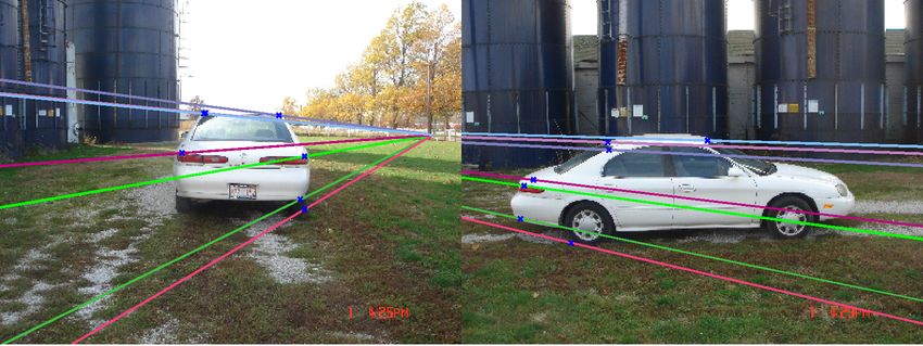
P1(cx,cy,cz) P2(cx,cy,cz) link to recognizing objects in 2D images is established by
P1 P2 projecting the 3D parts to a number of distinct viewpoints,
(cx,cy,cz) “observed” by viewpoint dependent mixture components, in
(x,y,z) analogy to DPM-VOC+VP. Since all components observe
P1(x,y,z) = (u1,v1) P2(x,y,z) = (u2,v2)
the parts through a fixed, deterministic mapping (the pro-
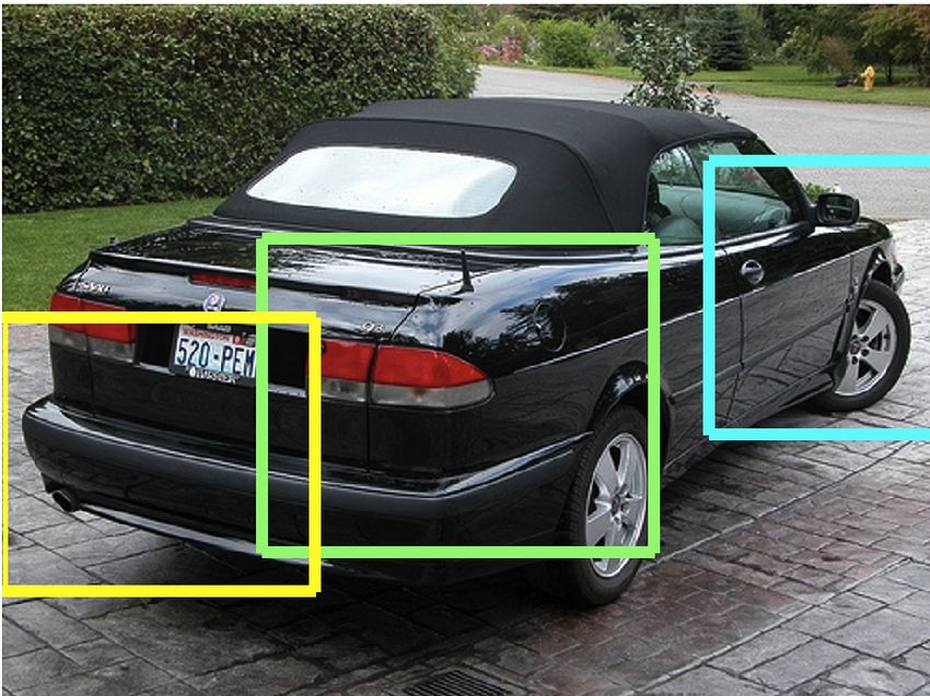
Figure 2. 3D part parametrization for an example 3D CAD model jections), their appearances as well as their deformations
(center). Corresponding projected part positions in 2 different are linked and kept consistent across viewpoints by design.
views, overlaid non-photorealistic renderings [28] (left, right).
3D Parametrization. Given a 3D CAD model of the ob-
viewpoint annotation. During training, we then find the op- ject class of interest, we parametrize a part as an axis-
timal part placements for the single component matching aligned, 3D bounding cube of a fixed size per object class,
the annotation for the training examples (which speeds up pj = (xj , yj , zj ), positioned relative to the object center (its
training). For training examples where a viewpoint is not root, see Fig. 2), in analogy to positioning parts relative to
annotated we proceed with standard DPM training, maxi- the root filter in 2D for DPM-Hinge. Further, we assume a
mizing over components as well. At test time we output the fixed anchor position for each part pj , from which pj will
estimated mixture component as a viewpoint estimate. typically move away during training, in the course of maxi-
Since the component-viewpoint association alone does mizing latent part positions h.
not yet encourage the model to estimate the correct view-
point (because Eq. (3) does not penalize constraints that Model structure. The DPM-3D-Constraints consists of a
yield the correct BB location but a wrong viewpoint esti- number of viewpoint dependent mixture components, and
mate), we exploit that our objective function is defined for is thus structurally equivalent to the DPM-VOC+VP. Each
general loss functions. We add a 0/1 loss term for the view- component observes the 3D space from a specific viewpoint
point variables, in the following convex combination c, defined by a projective mapping P c . In full analogy to the
DPM-VOC+VP, for each part pj , each component observes
∆VOC+VP (y, ȳ) = (1 − α)∆VOC (y, ȳ) + α [y v 6= ȳ v ] . (5) i) part appearance as well as ii) part displacement. Here,
Note that any setting α 6= 0 is likely to decrease 2D BB both are uniquely determined by the projection P c (pj ). For
localization performance. Nevertheless we set α = 0.5 in i), we follow [28] to generate a non-photorealistic, gradient-
all experiments and show empirically that the decrease in based rendering of the 3D CAD model, and extract a HOG
detection performance is small, while we gain an additional filter for the part pj directly from that rendering. For ii), we
viewpoint estimate. Note also, that the constraint set from measure the displacement between the projected root and
Eq. (3) now include those cases where the BB location is the projected part position. Part’s displacement distribution
estimated correctly but the estimated mixture component (in is defined in the image plane and it is independent across
h) does not coincide with the true viewpoint. components. As a short-hand notation, we include the pro-
A less powerful but straight-forward extension to DPM- jection into the feature function Ψ(Ii , yi , h, P c ).
Hinge is to use the viewpoint annotations as an initialization
Learning. Switching to the 3D parametrization requires
for the mixture components, which we refer to in our exper-
to optimize latent part placements h over object instances
iments as DPM-Hinge-VP.
(possibly observed from multiple viewpoints simultane-
ously) rather than over individual images. Formally, we
introduce an object ID variable y o to be included in the an-
3.2. Introducing 3D parts (DPM-3D-Constraints)
notation y. For a training instance y o , we let S(y o ) := {i :
The second extension constitutes a fundamental change yio = y o } and compute
to the model, namely, a parametrization of latent part po- X D E
v
sitions in 3D object space rather than in 2D image coordi- h∗ = argmax β, Ψ(Ii , yi , h, P yi ) . (6)
nates. It is based on the intuition that parts should really h
i∈S(y o )
live in 3D object space rather than in the 2D image plane,
and that a part is defined as a certain partial volume of a 3D This problem can be solved analogously to its 2D coun-
object rather than as a 2D BB. terpart DPM-VOC+VP: assuming a fixed placement of the
We achieve this by basing our training procedure on a object root (now in 3D), we search for the best place-
set of 3D CAD models of the object class of interest that ment h of each of the parts also in 3D. The score of the
we use in addition to real training images. Being formed placement then depends simultaneously on all observing
from triangular surface meshes, 3D CAD models provide viewpoint-dependent components, since changing h poten-
3D geometric descriptions of object class instances, lend- tially changes all projections. The computation of the maxi-
ing themselves to 3D volumetric part parametrizations. The mum is still a linear operation in the number of possible 3D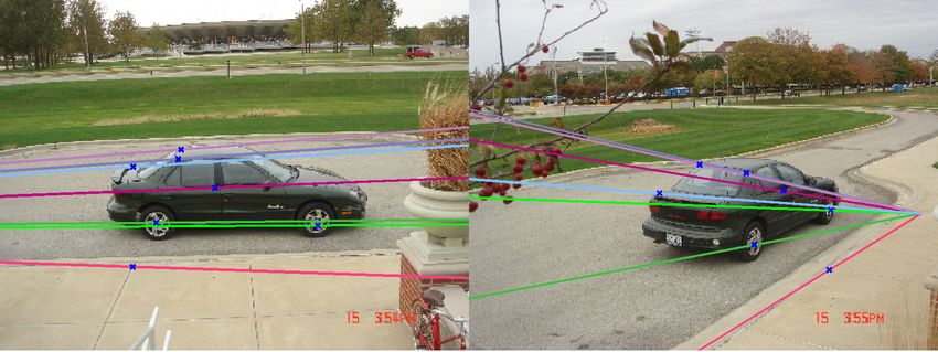
AP         aero   bird   bicyc   boat   bottle   bus    car    cat    cow    table    dog    horse   mbike   person   plant   sheep   sofa   train   tv     chair   AVG
 DPM-Hinge      30.4   1.8    61.1    13.1   30.4     50.0   63.6   9.4    30.3   17.2     1.7    56.5    48.3    42.1     6.9     16.5    26.8   43.9    37.6   18.5    30.3
  DPM-VOC       31.1   2.7    61.3    14.4   29.8     51.0   65.7   12.4   32.0   19.1     2.0    58.6    48.8    42.6     7.7     20.5    27.5   43.7    38.7   18.7    31.4
 Vedaldi [32]   37.6   15.3   47.8    15.3   21.9     50.7   50.6   30.0   33.0   22.5     21.5   51.2    45.5    23.3     12.4    23.9    28.5   45.3    48.5   17.3    32.1

Table 1. 2D bounding box localization performance (in AP) on Pascal VOC 2007 [9], comparing DPM-Hinge, DPM-VOC, and [32]. Note
that [32] uses a kernel combination approach that makes use of multiple complementary image features.
placements, and we use the same optimization algorithm                                    task on all 20 classes of the challenging Pascal VOC 2007
as before: alternate between a) updating β and b) updat-                                  data set [9]. Second, we give results on 9 classes of the 3D
ing h and searching for violating constraints. Note that                                  Object Classes data set [27], which has been proposed as a
the DPM-3D-Constraints introduces additional constraints                                  testbed for multi-view recognition, and is considered chal-
to the training examples and thereby lowers the number of                                 lenging because of its high variability in viewpoints (objects
free parameters of the model. We attribute performance dif-                               are imaged from 3 different distances, 3 elevations, and 8
ferences to DPM-VOC+VP to this fact.                                                      azimuth angles). In all experiments, we use images from
                                                                                          the respective data sets for training (sometimes in addition
Blending with real images. Training instances for which                                   to our synthetic data), following the protocols established
there is only a single 2D image available (e.g., Pascal VOC                               as part of the data sets [9, 27].
data) can of course be used during training. Since there are
no other examples that constrain their 3D part placements,                                2D Bounding box localization. Tab. 1 gives results for
they are treated as before in (2). Using real and synthetic                               2D BB localization according to the Pascal criterion, re-
images for training is called mixed in the experiments.                                   porting per-class average precision (AP). It compares our
                                                                                          DPM-VOC (row 2) to the DPM-Hinge [11] (row 1) and
Initialization. In contrast to prior work relying on hand-
                                                                                          to the more recent approach [32] (row 3), both of which
labeled semantic parts [28, 36], we initialize parts in the ex-
                                                                                          are considered state-of-the-art on this data set. We first ob-
act data-driven fashion of the DPM, only in 3D: we choose
                                                                                          serve that DPM-VOC outperforms DPM-Hinge on 18 of
greedily k non-overlapping parts with maximal combined
                                                                                          20 classes, and [32] on 8 classes. While the relative per-
appearance score (across views).
                                                                                          formance difference of 1.1% on average (31.4% AP vs.
Self-occlusion reasoning. Training from CAD data al-                                      30.3% AP) to DPM-Hinge is moderate in terms of numbers,
lows to implement part-level self-occlusion reasoning ef-                                 it is consistent, and speaks in favor of our structured loss
fortlessly, using a depth buffer. In each view, we thus limit                             over the standard hinge-loss. In comparison to [32] (32.1%
the number of parts to the l ones with largest visible area.                              AP), DPM-VOC loses only 0.7% while the DPM-Hinge has
                                                                                          1.8% lower AP. We note that [32] exploits a variety of dif-
4. Experiments                                                                            ferent features for performance, while the DPM models rely
                                                                                          on HOG features, only.
   In this section, we carefully evaluate the performance of                                  Tab. 2 gives results for 9 3D Object Classes [27], com-
our approach, analyzing the impact of successively adding                                 paring DPM-Hinge (col. 1), DPM-VOC+VP (col. 3), and
3D geometric information as we proceed. We first evalu-                                   DPM-Hinge-VP (col. 2), where we initialize and fix each
ate the 2D BB localization of our structured loss formula-                                component of the DPM-Hinge with training data from just
tion, trained using only ∆VOC (DPM-VOC, Sect. 2.2). We                                    a single viewpoint, identical to DPM-VOC+VP. We observe
then add viewpoint information by optimizing for ∆VOC+VP                                  a clear performance ordering, improving from DPM-Hinge
(DPM-VOC+VP, Sect. 3.1), enabling simultaneous 2D BB                                      over DPM-Hinge-VP to DPM-VOC+VP, which wins for 5
localization and viewpoint estimation. Next, we add syn-                                  of 9 classes. While the average improvement is not as pro-
thetic training images (Sect. 3.2), improving localization                                nounced (ranging from 88.0% over 88.4% to 88.7% AP), it
and viewpoint estimation accuracy. Finally, we switch to                                  confirms the benefit of structured vs. hinge-loss.
the 3D parameterization of latent part positions during train-
ing (DPM-3D-Constraints, Sect. 3.2), and leverage the re-                                 Viewpoint estimation. Tab. 2 also gives results for view-
sulting consistency of parts across viewpoints in an ultra-                               point estimation, phrased as a classification problem, distin-
wide baseline matching task. Where applicable, we com-                                    guishing among 8 distinct azimuth angle classes. For DPM-
pare to both DPM-Hinge and results of related work.                                       Hinge, we predict the most likely viewpoint by collecting
                                                                                          votes from training example annotations for each compo-
4.1. Structured learning
                                                                                          nent. For DPM-Hinge-VP and DPM-VOC+VP, we use
   We commence by comparing the performance of DPM-                                       the (latent) viewpoint prediction. In line with previous
VOC to the original DPM (DPM-Hinge), using the imple-                                     work [27, 21], we report the mean precision in pose esti-
mentation of [11]. For this purpose, we evaluate on two                                   mation (MPPE), equivalent to the average over the diagonal
diverse data sets. First, we report results for the detection                             of the 8 (viewpoint) class confusion matrix. Clearly, the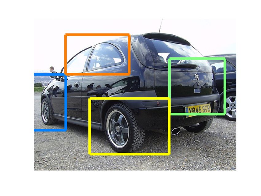
AP / MPPE   DPM-Hinge     DPM-Hinge-VP DPM-VOC+VP            Second, we observe that DPM-VOC improves significantly
          iron     94.7 / 56.0   93.3 / 86.3   96.0 / 89.7          (from 24.7% to 34.5% AP) over DPM-Hinge for synthetic
          shoe     95.2 / 59.7   97.9 / 71.0   96.9 / 89.8          on cars, highlighting the importance of structured training.
        stapler    82.8 / 61.4   84.4 / 62.8   83.7 / 81.2          Third, we see that mixed consistently outperforms real for
        mouse      77.1 / 38.6   73.1 / 62.2   72.7 / 76.3
                                                                    DPM-VOC, obtaining state-of-the-art performance for both
       cellphone   60.4 / 54.6   62.9 / 65.4   62.4 / 83.0
         head      87.6 / 46.7   89.6 / 89.3   89.9 / 89.6          cars (66.0% AP) and bicycles (61.6% AP).
        toaster    97.4 / 45.0   96.0 / 50.0   97.8 / 79.7              Tab. 3 (right) gives results for 3D Object Classes, again
           car     99.2 / 67.1   99.6 / 92.5   99.8 / 97.5          training from real, synthetic, and mixed data, sorting results
        bicycle    97.9 / 73.1   98.6 / 93.0   98.8 / 97.5          of recent prior work into the appropriate rows. In line with
         AVG       88.0 / 55.8   88.4 / 74.7   88.7 / 87.1          our findings on Pascal, we observe superior performance of
Table 2. 2D bounding box localization (in AP) and viewpoint esti-   DPM-VOC+VP over DPM-Hinge, as well as prior work.
mation (in MPPE [21]) results on 9 3D Object classes [27].          Surprisingly, synthetic (98.6% AP) performs on cars almost
                                                                    on par with the best reported prior result [13] (99.2%).
average MPPE of 87.1% of DPM-VOC+VP outperforms                     Mixed improves upon their result to 99.9% AP. On bicy-
DPM-Hinge-VP (74.7%) and DPM-Hinge (55.8%). It also                 cles, the appearance differences between synthetic and real
outperforms published results of prior work [21] (79.2%)            data are more pronounced, leading to a performance drop
and [14] (74.0%) by a large margin of 7.9%. Initializing            from 98.8% to 78.1% AP, which is still superior to DPM-
with per-viewpoint data already helps (59.8% vs. 74.7%),            Hinge synthetic (72.2% AP) and the runner-up prior result
but we achieve a further boost in performance by applying           of [20] (69.8% AP), which uses mixed training data.
a structured rather than hinge-loss (from 74.7% to 87.14%).             In Fig. 3, we give a more detailed analysis of training
As a side result we find that the standard DPM benefits from        DPM-Hinge and DPM-VOC from either real or mixed data
initializing the components to different viewpoints. We ver-        for 3D Object Classes [27] (left) and Pascal 2007 [9] (mid-
ified that fixing the components does not degrade perfor-           dle, right) cars. In the precision-recall plot in Fig. 3 (mid-
mance, this is a stable local minima. This makes evident            dle), DPM-VOC (blue, magenta) clearly outperforms DPM-
that different viewpoints should be modeled with different          Hinge (red, green) in the high-precision region of the plot
mixture components. A nice side effect is that training is          (between 0.9 and 1.0) for both real and mixed, confirming
faster when fixing mixture components.                              the benefit of structured max-margin training. From the re-
Summary. We conclude that structured learning results in            call over BB overlap at 90% precision plot in Fig. 3 (right),
a modest, but consistent performance improvement for 2D             we further conclude that for DPM-Hinge, mixed (green)
BB localization. It significantly improves viewpoint esti-          largely improves localization over real (red). For DPM-
mation over DPM-Hinge as well as prior work.                        VOC, real (blue) is already on par with mixed (magenta).

4.2. Synthetic training data                                        Viewpoint estimation. In Tab. 3 (right), we observe dif-
                                                                    ferent behaviors of DPM-Hinge and DPM-VOC+VP for
   In the following, we examine the impact of enriching             viewpoint estimation, when considering the relative per-
the appearance models of parts and whole objects with syn-          formance of real, synthetic, and mixed. While for DPM-
thetic training data. For that purpose, we follow [28] to gen-      VOC+VP, real is superior to synthetic for both cars and bi-
erate non-photorealistic, gradient-based renderings of 3D           cycles (97.5% vs. 92.9% and 97.5% vs. 86.4%), the DPM-
CAD models, and compute HOG features directly on those              Hinge benefits largely from synthetic training data for view-
renderings. We use 41 cars and 43 bicycle models1 as we             point classification (improving from 67.1% to 78.3% and
have CAD data from these two classes only.                          from 73.1% to 77.5%). In this case, the difference in fea-
                                                                    ture statistics can apparently be outbalanced by the more
2D bounding box localization. We again consider Pascal
                                                                    accurate viewpoints provided by synthetic.
VOC 2007 and 3D Object Classes, but restrict ourselves to
                                                                       For both, DPM-Hinge and DPM-VOC+VP, mixed beats
the two object classes most often tested by prior work on
                                                                    either of real and synthetic, and switching from DPM-Hinge
multi-view recognition [20, 28, 25, 13, 36], namely, cars
                                                                    to DPM-VOC+VP improves performance by 11.6% for cars
and bicycles. Tab. 3 (left) gives results for Pascal cars and
                                                                    and 25.8% for bicycles, beating runner-up prior results by
bicycles, comparing DPM-Hinge (col. 2) and DPM-VOC
                                                                    11.8% and 18.1%, respectively.
(col. 3) with the recent results of [13] (col. 1) as a refer-
ence. We compare 3 different training sets, real, synthetic,
                                                                    Summary. We conclude that adding synthetic training
and mixed. First, we observe that synthetic performs con-
                                                                    data in fact improves the performance of both 2D BB local-
siderably worse than real in all cases, which is understand-
                                                                    ization and viewpoint estimation. Using mixed data yields
able due to their apparent differences in feature statistics.
                                                                    state-of-the-art results for cars and bicycles on both Pascal
  1 www.doschdesign.com,   www.sketchup.google.com/3dwarehouse/     VOC 2007 and 3D Object classes.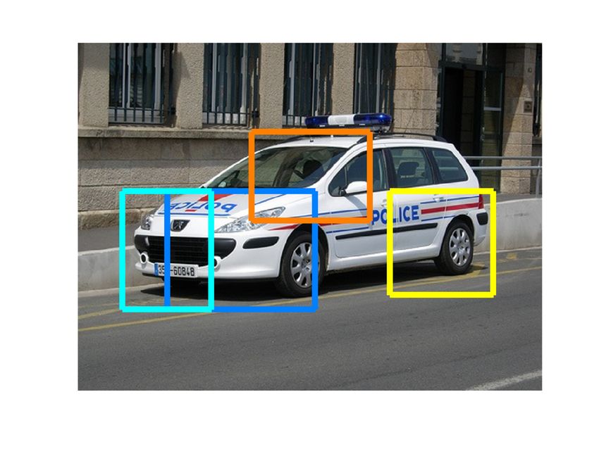
Pascal 2007 [9] 3D Object Classes [27]
AP / MPPE Glasner [13] DPM-Hinge DPM-VOC DPM-3D-Const. Liebelt [20] Zia [36] Payet [25] Glasner [13] DPM-Hinge DPM-VOC+VP DPM-3D-Const.
real 32.0 63.6 65.7 - - - - / 86.1 99.2 / 85.3 99.2 / 67.1 99.8 / 97.5 -
cars
synthetic - 24.7 34.5 24.9 - 90.4 / 84.0 - - 92.1 / 78.3 98.6 / 92.9 94.3 / 84.9
mixed - 65.6 66.0 63.1 76.7 / 70 - - - 99.6 / 86.3 99.9 / 97.9 99.7 / 96.3
real - 61.1 61.3 - 98.8 / 97.5
bicycle
- - - / 80.8 - 97.9 / 73.1 -
synthetic - 22.6 25.2 20.7 - - - - 72.2 / 77.5 78.1 / 86.4 72.4 / 82.0
mixed - 60.7 61.6 56.8 69.8 / 75.5 - - - 97.3 / 73.1 97.6 / 98.9 95.0 / 96.4
Table 3. 2D bounding box localization (in AP) on Pascal VOC 2007 [9] (left) and 3D Object Classes [27] (right). Viewpoint estimation (in
MPPE [21]) on 3D Object Classes (right). Top three rows: object class car, bottom three rows: object class bicycle.
1 1 0.7
DPM−VOC, real data
0.9 DPM Hinge, real data
0.6 DPM−VOC, mixed data
0.95 DPM−Hinge, mixed data
0.8
DPM−3D−Constraints, mixed data
0.7 0.5
0.9
0.6
0.4
Recall
recall
recall
0.85 0.5
0.3
0.4
0.8
0.3 0.2
DPM−Hinge, real data (AP = 99.2) DPM−Hinge, real data (AP = 63.6)
DPM−Hinge, mixed data (AP = 99.6) DPM−Hinge, mixed data (AP = 64.9)
0.2
0.75 DPM−VOC, real data (AP = 99.8) DPM−VOC, real data (AP = 65.7)
0.1
DPM−VOC, mixed data (AP = 99.9) DPM−VOC, mixed data (AP = 66.0)
0.1
DPM−3D−Constraints, mixed data (AP = 99.7) DPM−3D−Constraints, mixed data (AP = 63.1)
0.7 0 0
0 0.05 0.1 0.15 0.2 0.25 0.3 0 0.2 0.4 0.6 0.8 1 50 60 70 80 90 100
1 − precision 1 − precision bounding box overlap
Figure 3. Detailed comparison of real and mixed training data. Left: Precision-recall on 3D Object Classes [27] cars (zoomed). Middle:
Precision-recall on Pascal VOC 2007 [9] cars. Right: Recall over bounding box overlap at 90% precision on Pascal 2007 cars.
4.3. 3D deformable parts adapt the experimental setting proposed by [36], and use
corresponding part positions on two views of the same ob-
We finally present results for the DPM-3D-Constraints,
ject as inputs to a structure-from-motion (SfM) algorithm.
constraining latent part positions to be consistent across
We then measure the Sampson error [17] of the resulting
viewpoints. We first verify that this added geometric ex-
fundamental matrix(see Fig. 4), using ground truth corre-
pressiveness comes at little cost w.r.t. 2D BB localization
spondences. We use the same subset of 3D Object Classes
and viewpoint estimation, and then move on to the more
cars as [36], yielding 134 image pairs, each depicting the
challenging task of ultra-wide baseline matching, which is
same object from different views, against static background.
only enabled by enforcing across-viewpoint constraints.
Tab. 4 gives the results (percentage of estimated fundamen-
2D bounding box localization. In Tab. 3 (left, last col.), tal matrices with a Sampson error < 20 pixels), compar-
we observe a noticeable performance drop from DPM-VOC ing a simple baseline using SIFT point matches (col. 1) to
to DPM-3D-Constraints for both Pascal cars and bicycles the results by [36] (col. 2), and the DPM-3D-Constraints
for synthetic (from 34.5% to 24.9% and 25.2% to 20.7% using 12 (col. 3) and 20 parts (col. 4), respectively, for
AP, respectively). Interestingly, this drop is almost en- varying angular baselines between views. As expected, the
tirely compensated by mixed, leaving us with remarkable SIFT baseline fails for views with larger baselines than 45◦ ,
63.1% AP for cars and 56.8% AP for bicycles, close to since the appearance of point features changes too much
the state-of-the-art results (DPM-Hinge). Tab. 3 (right, last to provide matches. On the other hand, we observe com-
col.) confirms this result for 3D Object Classes. DPM-3D- petitive performance of our 20 part DPM-3D-Constraints
Constraints obtains 0.2% lower AP for cars and 2.6% lower compared to [36] for baselines between 45◦ and 135◦ , and
AP for bicycles, maintaining performance on par with the a significant improvement of 29.4% for the widest baseline
state-of-the-art. (180◦ ), which we attribute to the ability of our DPM-3D-
Constraints to robustly distinguish between opposite view
Viewpoint estimation. The switch from DPM-VOC+VP points, while [36] reports confusion for those cases.
to DPM-3D-Constraints results in performance drop, which Azimuth SIFT Zia [36] DPM-3D-Const. 12 DPM-3D-Const. 20
we attribute to the reduced number of parameters due to the 45 ◦ 2.0% 55.0% 49.1% 54.7%
additional 3D constraints. Still, this performance drop is 90 ◦ 0.0% 60.0% 42.9% 51.4%
rather small. In particular for mixed (we lose only 1.3% 135 ◦ 0.0% 52.0% 55.2% 51.7%
MPPE for cars and 2.5% for bicycles). 180 ◦ 0.0% 41.0% 52.9% 70.6%
AVG 0.5% 52.0% 50.0% 57.1%
Ultra-wide baseline matching. In this experiment, we
Table 4. Ultra-wide baseline matching performance, measured as
quantify the ability of the DPM-3D-Constraints to hypothe- fraction of correctly estimated fundamental matrices. Results for
size part positions that are consistent across viewpoints. We DPM-3D-Const. with 12 and 20 parts versus state-of-the-art.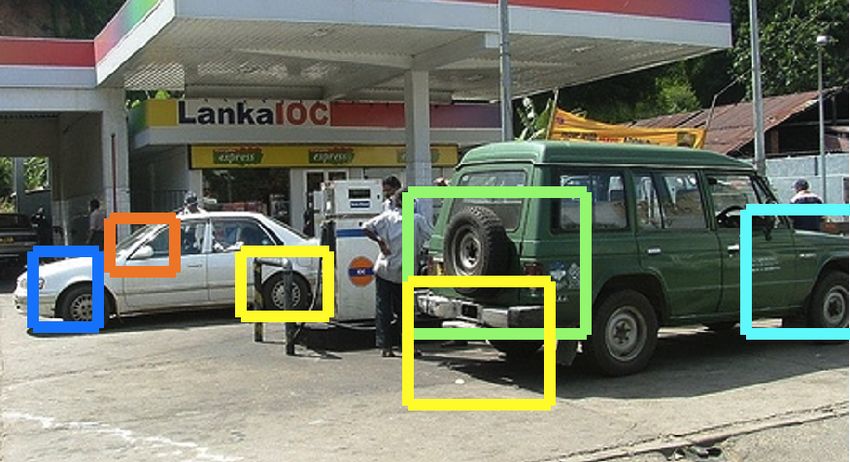
Figure 4. Example ultra-wide baseline matching [36] output. Estimated epipoles and epipolar lines (colors correspond) for image pairs.

Summary. Our results confirm that the DPM-3D-                               [13] D. Glasner, M. Galun, S. Alpert, R. Basri, and G. Shakhnarovich.
Constraints provides robust estimates of part positions that                     Viewpoint-aware object detection and pose estimation. In ICCV,
                                                                                 2011. 2, 6, 7
are consistent across viewpoints, and hence lend themselves                 [14] C. Gu and X. Ren. Discriminative mixture-of-templates for view-
to 3D geometric reasoning. At the same time, the DPM-3D-                         point classification. In ECCV, 2010. 2, 6
Constraints maintains performance on par with state-of-the-                 [15] A. Gupta, A. A. Efros, and M. Hebert. Blocks world revisited: Image
art for both 2D BB localization and viewpoint estimation.                        understanding using qualitative geometry and mechanics. In ECCV,
                                                                                 2010. 1
                                                                            [16] A. Gupta, S. Satkin, A. A. Efros, and M. Hebert. From 3D scene
5. Conclusions                                                                   geometry to human workspace. In CVPR, 2011. 1
   We have shown how to teach 3D geometry to DPMs,                          [17] R. I. Hartley and A. Zisserman. Multiple View Geometry in Computer
aiming to narrow the representational gap between state-of-                      Vision. Cambridge University Press, 2004. 7
                                                                            [18] D. Hoiem, A. Efros, and M. Hebert. Putting objects in perspective.
the-art object class detection and scene-level, 3D geometric                     IJCV, 2008. 1
reasoning. By adding geometric information on three differ-                 [19] B. Leibe, A. Leonardis, and B. Schiele. An implicit shape model
ent levels, we improved performance over the original DPM                        for combined object categorization and segmentation. In Toward
and prior work. We achieved improvements for 2D bound-                           Category-Level Object Recognition, 2006. 1, 2
                                                                            [20] J. Liebelt and C. Schmid. Multi-view object class detection with a
ing box localization, viewpoint estimation, and ultra-wide                       3D geometric model. In CVPR, 2010. 2, 6, 7
baseline matching, confirming the ability of our model to                   [21] R. J. Lopez-Sastre, T. Tuytelaars, and S. Savarese. Deformable part
deliver more expressive hypotheses w.r.t. 3D geometry than                       models revisited: A performance evaluation for object category pose
prior work, while maintaining or even increasing state-of-                       estimation. In ICCV-WS CORP, 2011. 5, 6, 7
                                                                            [22] D. Lowe. Three-dimensional object recognition from single two-
the-art performance in 2D bounding box localization .                            dimensional images. Artificial Intelligence, 1987. 1, 2
                                                                            [23] D. Marr and H. Nishihara. Representation and recognition of the
Acknowledgements This work has been supported by the                             spatial organization of three-dimensional shapes. Proc. Roy. Soc.
Max Planck Center for Visual Computing and Communica-                            London B, 200(1140):269–194, 1978. 1, 2
tion. We thank M. Zeeshan Zia for his help in conducting                    [24] M. Ozuysal, V. Lepetit, and P. Fua. Pose estimation for category
wide baseline matching experiments.                                              specific multiview object localization. In CVPR, 2009. 2
                                                                            [25] N. Payet and S. Todorovic. From contours to 3d object detection and
References                                                                       pose estimation. In ICCV, 2011. 6, 7
                                                                            [26] A. Pentland. Perceptual organization and the representation of natu-
 [1] M. Arie-Nachimson and R. Basri. Constructing implicit 3D shape              ral form. Artificial Intelligence, 28, 1986. 1, 2
     models for pose estimation. In ICCV, 2009. 2                           [27] S. Savarese and L. Fei-Fei. 3D generic object categorization, local-
 [2] S. Y. Bao and S. Savarese. Semantic structure from motion. In CVPR,         ization and pose estimation. In ICCV, 2007. 2, 3, 5, 6, 7
     2011. 1, 2                                                             [28] M. Stark, M. Goesele, and B. Schiele. Back to the future: Learning
 [3] V. Blanz and T. Vetter. Face recognition based on fitting a 3d mor-         shape models from 3d cad data. In BMVC, 2010. 2, 4, 5, 6
     phable model. PAMI, 2003. 2                                            [29] H. Su, M. Sun, L. Fei-Fei, and S. Savarese. Learning a dense multi-
 [4] M. Blaschko and C. Lampert. Learning to localize objects with struc-        view representation for detection, viewpoint classification and syn-
     tured output regression. In ECCV, 2008. 3                                   thesis of object categories. In ICCV, 2009. 2
 [5] R. Brooks. Symbolic reasoning among 3-d models and 2-d images.         [30] M. Sun, B. Xu, G. Bradski, and S. Savarese. Depth-encoded hough
     Artificial Intelligence, 17:285–348, 1981. 1, 2                             voting for joint object detection and shape recovery. In ECCV’10. 2
 [6] N. Dalal and B. Triggs. Histograms of oriented gradients for human     [31] A. Thomas, V. Ferrari, B. Leibe, T. Tuytelaars, B. Schiele, and
     detection. In CVPR, 2005. 3                                                 L. Van Gool. Towards multi-view object class detection. In CVPR,
 [7] A. Ess, B. Leibe, K. Schindler, and L. V. Gool. Robust multi-person         2006. 2
     tracking from a mobile platform. PAMI, 2009. 1                         [32] A. Vedaldi, V. Gulshan, M. Varma, and A. Zisserman. Multiple ker-
 [8] M. Everingham, L. Gool, C. K. Williams, J. Winn, and A. Zisserman.          nels for object detection. In ICCV, 2009. 5
     The pascal visual object classes (voc) challenge. IJCV, 2010. 1        [33] H. Wang, S. Gould, and D. Koller. Discriminative learning with la-
 [9] M. Everingham, L. Van Gool, C. K. I. Williams, J. Winn, and A. Zis-         tent variables for cluttered indoor scene understanding. In ECCV’10.
     serman. The PASCAL VOC 2007 Results. 2, 5, 6, 7                             1
[10] P. F. Felzenszwalb, R. Girshick, D. McAllester, and D. Ramanan.        [34] C. Wojek, S. Roth, K. Schindler, and B. Schiele. Monocular 3d scene
     Object detection with discriminatively trained part based models.           modeling and inference: Understanding multi-object traffic scenes.
     PAMI, 2009. 1, 2, 3                                                         In ECCV, 2010. 1
[11] P. F. Felzenszwalb, R. B. Girshick, and D. McAllester. Dis-            [35] P. Yan, S. Khan, and M. Shah. 3D model based object class detection
     criminatively trained deformable part models, release 4.                    in an arbitrary view. In ICCV, 2007. 2
     http://www.cs.brown.edu/ pff/latent-release4/. 5                       [36] Z. Zia, M. Stark, K. Schindler, and B. Schiele. Revisiting 3d geomet-
                                                                                 ric models for accurate object shape and pose. In 3dRR-11, 2011. 2,
[12] R. Fergus, P. Perona, and A. Zisserman. Object class recognition by
                                                                                 5, 6, 7, 8
     unsupervised scale-invariant learning. In CVPR, 2003. 1, 2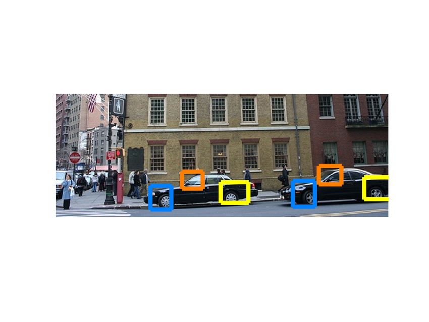
You can also read