THE GOOGLE EARTH ENGINE DIGITISATION TOOL (GEEDIT) AND THE MARGIN CHANGE QUANTIFICATION TOOL (MAQIT) - SIMPLE TOOLS FOR THE RAPID MAPPING AND ...
←
→
Page content transcription
If your browser does not render page correctly, please read the page content below
Earth Surf. Dynam., 6, 551–561, 2018
https://doi.org/10.5194/esurf-6-551-2018
© Author(s) 2018. This work is distributed under
the Creative Commons Attribution 4.0 License.

       The Google Earth Engine Digitisation Tool (GEEDiT) and
       the Margin change Quantification Tool (MaQiT) – simple
           tools for the rapid mapping and quantification of
                    changing Earth surface margins
                                                        James M. Lea
           Department of Geography annd Planning, School of Environmental Sciences, University of Liverpool,
                                              Liverpool, L69 7ZT, UK
                                 Correspondence: James M. Lea (j.lea@liverpool.ac.uk)

                                 Received: 11 March 2018 – Discussion started: 22 March 2018
                             Revised: 4 June 2018 – Accepted: 4 July 2018 – Published: 13 July 2018

      Abstract. Changes in margins derived from satellite imagery are quantitative indicators of the environmental
      processes and drivers acting on the Earth’s surface, for example retreating ice margins or coastal changes with
      rising sea level. However, the large-scale rapid visualisation and analysis of the satellite record is often imprac-
      tical due to factors such as computer processing power, software availability, internet connection speed and/or
      user expertise in remote sensing. Here are presented three new, freely accessible tools that together can be used
      to process, visualise and review data from the full Landsat 4–8 and Sentinel 1–2 satellite records in seconds, en-
      abling efficient mapping (through manual digitisation) and automated quantification of margin changes. These
      tools are highly accessible for users from a range of remote-sensing expertise (from academics to high school
      students), with minimal computational, licensing and knowledge-based barriers to access. The Google Earth
      Engine Digitisation Tool (GEEDiT) allows users to define a point anywhere on the planet and filter data from
      each satellite for user-defined time frames, maximum acceptable cloud cover extent, and options of predefined
      or custom image band combinations via a simple graphical user interface (GUI). GEEDiT allows georeferenced
      vectors to be easily and rapidly mapped from each image, with image metadata and user notes automatically
      appended to each vector, which can then be exported for subsequent analysis. The GEEDiT Reviewer tool al-
      lows users to quality control their own/others’ data and also filter existing datasets based on the spatial/temporal
      requirements for their particular research question. The Margin change Quantification Tool (MaQiT) is com-
      plementary to GEEDiT and GEEDiT Reviewer, allowing the rapid quantification of these margin changes by
      utilising two well-established methods that have previously been used to measure glacier margin change and
      two new methods via a similarly simple GUI. A case study of the lake-terminating glacier Breiðamerkurjökull,
      Iceland, is used to demonstrate the complementary functionality of GEEDiT, GEEDiT Reviewer and MaQiT,
      though it should be noted that MaQiT is also suitable for the (re-)analysis of existing datasets not generated by
      GEEDiT. MaQiT has been developed with the original aim of quantifying tidewater glacier terminus change,
      though the methods included within the tool have potential for wide applications in multiple areas of Earth sur-
      face science (e.g. coastal and vegetation extent change). It is hoped that these tools will allow a wide range of
      researchers and students across the geosciences to efficiently map, analyse and access volumes of data that would
      have previously proven prohibitive.

Published by Copernicus Publications on behalf of the European Geosciences Union.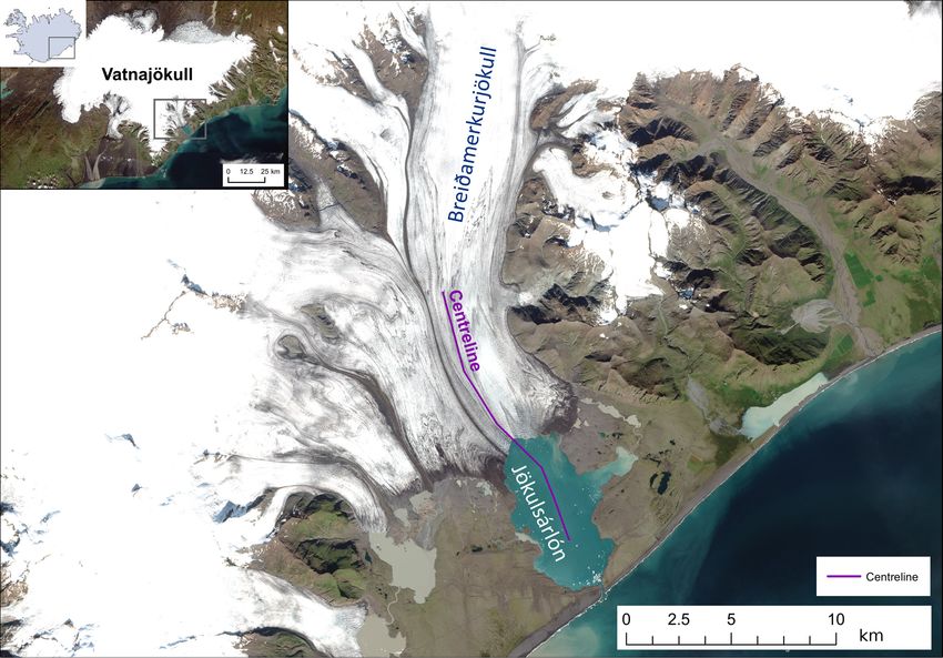
552                                                James M. Lea: Rapid mapping and quantification of Earth surface margins

1   Introduction                                                    and images. The second is the GEEDiT Reviewer tool that
                                                                    allows data previously generated by GEEDiT to be qual-
Satellite data provide an invaluable record of spatial and          ity controlled and filtered. The third is the Margin change
temporal change on the Earth’s surface. However, the vol-           Quantification Tool (MaQiT) that allows the rapid quantifi-
ume and scale of data available for analysis (coupled with          cation of these digitised margin changes, utilising two ex-
computational, software licensing, data storage, internet con-      isting methods (Lea et al., 2014) and two new methods that
nectivity and knowledge-based barriers to entry) mean that          have commonly been used in the quantification of tidewa-
users may require a significant amount of time to go from           ter glacier margin change. Although initially developed for
downloading an image to finalising its analysis. This can be        glaciological applications, each of these quantification meth-
exemplified in the study of tidewater glacier calving mar-          ods are likely to have applications in the quantification of
gins where a large volume of remote-sensing imagery ex-             margin change in other areas of Earth surface sciences such
ists, though spatially large-scale studies are often required to    as coastal change, lake level evolution, and vegetation and
focus on a number of census time frames (e.g. Cook et al.,          urban extent change, amongst others.
2005; Moon and Joughin, 2008; Carr et al., 2017; Bunce et
al., 2018), while detailed studies often focus on a relatively
small number of sites (e.g. Bevan et al., 2012; Motyka et al.,      2   Google Earth Engine Digitisation Tool (GEEDiT)
2017).                                                                  and GEEDiT Reviewer
   The availability of satellite imagery via application pro-
gramming interfaces (APIs) and increasingly via platforms           GEEDiT and GEEDiT Reviewer are written in JavaScript
such as Google Earth Engine (Gorelick et al., 2017), Sen-           within Google Earth Engine’s (GEE) API (Gorelick et al.,
tinel Hub’s Earth Observation Explorer (Sinergise, 2018) and        2017). GEEDiT is designed to allow satellite imagery from
Planet (Planet Labs Inc., 2018) means that these data are be-       Landsat 4–8 and Sentinel 1–2 to be visualised rapidly within
coming increasingly accessible. However, the ability of users       a standard web browser, also allowing the digitisation and
to access these data at such a large scale is currently lim-        export of polyline and/or polygon vector data in GeoJ-
ited by the need for either knowledge of coding and/or for          SON (Georeferenced JavaScript Object Notation format) or
downloading, storage and processing of substantial volumes          KML/KMZ (Keyhole Markup Language/Keyhole Markup
of data. Even where users are comfortable with such require-        Zipped format compatible with Google Earth) formats. GEE
ments, images may still prove time-consuming to effectively         does not currently support the export of data in shapefile for-
visualise and finally analyse, thus taking further time. This       mat, though a tool is included within MaQiT to both merge
can severely limit the scale of analysis that it is practical for   and convert GeoJSON files to a single shapefile (see Sect. 3).
researchers to undertake.                                           This means that data digitised during multiple GEEDiT
   The identification of temporally evolving margins digi-          sessions can be merged and/or converted for use either in
tised from this imagery is frequently used across Earth sur-        MaQiT or a traditional geographic information system (GIS)
face sciences to provide key temporal and/or spatial insight        platform.
into the system of interest (e.g. Kuenzer et al., 2014; Roelf-         The GEEDiT Reviewer tool is separate to GEEDiT, allow-
sema et al., 2013; Fitzpatrick et al., 2014; Lynch et al., 2016).   ing users to review existing datasets generated by GEEDiT.
Although different geoscientific problems will have differ-         It can be used to both quality control their own and others’
ent temporal and spatial data coverage requirements, a user’s       data against the original imagery used for margin digitisa-
ability to map margins accurately will depend on the effec-         tion and filter datasets based on the temporal requirements of
tive visualisation of imagery, while generating temporally          their research question. To use GEEDiT Reviewer, the data
detailed datasets is dependent on achieving this efficiently        generated needs to be uploaded to GEE as an “asset” (see the
and consistently for a large number of images. However, even        Supplement readme file). Users also have the option to make
if a substantial volume of margin change data can be gener-         assets publicly accessible via the privacy options associated
ated, a subsequent issue is the rapid and accurate quantifica-      with each file within GEE.
tion of these changes.                                                 The tools have been developed and tested in Google
   This study presents three simple-to-use tools that when          Chrome though should also function in other widely used
used together significantly improve the efficiency of visu-         browsers such as Internet Explorer, Mozilla Firefox and Sa-
alising and exploring satellite imagery, while also allowing        fari.
the rapid mapping and quantification margin changes directly           Access to GEE for research, education and non-profit use
from them. The first is the Google Earth Engine Digitisa-           is free of charge, though users are required to register for
tion Tool (GEEDiT), which allows the rapid visualisation,           access (https://signup.earthengine.google.com/). The only
mapping and export of digitised margins without the need            other requirement is access to Google Drive (included as part
to download imagery to the user’s computer. It is also pos-         of signing up to a Gmail email address), which is also free.
sible to use GEEDiT to map multiple features directly from          The tool can be run and used by following the steps outlined
an individual image and append notes to individual margins          in the supplementary readme file appended to this article.

Earth Surf. Dynam., 6, 551–561, 2018                                                    www.earth-surf-dynam.net/6/551/2018/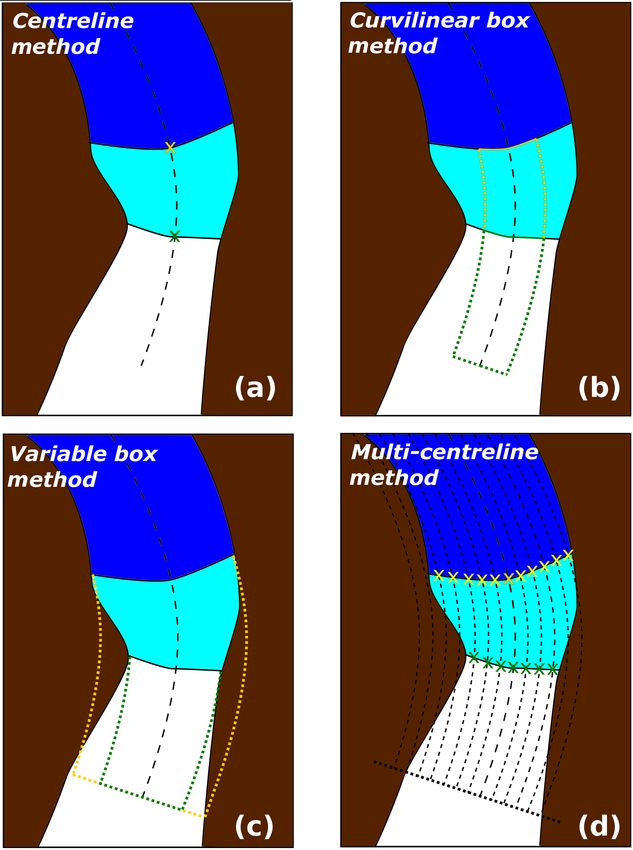
James M. Lea: Rapid mapping and quantification of Earth surface margins                                                                                           553

Table 1. Description of satellites and optional band combinations that are built into GEEDiT. Note that certain user-defined custom band
combinations may have lower resolution.

    Satellite         Imagery        Lifespan                       True colour           False colour            Image       Notes
                      type                                       bands (R-G-B)          bands (R-G-B)         resolution
                                                                                                                    (m)
    Landsat 4         Optical        Jul 1982–Dec 1993                       3-2-1                 5-4-3               30     Gamma: 2
    Landsat 5         Optical        Mar 1984–Jan 2013                       3-2-1                 5-4-3               30     Gamma: 2
    Landsat 7         Optical        Apr 1999–                               3-2-1                 5-4-3               15     Pansharpened from 30 to 15 m using
                                                                                                                              band 8; scan line corrector failure
                                                                                                                              after 31 May 2003; Gamma: 2
    Landsat 8         Optical        Feb 2013–                               4-3-2                 6-5-4               15     Pansharpened from 30 to 15 m
                                                                                                                              using band 8; Gamma: 2
    Sentinel 1A       SAR            1A – Apr 2014–                               –                     –              10     Horiz. transmit/horiz. receive (HH),
    and 1B                           1B – Apr 2016–                                                                           or vert. transmit/vert. receive (VV);
                                                                                                                              Min.: −20; max.: 1
    Sentinel 2A       Optical        2A – Jun 2015–                          4-3-2                 8-4-3               10     Gamma: 2;
    and 2B                           2B – Mar 2017–                                                                           gain: 0.025
Band combinations, gamma options, max./min. ranges and opacity can be varied manually via the “Layers” tab at the top right of the screen.
Imagery is always stored in “Layer 1”.

Video guides that explore the functionality of GEEDiT and                                     A summary of the default parameters used to visualise
GEEDiT Reviewer have also been produced (https://www.                                      both the optical and SAR imagery is given in Table 1. Further
youtube.com/channel/UCboaSHUmNaY7eAeScS0B2_Q).                                             information regarding each satellite image collection can be
                                                                                           obtained by searching for it in the search bar at the top of the
2.1    Image visualisation                                                                 GEE interface.

GEEDiT can visualise imagery from optical imaging plat-
forms as either natural (true colour), false-colour or cus-                                2.2     Output of margin/boundary data
tom band combinations. Sentinel-1 synthetic aperture radar                                 Vector data are output by GEEDiT in decimal degrees for-
(SAR) data can also be visualised as grey scale images (Ta-                                mat so as to be easily read by GIS software and/or subse-
ble 1). SAR data exist in either single- or dual-band polar-                               quently converted to different spatial projections. Key meta-
isation bands, though not every band is collected for every                                data that link each margin to information about the image
scene. To maximise the temporal and spatial coverage for                                   it has been digitised from are appended to each digitised
the tool, GEEDiT will visualise whichever single polarisa-                                 line (see the Supplement readme). This includes each im-
tion band is available (either horizontal transmit/horizontal                              age’s unique path identifier, meaning that results generated
receive (HH) or vertical transmit/vertical receive (VV)) for                               by GEEDiT are directly traceable back to its original image.
both ascending and descending orbits for a particular time                                 This can be achieved using GEEDiT Reviewer, where ex-
and location. The polarisation and type of orbit (ascend-                                  isting datasets can be quality controlled and filtered. If it is
ing/descending) of each SAR image are displayed at the top                                 anticipated that the data digitised in GEEDiT will be anal-
right panel alongside the satellite name, date and image num-                              ysed subsequently in a different GIS environment, it is rec-
ber/total number of images available.                                                      ommended that data are output as GeoJSON files (this is
   Note that the location accuracy of a feature identified in                              the default option), since these can be merged/converted to
Sentinel 1 imagery can be significantly degraded in areas that                             shapefile format using MaQiT. Note that KML/KMZ files do
have undergone several metres of topographic change rela-                                  not always allow metadata to be retained when they are im-
tive to the digital elevation model used for terrain correction                            ported into standard GIS software packages such as ArcGIS
(SRTM 30 for areas < 60◦ latitude; otherwise ASTER DEM).                                   and QGIS using “out of the box” tools. Exporting data from
The scale of geolocation error will also vary depending on                                 GEEDiT/GEEDiT Reviewer in KML/KMZ formats there-
whether the image was acquired during an ascending or de-                                  fore may make subsequent analysis problematic.
scending orbit (see Sect. 4). Care should therefore be taken
in using Sentinel 1 data in such scenarios (e.g. where sig-
nificant surface thinning of a glacier/ice sheet has occurred).                            3     Margin change Quantification Tool – MaQiT
Qualitative checks for this can be achieved by a comparison
of Sentinel 1 data with optical satellite data acquired at a sim-                          MaQiT has been produced to rapidly quantify margin change
ilar time.                                                                                 for use in subsequent analysis (outputs provided as Ex-
                                                                                           cel/OpenOffice compatible csv spreadsheets and as initial

www.earth-surf-dynam.net/6/551/2018/                                                                                    Earth Surf. Dynam., 6, 551–561, 2018
554 James M. Lea: Rapid mapping and quantification of Earth surface margins
plots generated by the tool) and also convert and merge sin- 3.2.1 Centreline method
gle/multiple GeoJSON/shapefile files into a single shapefile.
Although MaQiT uses methods that have been developed for This is the simplest approach to tracking margin change,
the quantification of tidewater glacier margin change (e.g. measuring the linear distance along a centreline between two
Lea et al., 2014), they will be transferable to tracking margin boundaries (e.g. Cook et al., 2005; VanLooy and Forster,
changes in other environments. Each quantification method 2008; Fig. 1a). This approach provides a one-dimensional
has its own benefits and pitfalls, meaning that appropriate measure of change that does not account for the behaviour
method selection should be based primarily on the research of the entire margin; only the point of intersection between
question being asked. the centreline and the margin (Lea et al., 2014). While
this method is simple, the method is best suited to scenar-
ios/research questions where it can be assumed that the mar-
3.1 Installing/running MaQiT
gin is uniformly advancing/retreating or the area of the mar-
Although MaQiT was written in Matlab® , its code has been gin that is of interest is narrow (i.e. a few pixels across). If
compiled into a standalone application (installers available either of these assumptions are not valid, or a higher level
for Windows and Mac) meaning that it can be installed and of detail is required, then an alternative method of tracking
run by users without a Matlab® license and free of any change would be more suitable.
charges. The only prerequisite for this is to download the
free software, Matlab® Runtime, though users should be
prompted once to do this automatically the first time the in-
3.2.2 Curvilinear box method
staller is opened. Users do not require a general Matlab® li-
cense to run MaQiT. This method provides a linear measure of margin ad-
If users do have a general Matlab® license, MaQiT can vance/retreat by defining a box of fixed width spanning the
also be run by copying all the scripts to a single directory centreline that intersects with the margin, before dividing the
and running the MaQiT.m script. This will open MaQiT’s area of this box by its width (Lea et al., 2014; Fig. 1b). The
graphical user interface (GUI), allowing it to be used in a user is required to define the box width. The result provides
similar manner to the standalone application (see Supple- the one-dimensional distance from the start of a centreline
ment readme). The methods used by MaQiT can also be to the mean location of the part of the margin that intersects
run programmatically as Matlab® functions. Where multi- with the box. This method provides a more representative
ple datasets from large numbers of sites exist, this provides width-averaged value of marginal change compared to the
the potential for large-scale rapid analysis. The results gen- centreline method. The method is an extension of the box
erated after the analysis of each location can be accessed via method used by Moon and Joughin (2008) but has the ad-
a data structure named “Results” in the Matlab® workspace vantage that the defined box does not need to be rectilinear
or be written to a csv spreadsheet identical to that produced (i.e. it allows the box to follow potentially non-linear topo-
by the standalone application. MaQiT also makes use of pub- graphic features such as fjords/valleys).
licly submitted functions obtained from the Mathworks File If the defined box width is wider than the margin itself/one
Exchange (Palacios, 2006; D’Errico, 2012a, b, 2013; Dugge, or more edges of the box do not intersect with the margin, the
2015). Copies of these functions are compiled into the stan- box will be “closed” by lines that take the shortest distance
dalone version of MaQiT and are included in the code files from the start/end points of the margin to the box edge. If this
appended to this publication. Instructions regarding the re- scenario is a possibility (i.e. if the box width is greater than
quired inputs for MaQiT and how to use the tool are included that of the margin width), it is important that the centreline
in the Supplement readme file. used extends upstream and downstream of the margins for
a greater distance than the shortest path between the centre-
3.2 Methods of quantifying margin/boundary changes in line and the start/end points of any of the digitised margins
MaQiT (i.e. the centreline should extend up/downstream for more
than twice the width of the longest margin). Failure to do
Four different methods of quantifying margin changes are in-
this may result in errors in the geometry of the boxes used to
cluded in MaQiT, two of which are established approaches
obtain measurements. This can be checked visually using the
that are used in the tracking of tidewater glacier terminus
“Plot output” option in MaQiT, which shows the geometries
change (e.g. Cook et al., 2005; Lea et al., 2014), while two
of each box that is used to quantify margin change. If errors
are new methods designed for the same purpose, though with
of this nature do occur, it is recommended that the user re-
potential wider applications.
draws the centreline using GEEDiT Reviewer, extending the
start/end points of the centreline further up/downstream.
Although this method has the potential to account for a
higher proportion of the margin than the centreline method,
it will not account for the entire margin. It is therefore suit-
Earth Surf. Dynam., 6, 551–561, 2018 www.earth-surf-dynam.net/6/551/2018/James M. Lea: Rapid mapping and quantification of Earth surface margins 555
To ensure the accuracy of results given by this method, it
is important that the start/end points of each margin are at
physically meaningful locations. To ensure the comparabil-
ity of results, this is especially important where it is possi-
ble that the margin will have occupied a given location more
than once. An example of this would be a tidewater glacier,
with physically meaningful start/end points being the two
points at which the glacier margin, sea and land meet (i.e.
the distance between the start and end points of the mar-
gin would give an accurate measurement of glacier width).
If only part of the ice front was digitised, then the method
would give an inaccurate result that may not be comparable
to subsequent observations. Where the method is applied us-
ing arbitrarily/semi-arbitrarily defined start/end points then
the variable box method may over-/under-predict extent de-
pending on how much of and what parts of the margin have
or have not been digitised.
3.2.4 Multi-centreline method
This method extends the centreline method to include multi-
ple centrelines that span the width of a margin. This results in
Figure 1. Methods of margin change quantification that can be ap- many one-dimensional measures of change across the entire
plied in MaQiT. Example shows the retreat of a tidewater glacier
margin width, thus allowing the spatial variability in margin
with ice (white), the former glacier extent (light blue) and open wa-
ter (dark blue). (a) The centreline method takes the linear distance
advance/retreat to be quantified (Fig. 1d). MaQiT visualises
from the start of the centreline to the first point of intersection be- the distance changes that occur as colour change on an x-y
tween the centreline and the margin. (b) The curvilinear box method plot (see Sect. 4). Where the process of interest may occur
generates a box of a user-defined fixed width that is closed at its over timescales longer than the intervals between observa-
downstream edge by the digitised margin, with a one-dimensional tions, it is also possible to define the temporal “window” over
measure of the distance from the start of the centreline obtained which margin changes will be quantified that will improve
by dividing the box area by the box width (note that yellow box data visualisation. For example, if a margin observation ex-
margin also extends to the start of the centreline). (c) The variable ists every 8 days but the research question requires compar-
box method operates on the same principle as the curvilinear box ison of observations made between 30 to 40 days apart, this
method, though box width is automatically defined by MaQiT as the can optionally be defined and MaQiT will automatically fil-
total distance from the end nodes to the centreline. (d) The multi-
ter the observations. These results can also be output to csv
centreline method operates on the same principle as the centreline
method, though multiple, regularly spaced lines are used to build a
files as time–distance tables.
two-dimensional representation of margin change, with the output
using a colour scale to visualise distance. 3.3 Viewing results from MaQiT
The results generated by MaQiT for each method can be vi-
able to apply if the user is interested in obtaining an averaged sualised as a series of plots that are automatically generated
measure of change for a particular section of the margin. by the tool. Due to the nature of each method, the plots used
to visualise the results vary between methods (i.e. the centre-
3.2.3 Variable box method line method does not include a plot to check box geometry
as it does not require using a box). For the centreline and
This method is similar to the curvilinear box method, though curvilinear and variable box methods, there are either three
instead of using a fixed box width, it uses the full width of or four plots shown (e.g. Supplement; Figs. S1–S4). The first
the margin (Fig. 1c). The width of each box is defined as the plot shows all the margins to allow the user to check that
total distance between the start and end nodes of the margin. they have been read in correctly by MaQiT. The second plot
This allows a one-dimensional distance of change to be de- is only included for the curvilinear and variable box meth-
termined that includes the full extent of the digitised margin. ods as it allows the user to check that the box geometries
This has the advantage of accounting for all margin informa- have been constructed correctly and whether redrawing of
tion available, though similar caveats apply to this method as the centreline is necessary. The third plot shows a time se-
the curvilinear box method. ries of distance change of the margin. The multi-centreline
method provides a different output, showing results as a se-
www.earth-surf-dynam.net/6/551/2018/ Earth Surf. Dynam., 6, 551–561, 2018556 James M. Lea: Rapid mapping and quantification of Earth surface margins
Table 2. Description of bands for optical imagery satellites.
Landsat 4 and 5 Landsat 7 Landsat 8 Sentinel 2
Band Band Resolution Band Resolution Band Resolution Band Resolution
number description (m) description (m) description (m) description (m)
1 Blue 30 Blue 30 Ultra blue 30 Coastal aerosol 60
2 Green 30 Green 30 Blue 30 Blue 10
3 Red 30 Red 30 Green 30 Green 10
4 Near-IR 30 Near-IR 30 Red 30 Red 10
5 Shortwave-IR 1 30 Shortwave-IR 1 30 Near-IR 30 Vegetation red edge 20
6 Thermal 120∗ (30) Thermal 60∗ (30) Shortwave-IR 1 30 Vegetation red edge 20
7 Shortwave-IR 2 30 Shortwave-IR 2 30 Shortwave-IR 2 30 Vegetation red edge 20
8 – – Panchromatic 15 Panchromatic 15 Near-IR 10
8A – – – – – – Narrow near-IR 20
9 – – – – Cirrus 30 Water vapour 60
10 – – – – Thermal-IR 1 100∗ (30) Shortwave-IR – cirrus 60
11 – – – – Thermal-IR 2 100∗ (30) Shortwave-IR 20
12 – – – – – – Shortwave-IR 20
∗ indicates where data have been resampled to the resolution given in brackets.
An
Table 3. Summary statistics for the margins digitised from different satellites.
Satellite Margins Mean path Mean Mean number Mean distance
digitised length (m) width (m) of vertices between points (m)
Sentinel 1 (asc.) 39 5643 3357 70.9 82.7
Sentinel 1 (desc.) 39 6204 3316 67.3 95.6
Landsat 8 38 4797 3052 61.6 79.7
Sentinel 2 17 4644 2924 64.1 77.2
Total 133 5869 3203 66.6 91.1
ries of four rows of plots that show (1) marginal change in- license are able to interrogate and subsequently analyse out-
cluding every available observation; (2) marginal change us- put via the Results data structure that is generated and located
ing the defined temporal window (if a temporal window is not in the workspace and/or export data to a csv file. Note that
defined, this plot will be identical to the first plot); (3) abso- the multi-centreline method outputs data as three csv files
lute distance change between observations from one margin showing margin position, margin change from the previous
to the next observation; and (4) rate of margin change be- observation and rate of margin change from the previous ob-
tween observations (e.g. Fig. 5b). The left column of plots servation.
shows changes occurring for the entire margin width, while,
for reference, the right column shows the one-dimensional
results that would otherwise be generated by the centreline 4 Case study – margin change at
method. Breiðamerkurjökull, Iceland
It is strongly recommended for all methods that users view
Breiðamerkurjökull, SE Iceland (64.11◦ N, 16.22◦ W), is an
results generated by MaQiT as a quality control measure of
outlet glacier of the Vatnajökull ice cap that drains into the
both the user’s data and the successful execution of the anal-
tidal lagoon Jökulsárlón (Fig. 2). The calving margin of the
ysis.
glacier was digitised at monthly intervals (where possible)
Users with a standalone MaQiT installation are able to out-
for each of Landsat 8, Sentinel 2 and Sentinel 1 (both ascend-
put results to a csv file for subsequent analysis. Values out-
ing and descending orbits) for January 2014 to January 2018.
put include year, month, date, serial date (i.e. number of days
This allows a broad intercomparison of any systematic biases
since January 0th 0000 AD), margin position on flow line,
that may exist between these platforms in an area that has
margin position relative to the most retreated position, mar-
undergone significant elevation change relative to the digi-
gin change compared to previous observation, rate of change
tal elevation model (DEM) used for terrain correction of the
from previous observation, margin width, and (for box meth-
imagery (Björnsson et al., 2001). A total of 587 images were
ods only) box widths and box area. Users with a Matlab®
viewed during digitisation, with 133 ice fronts digitised in to-
Earth Surf. Dynam., 6, 551–561, 2018 www.earth-surf-dynam.net/6/551/2018/James M. Lea: Rapid mapping and quantification of Earth surface margins 557
Table 4. MaQiT performance metrics.
Method Satellite Number of Total calculation Calculation time
observations time (s) per observation (s)
Centreline method Landsat 8 38 0.49 0.013
Curvilinear box method Landsat 8 38 3.43 0.090
Variable box method Landsat 8 38 2.81 0.074
Multi-centreline method Landsat 8 38 4.56 0.12
Figure 2. Location map and centreline of Breiðamerkurjökull, SE Iceland. Imagery shows a true-colour composite of four Sentinel 2A
scenes acquired on 20 August 2017.
tal. The summary statistics of the digitised margins are given heavily dependent on the research question that the user is
in Table 3. Visualisation and digitisation of the margins were seeking to address. The analysis undertaken here is only to
undertaken in four sessions, taking a total time of 2 h and provide a demonstration of the methods available in MaQiT.
3 min. A metric for the level of detail obtained for a mar-
gin is given as part of the Results/csv output by dividing the 4.1 Case study results
total length of the margin by the number of points digitised
(see mean distance between points, Table 3). Shapefiles of 4.1.1 Intercomparison of results from different satellites
the combined Landsat 8 and Sentinel 2 records of margin
The curvilinear box method (width: 2000 m) was used to
change are included as a Supplement as example data.
illustrate whether any systematic differences exist between
Once digitisation of the ice margins was complete, MaQiT
margins digitised from different satellites (Fig. 3). Results
was used to convert and merge the GeoJSON files gener-
show that while similar patterns and magnitudes of change
ated by GEEDiT to a single shapefile. The appended Sup-
are given for each satellite, margins digitised from Sen-
plement data can also be visualised in GEEDiT Reviewer by
tinel 1 imagery show clear under- and overestimation of mar-
copy and pasting the path users/Jmleaglacio/Breida_L8_S2
gin extent (relative to Sentinel 2 and Landsat 8 imagery)
into the tool.
for descending and ascending orbits respectively. One-to-one
It should be emphasised that the method of margin change
matches in results are not expected as image acquisitions for
quantification that should be used for this type of data is
the different satellites did not always fall on the same day,
www.earth-surf-dynam.net/6/551/2018/ Earth Surf. Dynam., 6, 551–561, 2018558 James M. Lea: Rapid mapping and quantification of Earth surface margins
10 600 600
Sentinel 1 - ascending orbit Centreline method
Sentinel 1 - descending orbit Curvilinear box method (width = 1000 m)
Landsat 8 Curvilinear box method (width = 2000 m)
Sentinel 2 Variable box method
10 400 500
400
Distance from start of centreline (m)
most recent observation (m)
10 200
Margin position relative to
300
10 000
200
9800
100
9600
0
9400
-100
9200 -200
2013 2014 2015 2016 2017 2018 2019 2013 2014 2015 2016 2017 2018 2019
Year Year
Figure 3. Intercomparison of monthly margin positions at Figure 4. Intercomparison of results from different margin quantifi-
Breiðamerkurjökull given by the curvilinear box method (width: cation methods applied to the Landsat 8 monthly record of margin
2000 m) digitised from different satellites. positions at Breiðamerkurjökull.
while the margin of Breiðamerkurjökull is known to flow 4.2.1 One-dimensional measures of margin change
rapidly (> 5 m d−1 ; Voytenko et al., 2015), meaning that the
margin has the potential to be highly dynamic over short The centreline, curvilinear box and variable box methods
timescales (cf. Benn et al., 2017). provide one-dimensional measures of margin change (i.e.
Though results from Sentinel 2 and Landsat 8 are broadly how far advanced/retreated a margin is relative to the dis-
comparable, Fig. 3 illustrates that for Sentinel 1 imagery tance along a centreline). Figure 4 shows that each of the
there can be significant mismatch in areas where significant methods record similar overall patterns of change (i.e. re-
elevation change has occurred relative to the DEM used for treat), though at times diverge from each other depending
initial terrain correction. In environments where consider- on method/parameter choice. In particular, the centreline
able elevation change has not occurred the mismatch should method displays a high degree of variability (e.g. 2015–
be less, though margins from ascending and descending or- 2018) as it reflects margin change in an extremely localised
bits (automatically appended by GEEDiT to margin meta- area. This is in contrast to the other methods that provide re-
data) should still be checked for systematic biases. Due to sults that are more representative of the margin as a whole.
the “oblique looking” nature of Sentinel 1 image acquisitions It should also be noted that while each method generally
(compared to “vertical looking” for optical satellite imagery), agrees on the sign of margin change (i.e. advance or re-
the magnitude of mismatches in areas of elevation change are treat), this is not always the case. In general, methods that
likely to be variable across an image. account for larger proportions of the margin (i.e. the variable
The mismatches shown in these results demonstrate that box and curvilinear box method (width: 2000 m)) are more
considerable care should be taken in combining observations likely to disagree with methods that account for less of the
from Landsat/Sentinel 2 imagery with Sentinel 1 imagery. margin (i.e. centreline and curvilinear box methods (width:
1000 m)). This highlights the importance of the need to care-
fully select method/parameter choice with respect to the re-
4.2 Intercomparison of methods for quantifying margin
search question that is being addressed.
change
Observations of margin change at Breiðamerkurjökull ob- 4.2.2 Multi-centreline method
tained from Landsat 8 are used to demonstrate the different
methods of margin change quantification included in MaQiT. The multi-centreline method provides a two-dimensional
representation of margin change, highlighting regions of the
margin that are more susceptible to advance/retreat, in ad-
dition to the timing and magnitude of this. It also pro-
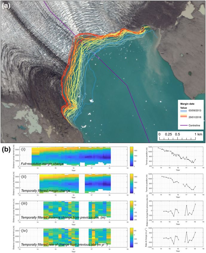
Earth Surf. Dynam., 6, 551–561, 2018 www.earth-surf-dynam.net/6/551/2018/James M. Lea: Rapid mapping and quantification of Earth surface margins 559 Figure 5. Margin migration for monthly Landsat 8 observations of Breiðamerkurjökull shown as a time series (a) cartographically and (b) as results from the multi-centreline method. Panel (b) has four rows of plots showing (i) the margin position for all available observations relative to the most retreated position across the margin; (ii) margin position observations separated by at least 60 days and a maximum of 120 days (these values are user-defined); (iii) total distance change between observations; and (iv) rate of change of margin in m yr−1 . Right-hand column of plots displays results of the centreline method for comparison. www.earth-surf-dynam.net/6/551/2018/ Earth Surf. Dynam., 6, 551–561, 2018
560                                                 James M. Lea: Rapid mapping and quantification of Earth surface margins

vides a means of visualising two-dimensional change as a             where significant elevation change may have occurred rela-
time series rather than relying on maps of margin change             tive to the DEM that is used for terrain correction of imagery
that may otherwise be difficult to interpret in a meaning-           in Google Earth Engine.
ful way (e.g. Fig. 5a). For the case study, observations were           Intercomparison of the two existing and two new meth-
obtained at approximately monthly intervals, though the              ods of margin change quantification available in MaQiT il-
method has been applied so as to highlight changes over sea-         lustrate the potential for obtaining potentially substantial dif-
sonal timescales (60 to 120 days). Results show that the cen-        ferences in margin change values when analysing the same
tre of Breiðamerkurjökull’s margin is consistently the most          data. This highlights the importance of users selecting the
retreated (Fig. 5bi, ii) and that there is little seasonal consis-   most suitable margin quantification method for their particu-
tency across the entire margin as to whether it advances or          lar research problem. The new multi-centreline method also
retreats and at what rate (Fig. 5biii, iv).                          provides a means of visualising margin change as a time se-
                                                                     ries potentially in a clearer manner than is possible carto-
4.3    MaQiT performance                                             graphically. While these techniques have predominantly been
                                                                     developed for the quantification of tidewater glacier margin
Table 4 shows performance metrics of each method from the            change, they could also be useful for researchers investi-
standalone version MaQiT. The speed at which users would             gating coastal change, dune migration and vegetation extent
be able to complete comparable analysis without MaQiT is             changes amongst other areas of Earth surface science.
highly dependent on an individual’s existing GIS and/or cod-
ing competence. However, for those without coding skills
and entry level GIS training, it may take a user several min-        Data availability. Links to GEEDiT and GEEDiT Reviewer and
utes to obtain a single value that quantifies the position of        downloads for MaQiT can be found at the following website: www.
one margin. MaQiT, therefore, provides a potentially major           liverpoolGEE.wordpress.com.
improvement in the efficiency with which users can anal-
yse their data. Results produced by MaQiT are also guaran-
teed to be methodologically consistent and replicable. This
                                                                     The Supplement related to this article is available online
makes MaQiT highly suited to the (re-)analysis of repository
                                                                     at https://doi.org/10.5194/esurf-6-551-2018-supplement.
datasets of margin change.

5     Summary
                                                                     Competing interests. The author declares that there is no con-
Together GEEDiT, GEEDiT Reviewer and MaQiT provide
                                                                     flict of interest.
simple tools for rapid satellite image visualisation, explo-
ration and initial assessment (via notes appended to meta-
data), digitisation of margins from imagery, review and filter-      Acknowledgements. The author wishes to thank William
ing of existing datasets, and quantification of their changes        Armstrong and Mauri Pelto for constructive reviews that have
via multiple methods. They dramatically improve the effi-            helped to improve both the manuscript and the tools presented in
ciency with which these analyses can be undertaken and               this paper. The author also wishes to thank Stephen Brough and
the accessibility of these data to researchers both with and         Adam Hepburn for comments and suggestions on GEEDiT. Also
without knowledge of coding. The lack of the requirement             acknowledged are Jack Boitier, John Cordall, Phoebe Cox, Elaine
to download, process and store imagery on a user’s com-              Crimmins, Ajjay Dhesi and Thomas Hutton, who extensively
puter, coupled with simple GUIs and no fee-paying licens-            tested an earlier version of MaQiT as part of their undergraduate
ing requirements also improves the accessibility to these data       dissertations.
through the removal of traditional barriers to entry associated
                                                                     Edited by: David Lundbek Egholm
with remote sensing and GIS. The tools are therefore suitable
                                                                     Reviewed by: Mauri Pelto and William Armstrong
for users ranging from high school students to academics.
   GEEDiT provides flexibility for the way in which imagery
is visualised (i.e. true-colour, false-colour and custom band
combinations), while MaQiT gives users the flexibility to            References
rapidly quantify and output measures of margin change. The
                                                                     Benn, D. I., Åström, J., Zwinger, T., Todd, J., Nick, F. M., Cook,
case study of the calving glacier Breiðamerkurjökull high-
                                                                       S., Hulton, N. R., and Luckman, A.: Melt-under-cutting and
lights the potential for mismatch between imagery collected            buoyancy-driven calving from tidewater glaciers: new insights
via ascending/descending orbits of Sentinel 1 relative to opti-        from discrete element and continuum model simulations, J.
cal imagery satellites such as Landsat and Sentinel 2. Conse-          Glaciol., 63, 691–702, 2017.
quently users should take care in combining margin records           Bevan, S. L., Luckman, A. J., and Murray, T.: Glacier dynamics
from Sentinel 1 with those of Landsat/Sentinel 2, especially           over the last quarter of a century at Helheim, Kangerdlugssuaq

Earth Surf. Dynam., 6, 551–561, 2018                                                      www.earth-surf-dynam.net/6/551/2018/
James M. Lea: Rapid mapping and quantification of Earth surface margins 561 and 14 other major Greenland outlet glaciers, The Cryosphere, Lea, J. M., Mair, D. W. F., and Rea, B. R.: Evaluation of existing and 6, 923–937, https://doi.org/10.5194/tc-6-923-2012, 2012. new methods of tracking glacier terminus change. J. Glaciol., 60, Björnsson, H., Pálsson, F., and Guðmundsson, S.: Jökulsárlón at 323–332, 2014. Breiðamerkursanður, Vatnajökull, Iceland: 20th century changes Lea, J.: University of Liverpool Google Earth Engine Tools/MaQiT, and future outlook, Jökull, 20th century changes and future out- available at: bewww.liverpoolGEE.wordpress.com, last access: look, Jökull, 50, 1–18, 2001. 12 July 2018. Bunce, C., Carr, J. R., Nienow, P. W., Ross, N., and Killick, R.: Ice Lynch, C., Barr, I. D., Mullan, D., and Ruffell, A.: Rapid glacial re- front change of marine-terminating outlet glaciers in northwest treat on the Kamchatka Peninsula during the early 21st Century, and southeast Greenland during the 21st century, J. Glaciol., 1– The Cryosphere, 10, 1809–1821, https://doi.org/10.5194/tc-10- 13, 2018. 1809-2016, 2016. Carr, J. R., Stokes, C. R., and Vieli, A.: Threefold increase in Moon, T. and Joughin, I.: Changes in ice front position on Green- marine-terminating outlet glacier retreat rates across the Atlantic land’s outlet glaciers from 1992 to 2007, J. Geophys. Res.-Earth Arctic: 1992–2010, Ann. Glaciol., 58, 72–91, 2017. Surf., 113, https://doi.org/10.1029/2007JF000927, 2008. Cook, A. J., Fox, A. J., Vaughan, D. G., and Ferrigno, J. G.: Re- Motyka, R. J., Cassotto, R., Truffer, M., Kjeldsen, K. K., Van treating glacier fronts on the Antarctic Peninsula over the past As, D., Korsgaard, N. J., Fahnestock, M., Howat, I., Langen, half-century, Science, 308, 541–544, 2005. P. L., Mortensen, J., and Lennert, K. Asynchronous behavior D’Errico, J.: Arclength function, available at: https://uk.mathworks. of outlet glaciers feeding Godthåbsfjord (Nuup Kangerlua) and com/matlabcentral/fileexchange/34871-arclength (last access: 5 the triggering of Narsap Sermia’s retreat in SW Greenland, J. July 2018) 2012a. Glaciol., 63, 288–308, 2017. D’Errico, J.: interparc function, available at: https://uk.mathworks. Palacios, R.: Deg2utm function, available at: https://uk.mathworks. com/matlabcentral/fileexchange/34874-interparc (last access: 5 com/matlabcentral/fileexchange/10915-deg2utm?focused= July 2018), 2012b. 5073379&tab=function (last access: 5 July 2018), 2006. D’Errico, J.: Distance2curve function, available at: Planet Labs Inc.: Planet Image Explorer, available at: https://www. https://uk.mathworks.com/matlabcentral/fileexchange/ planet.com/, accessed 9 February 2018. 34869-distance2curve, (last access: 5 July 2018), 2013. Roelfsema, C., Kovacs, E. M., Saunders, M. I., Phinn, S., Lyons, Dugge, J.: Jdugge/xy2sn, available at: https://uk.mathworks.com/ M., and Maxwell, P.: Challenges of remote sensing for quantify- matlabcentral/fileexchange/39796-jdugge-xy2sn (last access: 5 ing changes in large complex seagrass environments, Estuarine, July 2018), 2015. Coast. Shelf Sci., 133, 161–171, 2013. Fitzpatrick, A. A. W., Hubbard, A. L., Box, J. E., Quincey, D. J., van Sinergise: Sentinel Hub Earth Observation Explorer, https:// As, D., Mikkelsen, A. P. B., Doyle, S. H., Dow, C. F., Hasholt, sentinel-hub.com/explore/eobrowser, last access: 9 February B., and Jones, G. A.: A decade (2002–2012) of supraglacial lake 2018. volume estimates across Russell Glacier, West Greenland, The Voytenko, D., Dixon, T. H., Howat, I. M., Gourmelen, N., Lem- Cryosphere, 8, 107-121, https://doi.org/10.5194/tc-8-107-2014, bke, C., Werner, C. L., De La Peña, S., and Oddsson, B.: Multi- 2014. year observations of Breiðamerkurjökull, a marine-terminating Gorelick, N., Hancher, M., Dixon, M., Ilyushchenko, S., Thau, D., glacier in southeastern Iceland, using terrestrial radar interfer- and Moore, R.: Google Earth Engine: Planetary-scale geospatial ometry, J. Glaciol., 61, 42–54, 2015. analysis for everyone, Remote Sens. Environ., 202, 18–27, 2017. Kuenzer, C., van Beijma, S., Gessner, U., and Dech, S.: Land sur- face dynamics and environmental challenges of the Niger Delta, Africa: Remote sensing-based analyses spanning three decades (1986–2013), Appl. Geogr., 53, 354–368, 2014. www.earth-surf-dynam.net/6/551/2018/ Earth Surf. Dynam., 6, 551–561, 2018
You can also read