Modeling and forecasting the COVID-19 temporal spread in Greece: an exploratory approach based on complex network defined splines - arXiv
←
→
Page content transcription
If your browser does not render page correctly, please read the page content below
Preprint
Modeling and forecasting the COVID-19 temporal spread
in Greece: an exploratory approach based on complex
network defined splines.
Konstantinos Demertzis1*, Dimitrios Tsiotas1,2,3, and Lykourgos Magafas1
 1
   Laboratory of Complex Systems, Department of Physics, Faculty of Sciences, International Hellenic University,
   Kavala Campus, St. Loukas, 65404, Greece; kdemertzis@teiemt.gr; magafas@teikav.edu.gr;
 2
   Department of Regional and Economic Development, Agricultural University of Athens, Greece, Nea Poli,
   Amfissa, 33100, Greece; tsiotas@aua.gr;
 3
   Department of Planning and Regional Development, University of Thessaly, Pedion Areos, Volos, 38334, Greece;
   tsiotas@uth.gr;
 * Correspondence: kdemertzis@teiemt.gr;
 Received: date; Accepted: date; Published: date

 Abstract: Within the complex framework of anti-COVID-19 health management, where the criteria of
 diagnostic testing, the availability of public-health resources and services, and the applied anti-COVID-19
 policies vary between countries, the reliability and the accuracy in the modeling of temporal spread can
 be proven effective in the worldwide fight against the disease. This paper applies an exploratory
 time-series analysis to the evolution of the disease in Greece, which currently suggests a success story
 of COVID-19 management. The proposed method builds on a recent conceptualization of detecting
 connective communities in a time-series and develops a novel spline regression model where the knot
 vector is determined by the community detection in the complex network. Overall, the study
 contributes to the COVID-19 research by proposing a free of disconnected past-data and reliable
 framework of forecasting, which can facilitate decision-making and management of the available health
 resources.

 Keywords: COVID-19 coronavirus pandemic; outbreak; modeling; prediction; regression splines;
 modularity optimization algorithm.

1. INTRODUCTION
The coronavirus disease 2019, abbreviated as COVID-19, is a contagious disease caused by the severe
acute respiratory syndrome coronavirus 2 (SARS-CoV-2), which frequently causes fever, cough, and
dyspnea, and less frequently muscle pains and neck-related problems (Ahmed et al., 2020; Lescure et al.,
2020; Xu et al., 2020b). The virus is mainly transmitted to humans through respiratory channels and the
majority of patients is asymptomatic or has soft symptoms to the disease, but certain cases develop
either pneumonia, the worst aspect of which is the fatal Acute Respiratory Distress Syndrome (ARDS), or
multi-organic deficiency (Xu et al., 2020b). The time from exposition to the appearance of symptoms
ranges from 2 to 14 days, with a 5-day average, the long range of which is affected by the relevance of
the disease, in its asymptomatic or soft symptomatology aspect, with the common cold (Fang et al.,
2020; Heymann and Shindo, 2020). An amount of 25% of - 30% of patients worsens after the 14th day of
exposition, showing respiratory infection, whereas an amount of 83% of patients develops lymphopenia
(Tan et al., 2020). The disease is also observed in children, by usually with soft symptoms (Liu et al., 2020;
Qiu et al., 2020).
     The COVID-19 is detected either by laboratory methods, usually by the method of Polymerase Chain
Reaction (PCR) (Bai et al., 2020), where the sample is received from the rhino-laryngology region, or just
by clinical methods, by evaluating combinations of symptoms (at least of two major), danger-factors,
and indications of the chest radiogram, in conjunction with the history of the patients’ contacts and
movements (Bai et al., 2020; Ye et al., 2020). Currently, since no vaccine or cure for the disease is
available (Lurie et al., 2020), the major efforts of the medical community are focusing on the
management of symptoms, while of the governance are focusing on the management of public-health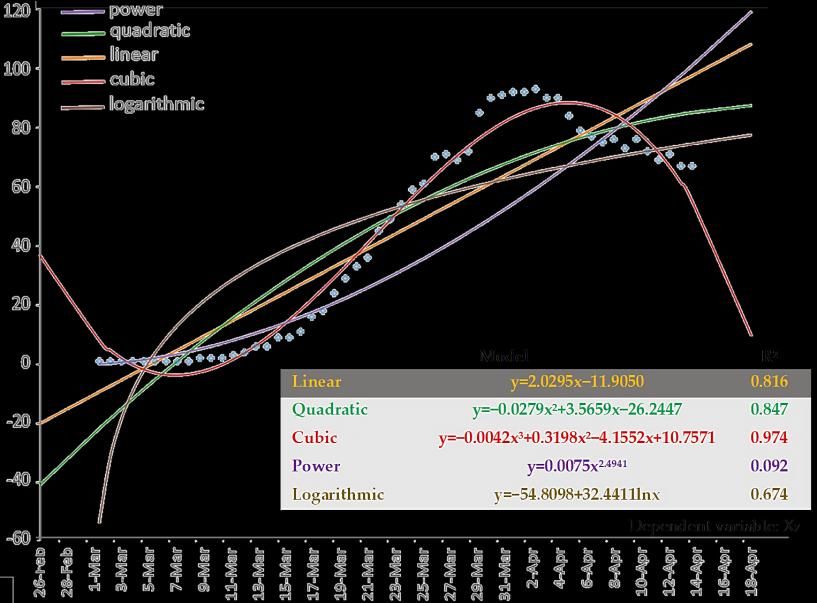
PREPRINT                                                                                               2 of 16

resources and on the prevention management of the disease. Within the context that COVID-19 is a
particularly airborne contagious disease, medical directives to the public highlight the need for careful
personal body hygiene, while government policies (Tsiotas and Magafas, 2020) impose severe
restrictions of mobility, gathering, transportation, and trade activities.
      In particular, starting to the mid of December 2019, when COVID-19 emerged in the city of Wuhan,
China, up to the 19th of April 2020, the disease was spread up to 210 countries, causing 2,408,123
infections and 165,105 deaths (Roser and Ritchie, 2020). Despite that its spatiotemporal pattern
specializes amongst countries worldwide, it is a common feature that the pandemic shows scaling trends
worldwide (with couple exemptions the cases of South Korea and China) without illustrating a tendency
of stabilization. For instance, up to the 19th of April 2020, North America recorded 43,369 deaths and
820,749 infections, South America 3,850 deaths and 82,310 infections, Asia 14,801 deaths and 383,542
infections, Africa 1,128 deaths and 22,992 infections, and Oceania 83 deaths and 8,150 infections (Our
World in Data, 2020; Worldometers, 2020). On the other hand, Europe is more hardly affected by the
pandemic because, although it counted the half infections (1,089,659), it recorded over the 60% of the
worldwide deaths (101,859), from which an amount of 78.4% (72,196 deaths) were in Italy (23,660), Spain
(20,453), France (19,718), and United Kingdom (16,060) (Our World in Data, 2020; Worldometers, 2020).
      On the contrary to the worldwide and European status of COVID-19, Greece has a proportion of 240
confirmed infections per million of population, which is almost 35% lower than the global average, which
is about 370 infections per million, and 85% than the European average, which is about 1330 infections
per million (Our World in Data, 2020; Worldometers, 2020). Within the context of promising a success
story in the fight against the disease, this paper develops a novel non-parametric method for the
modeling of the evolution of the Greek COVID-19 infection-curve that can facilitate to more accurate
forecasting. The proposed method builds on a recent conceptualization of detecting communities of
connectivity in a time-series (Tsiotas and Magafas, 2020) and develops a novel model based on the
Regression Splines algorithm that is more accurate and reliable in forecasting. The overall approach
provides insights of good policy and decision-making practices and management that can facilitate
decision-making and management of the available health resources in the fight against COVID-19.
      The remainder of the paper is organized as follows; Section 2 reviews the literature in the current
analysis of COVID-19 temporal spread, Section 3 applies a descriptive analysis of COVID-19 in Greece,
Section 4 describes the methodological framework of the proposed method, Section 5 shows the results
of the analysis and discusses them within the context of public-health management and practice, and,
finally, in Section 6 conclusions are given.

2. LITERATURE REVIEW
The work of Xu et al (2020) is a detailed presentation of COVID-19 records that are extracted from
national, regional, municipal health-reports, and web information aiming to contribute to the
decision-making for the public health with insightful primary information. This work focuses more on the
recording than on the analysis of cases and therefore it exclusively contributes to COVID-19 research as
an archive of statistical data. The work of Sarkodie and Owusu (2020) is an insightful time-series analysis
examining the interconnection between deaths and infected cases, based on four health indicators of
COVID-19, in China. The analysis uses cross-sectional dependence, endogeneity, and unobserved
heterogeneity estimation methods, and detects a linear relationship between COVID-19 attributable
deaths and confirmed cases whereas a non-linear relationship ruling the nexus between recovery and
confirmed cases. This work contributes to the literature with an interesting case-study that is by default
restricted to the case of China, to the limited number of indicators used in the analysis, and to the limited
time-series dataset that does not facilitate reliable forecasting. Next, the work of Anastassopoulou et al.
(2020) proposes a heuristic method for estimating basic epidemiologic parameters, for modeling, and
forecasting the COVID-19 spread based on available epidemiologic data. Their approach suggests a
reverse forecasting process that builds on spreading scenarios, which reproduce the confirmed cases,
and it develops a directed tendency which cannot promise a reliable basis for forecasting. Also,
Petropoulos and Makridakis (2020) study the temporal-spread of the disease based on exponential
smoothing modeling. Although interesting, this approach is restricted to the insufficient number of past
data, on which their exponential model and promises to forecast the tendency of the COVID-19 future
spreading model of illness of past, while the fitted curve is calibrated and smoothened in accordance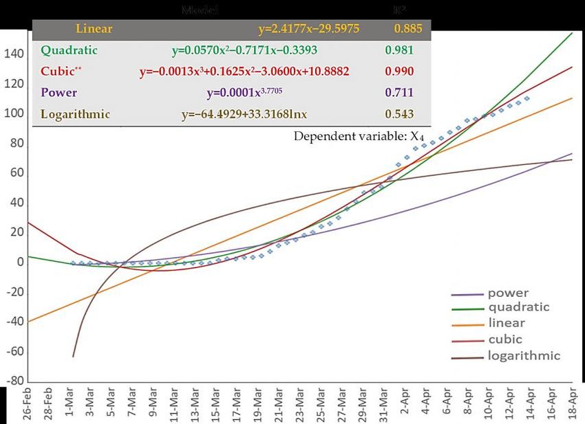
PREPRINT                                                                                               3 of 16

with the foregoing available cases of other countries. Moreover, Fong et al. (2020) presented an
interesting forecasting model, based on a polynomial neural network with corrective feedback, which is
capable to forecast with satisfactorily accuracy, even in cases of insufficient data availability. Although
interesting, this approach should be further tested and compared with alternative established
algorithms of similar good accuracy by taking into consideration more than the accuracy criterion for the
comparison.
      On the other hand, due to the diversity that the phenomenon has in different countries, many
researchers were focused on national case-studies of COVID-19 instead of the global case. For instance,
Mahase (2020) demonstrated the changes in statistical data of the United Kingdom after the application
of the anti-COVID-19 social distance policies. In Italy, many studies were conducted for the modeling of
the pandemic (Giuliani et al., 2020; Livingston and Bucher, 2020; Remuzzi and Remuzzi, 2020), due to
fatal outbreak that the disease had in the country, which attracted the global attention. The work of
Giuliani et al. (2020) is a characteristic early study of modeling the spatiotemporal spread of COVID-19 in
Italy, where the analysis builds on statistical modeling but without testing the statistical significance of
the research hypothesis. Within the context of epidemiologic research, this incompleteness restricts the
contribution of this interesting approach, provided that in epidemiologic studies the goal is to develop
an occurrence function (as a measure of association) quantifying a cause-effect relation between a
determinant (cause) and its result (effect) and therefore the major concern is to test whether this
cause-effect relation is statistically significant.
      Greece is an example of timely response in the application of anti-COVID-19 policies that are
currently have been proven effective in keeping the infected cases and deaths at relatively low levels
(Roser and Ritchie, 2020; Xu et al., 2020; Tsiotas and Magafas, 2020). In particular, the first infection
emerged in the country on February 26th, 2020, and just three days later the state began applying several
policies for the control of the disease (Tsiotas and Magafas, 2020). This timely response have led Greece
to be currently considered as a successful case in anti-COVID-19 management, comparatively both to the
European and the global cases (Roser and Ritchie, 2020; Xu et al., 2020). At the time that Greece started
attracting the global attention, Tsiotas and Magafas (2020) proposed a novel complex network analysis
of time-series, based on the visibility algorithm (Lacasa et al., 2008; Tsiotas and Charakopoulos, 2020), for
the study of the Greek COVID-19 infection curve. The authors showed that the evolution of the disease in
Greece went through five stages of declining dynamics, where saturation trends (represented by a
logarithmic pattern) emerged after the 33rd day (29/04/2020). Within the context that Greece promises a
success story and an insightful case study, both in epidemiologic and in anti-COVID-19 policy terms, this
paper builds on the very recent work of Tsiotas and Magafas (2020) and advances the time-series
modeling and forecasting by developing a model based on the Regression Splines algorithm that is more
capable to provide accurate predictions of future trends.

3. DESCRIPTIVE ANALYSIS OF COVID-19 IN GREECE
The disease of COVID-19 emerged in Greece on 26 February 2020, almost two months after its global
emergence (Tsiotas and Magafas, 2020). As it can be observed in Fig.1, within the 54 first days of the
pandemic (until 19 April), Greece recorded 2,235 confirmed infected cases (Worldometers, 2020), from
which an amount of 56% are men, 25.5% (570 cases) are related with traveling abroad, 42.2% (943 cases)
are linked with other confirmed cases, whereas the others are untracked and are still undergoing
investigation (NPHOG, 2020). The average age of cases is 49 years (ranging from 1 day until 102 years
old), whereas the medium death age is 74 years (ranging from 39 to 95 years) (NPHOG, 2020).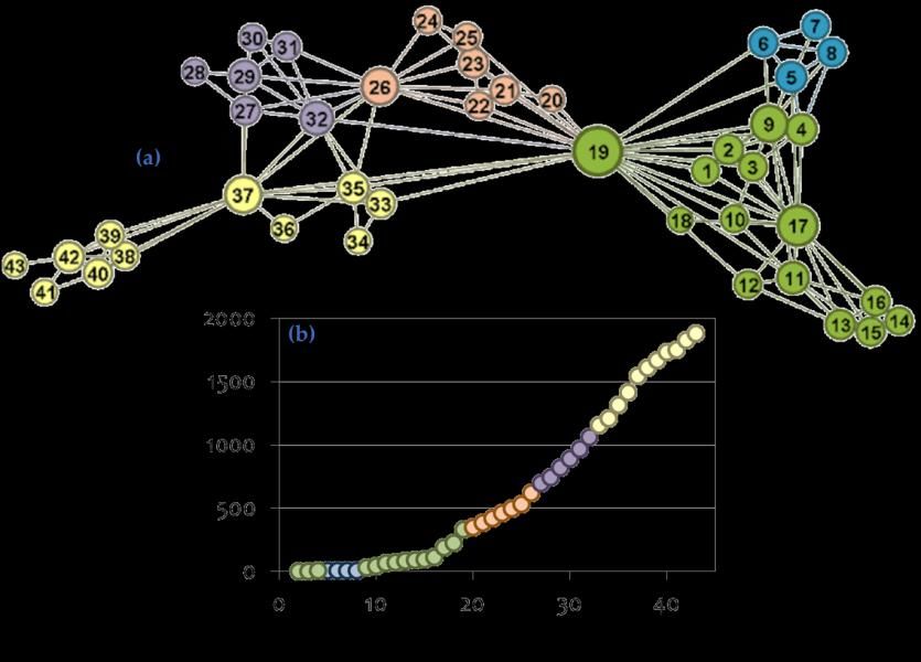
PREPRINT 4 of 16
Fig.1. The time-series of the COVID-19 infection curve in Greece, for the period 15 Feb 20 - 18 Apr 20. The first infection emerged on
26 Feb 20 (and recorded on 27 Feb 20) (data source: Worldometers, 2020).
In numeric terms, Greece is worldwide at the 58th place in number of infected cases and at the 46th
place in number of deaths (Worldometers, 2020), while, in Europe, is at the 25th place in number of cases
and at the 22th place in deaths. In per capita terms, Greece has currently 13 deaths per million of
population (Worldometers, 2020), while the global average is above 16 deaths per million of residents
(Our World in Data, 2020). Also, with 67 patients being under a serious-critical situation, Greece is
worldwide at the 37th place and at the 20th place in Europe (NPHOG, 2020; Our World in Data, 2020;
Worldometers, 2020). In terms of testing, Greece has conducted 50,771 tests and takes the 56th place
worldwide and the 23rd place in Europe (NPHOG, 2020; Our World in Data, 2020; Worldometers, 2020).
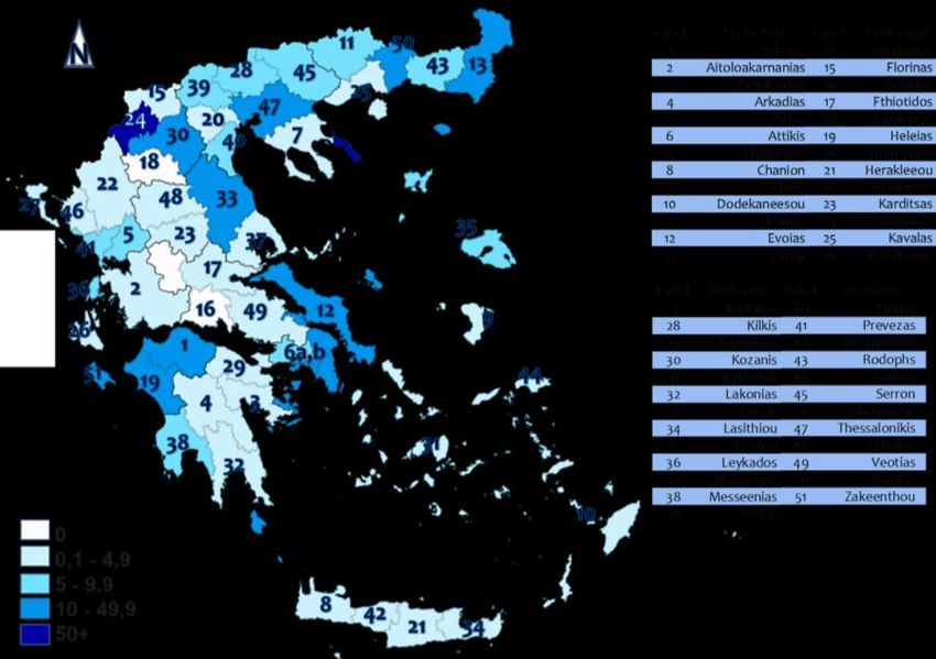
The geographic distribution of the confirmed infected cases in Greece are shown in the map of Fig.2
(NPHOG, 2020), where it can be observed that the majority of infections are concentrated in the
metropolitan prefectures of Attiki (6) and Thessaloniki (47), along a vertical axis configured by the
prefectures of Kastorias (24), Kozanis (30), and Larissas (33), at central Greece, in the prefecture of
Euvoias (12), in the prefectures of Xanthis (50) and Evrou (13), at the north-east country, and at the
prefectures of Achaias (1), Heleias (19), and Zakenthou (51), at the south-west Greece, the majority of
which are transportation (road, maritime, and air transport) centers.
Fig.2. Infected cases per million in Greece (source: NPHOG, 2020)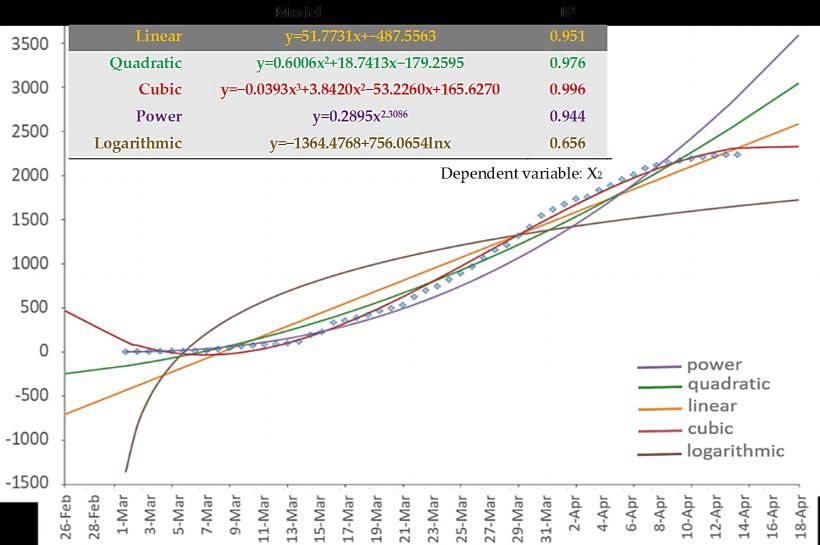
PREPRINT                                                                                                                       5 of 16

      Also, Greece is worldwide in the 68th place and in the 26th place in Europe regarding the number of
patients recovered from COVID-19 (NPHOG, 2020; Our World in Data, 2020; Worldometers, 2020). The
daily and cumulative infections of COVID-19 in Greece are shown in Fig.3.

Fig.3. The time-series of the COVID-19 death curve in Greece, for the period 15 Feb 20 - 18 Apr 20. The first death was recorded on 12
                                            Mar 20 (data source: Worldometers, 2020).

     Next, Fig.4 shows the evolution of the confirmed infected cases in Greece comparatively to the
respective recorded deaths. The vertical axis of the diagram is graded at the logarithmic scale, where
linear segments illustrate exponential growth of the disease (the slope of the linear growth is
proportional to the size of the exponent). As it can be observed, the almost constant offset between the
two curves implies that the number of infections and the number of deaths of COVID-19 in Greece are
correlated. This interprets that these two indicators follow a similar growth pattern, which is in line with
the shape of the curves shown in Figures 1 and 3. Also, a particularly promising observation is the
declining growth rates shown in Fig.4 for both the infection and death curves. However, these
observations will be statistical tested at a following part of the analysis.

Fig.4. Comparative diagram with the time-series of the COVID-19 infection cases versus the recorded deaths in Greece (data source:
                                                           NPHOG, 2020).

     Next, Fig.5 is an aggregate diagram showing the evolution of COVID-19 confirmed (total) cases, new
infections, deaths, and recovered on official data extracted from the Greek Ministry of Health (NPHOG,
2020).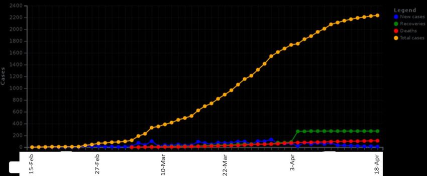
PREPRINT                                                                                                                   6 of 16

Fig.5. The aggregate time-series of the COVID-19 in Greece, showing the number of confirmed (total) cases, new infections, deaths,
                      and recoveries, for the period 15 Feb 20 - 18 Apr 20 (data source: Worldometers, 2020).

      Within the context of the global outbreak of the disease, the previous descriptive analysis illustrates
that Greece suggests a good example for its COVID-19-related sizes, which keep the country at the last
places both in the European and the global ranking. However, this good performance has been the result
of the timely response and application of anti-COVID-19 policies in Greece (Tsiotas and Magafas, 2020),
including a set of measuring of social distancing to prevent the spreading of the disease, In particular,
the first anti-COVID-19 policies in Greece were applied after the confirmation of the first three infected
cases, which were dated on the 27th of February 2020. On that day, all carnival events were cancelled to
prevent an outbreak of the disease. On the 10th of March, the number of total cases reached 89 (MOHG,
2020), the tracking of which revealed that they were mainly related either with travellers originating
from Italy or with pilgrims returned from religious excursion to Israel of with travelers from Egypt, along
with their contacts (MOHG, 2020). On that day, the government announced to the population directives
related to personal hygiene, social distancing, and prevention, while the anti-COVID-19 measures up to
then were optional and applicable at the local level (and particularly at the regions with infected cases,
such as Heleias-19, Achaias-1 and Zakynthou-51), mainly concerning local suspension of schools, school
excursions abroad, and cultural events (Tsiotas and Magafas, 2020). However, on 10th of March, due to
the spreading of the disease to multiple regions and due to the disobedience of the citizens to conform
with the measures, the government applied more active measures and proceeded to the national
suspension of all educational structures (at all ranks), and couple of days later, on the 12th and 13th of
March, it proceeded to the suspension of cafeterias, bars, museums, malls and trade centers, sport
activities, restaurants, and relevant (MOHG, 2020). On 16th of March, all commercial shops were
suspended at the national level, two villages in the regions of Kozani (30) were put into quarantine, and
all doctrine and religious activities were suspended (MOHG, 2020). The only active businesses and firms
exempted from these measures were primary need suppliers, such as bakeries, supermarkets,
pharmacies, and health private services (MOHG, 2020). Aiming to support the anti-COVID-19 policy of
social distancing, the government announced, on 18th and 19th of March, a set of measures of 10 billion
Euros (€) budgest, which either concerned taxation benefits or regulations or subsidies, for the support
of the economy, of companies, and of workers offended by the suspensions and by the social distancing
(MOHG, 2020). On the 23rd of March 2020 the government announced national restrictions in
transportation, with exemptions the commuting to work, movements for supplies of food, medicines,
medical services, and health-gymnastics. However, these exemptions should be documented by
identification papers, such as the ID-card or passport and an affirmation paper stating the purpose of
movement (MOHG, 2020). At their circulation, provided that he is related with somebody of the
acceptable exceptions, the citizens will be supposed to bring their police identity or the passport, as well
as some type certification of proportionally aim of locomotion. This measure was applicable until 27th of
April 2020 and it was extended until 4th of May 2020 (MOHG, 2020).
      In the fight against the disease, the development of more accurate and reliable models in terms of
description and prediction can help policy makers to better conceptualize the pandemic and apply
proper and more effective policies. Towards this direction, this paper proposes a novel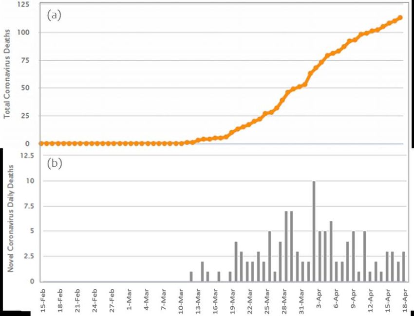
PREPRINT                                                                                                                                        7 of 16

complex-network-based approach of the splines algorithm, which facilitates better epidemiologic
modeling and forecasting.

4. METHODOLOGY AND DATA
The available data were extracted from the National Public Health Organization of Greece (NPHOG,
2020) and the Ministry of Health of Greece (MOHG, 2020). The variables participating to the analysis
include daily cases of the period 26 Feb 2020 until 16 Apr 2020 and are: the day since the first infection in
Greece (variable X1: Day), the COVID-19 cumulative infected cases (variable X2: Infections) and cumulative
deaths (var. X3: Deaths), the daily infections (var. X4: Daily Infections), the daily deaths (var. X5: Daily
Deaths), daily recoveries (var. X6: Daily Recovered), the daily new patients in the Intensive Care Unit (var.
X7: ICU), and the daily number of tests (var. X8: Tests). All available variables are shown in table A1 of the
Appendix. Each variables is a time-series x(n)={x(1), x(2), …, x(n)} where each node i=1,2,…,n refers to a
day since the first infection.
      Overall, the analysis examines the dynamics of the Greek COVID-19 infection curve, as it is expressed
by the available time-series variable X2:X8. The study is implemented through a double perspective; the
first examines the structural dynamics of one variable (Xi, i=1,…,n) in comparison with the other available
variables Xj (analysis between variables, i≠j=1,…,n), whereas the second examines the time-series pattern
configured for a variable Xi (analysis within variable Xi, i=1,…,n). Towards the first direction, a Pearson’s
bivariate correlation analysis is applied to the set of the available variables (X2: X8) and the results are
shown in Table 1. As it can be observed, the number of infections (X2) is significantly correlated with all
variables except X6 (daily recovered) and the daily number of infections (X4) is significantly correlated
with the daily number of deaths (X5) and the patients in ICU (X7). These significant results imply, on the
one hand, that the coevolution of the COVID-19 infection curve with variables X3:X5, X7,X8 is less than 5%
likely to be a matter of chance, and, on the other hand, that the coevolution of the daily COVID-19
infections with the daily number of deaths and the patients in ICU is less than 1% likely to be a matter of
chance. In general, the correlation analysis indicate that the evolution of the COVID-19 infections in
Greece is very likely to submitted to causality and less likely to be a matter of chance.

                                                                  Table 1
                                         Results of the Pearson’s bivariate correlation analysis (r)
                                                  X3                   X4                  X5                 X6                X7              X8

     Infections (X2)           r(x,y)                  0.979**              0.317*              0.612**            0.138      -0.316*        0.585**

                       Sig. (2-tailed)                  0.000               0.020               0.000              0.321        0.020          0.000
                                                                                                     **                                **
        Deaths (X3)            r(x,y)                        1               0.153          0.496                  0.123      -0.421          0.552**

                       Sig. (2-tailed)                                      0.268               0.000              0.376        0.002          0.000
                                                                                                     **                                **
    Daily Infections           r(x,y)                                            1          0.487               -0.038        0.358             0.232

                (X4)   Sig. (2-tailed)                                                          0.000              0.785       0.008            0.091
                                                                                                                       *
   Daily Deaths (X5)           r(x,y)                                                                 1          0.277          0.010          0.339*

                       Sig. (2-tailed)                                                                           0.042          0.941           0.012

    Recovered (X6)             r(x,y)                                                                                  1        -0.133         0.003

                       Sig. (2-tailed)                                                                                          0.339          0.982

            ICU (X7)           r(x,y)                                                                                                  1       -0.077

                       Sig. (2-tailed)                                                                                                          0.582

                                                                                                          *. Coefficient significant at the 0.05 level

                                                                                                          **. Coefficient significant at the 0.01 level

      As far as correlations of other of variables is concerned, Table 1 shows that the number of
recoveries (X6) is significantly (but not highly) and positively correlated with the number of daily deaths
(X5), expressing a tendency of the Greek health system to get more recoveries when the number of
deaths increases. This correlation illustrates and analogy between deaths and recoveries suggesting a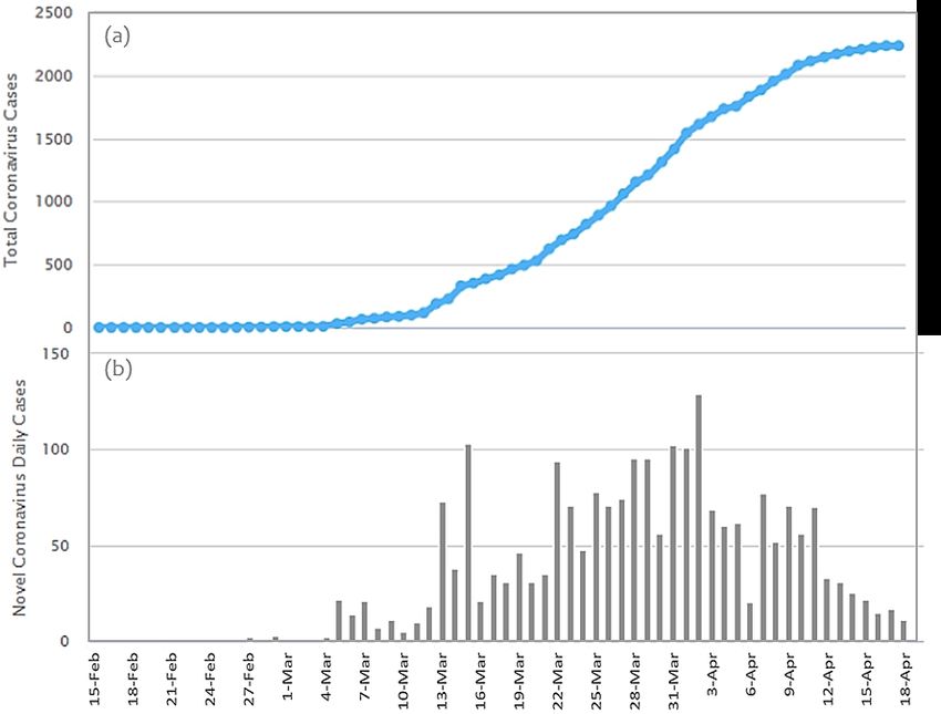
PREPRINT                                                                                               8 of 16

variable for further research. Also, the number of patients in ICU (X7) appears significantly and negatively
correlated with the number of infections (X2) and deaths (X3), implying that the number of patients in
ICU tend to decrease when the number of infections and deaths increases. This observation is rationale
since cases of death are removed from the ICU. On the other hand, the number of patients in ICU (X7) is
significantly and positively correlated with the number of daily infections (X4), implying that the number
of patients entering in ICU tend to increase when the number of daily infections gets bigger. Next, an
interesting observation regards the correlations between the number of tests (X4) and variables X2 and
X3. Although these correlations r(X4,X2) and r(X4,X3) are significant and positive, as expected (implying
that the number of tests appears proportional to the number of infections and deaths), the numerical
values of these coefficients do not appear considerably high (since r(X4,X2), r(X4,X2) < 0.6). Provided that
a perfect positive linearity between the number of tests and infections (or deaths) implies a increasing
awareness of the health system proportionally to the spread of the disease, the considerable high
distance (> 40%) of the correlation coefficients r(X4,X2), r(X4,X2) from the perfect (positive) linearity can
be seen as an aspect of testing ineffectiveness of the health system in Greece. Overall, the correlation
analysis showed that different aspects of the disease in Greece are ruled by non-randomness and
therefore it provided indications that the evolution of the Greek COVID-19 system is driven by sort-term
linear trends. Therefore, a stochastic analysis is further applied for the improvement of the overall
systems’ determination and thus for the better conceptualization of the dynamics ruling the evolution of
COVID-19 in Greece.

4.1. Regression Analysis
The first approach for modeling the evolution of the GOVID-19 infection curve builds on regression
analysis and generally on the curve fitting approach (Walpole et al., 2012), according to which a
parametric curve is fitted to the data of variable X2=f(t) that bests describes its variability through time.
The available types of fitting curves examined in the regression analysis are the linear, quadratic (2nd
order polynomial), cubic (3nd order polynomial), power, and logarithmic. All the available types of fitting
curves can be generally described by the general multivariate linear regression model expressed by the
formula (Walpole et al., 2012):
                           ̂                                      ∑                                     (1),
by considering that each independent variable xi can represent a function of x, namely xi =f(x), as it is
shown in relation (2).
                                             ̂    ∑
                                                                         (2),
     The function f(x) can be either logarithmic f(x)=(log(x))m, or polynomial f(x)=xm, or exponential
f(x)=(exp{x})m, or any other. Within this context, the purpose of the regression analysis is estimating the
parameters bi of model (2) that best fit to the observed data y, so that to minimize the square
differences       ̂ (Walpole et al., 2012), namely:
                               {    ∑    [       ̂]       ∑   [   ∑             ] }                     (3).
     The algorithm estimates the beta coefficients (bi) by using the Least-Squares Linear Regression
(LSLR) method (Walpole et al., 2012), based on the assumption that the differences e in relation (3)
follow the normal distribution N(0, ). In this paper, the time (days since the first infection, variable X1)
are set as the independent variable and each other available variable are set as response variables to the
models. In all cases, the simplest form of regression models that best fits the data is chosen. The
simplicity criterion regards both the number of the used terms                and the polynomial degree m.
That is, the model with the least possible terms and the lowest possible degree m < n-2 (where n is the
number of observations in the data-set) is chosen if it best fits the data. The determination ability of each
model is expressed by the coefficient of determination R2, which is given by the formula (Norusis, 2008;
Walpole et al., 2012):
                                                      ∑       ̂
                                                      ∑       ̅
                                                                                                       (4),
PREPRINT 9 of 16
where are the observed values of the response (independent) variable, ̂ are the estimated values
of the response variable, ̅ is the average of the observed values of the response variable and n is the
number of observations (the length of the variables). The coefficient of determination expresses the
amount of the variability of the response variable is expressed by the model ̂ and ranges within the
interval [0,1], showing perfect determination when equals to one (Norusis, 2008; Walpole et al., 2012).
Another measure of fitting ability is the root mean square deviation or error (RMSD or RMSE),
which calculates the square root of the expected differences between the predicted ( ̂) and the
observed (y) values of the model, according to the formula (Norusis, 2008; Walpole et al., 2012):
√ ̂ =√ ̂ (5),
where E(·) is the function of the expected value. The RMSE represents the square root of the second
sample moment of the regression residuals (Norusis, 2008; Walpole et al., 2012).
A final measure of fitting ability used in the analysis is the relative absolute error (RAE), which
calculates the relative value of the RMSE in accordance with the expected observed values, as it is shown
at the formula (Norusis, 2008; Walpole et al., 2012):
√ ̂ ⁄√ (6),
where E(·) is the function of the expected value. The RAE is often used in machine learning, data mining,
and operations management applications, and represents the analogy of the RMSE relatively to the
expected value of the observed values.
Within this context, Fig.6 shows the results of the regression analysis applied to the (cumulative)
number of infections (dependent variable: X2). As it can be observed, the 3rd order polynomial (cubic)
fitting curve best describes the data of the Greek COVID-19 cumulative infections. The last (very recent)
part of the cubic curve appears convex implying that the number of cumulative infections tends to
saturate.
Fig.6. Available types of fitting curves applied to the cumulative COVID-19 infection curve (variable X2) of Greece. Time-series data
of the variable are shown in dots.
Next, Fig.7 shows the results of the regression analysis applied to the (cumulative) number of
deaths (dependent variable: X4). As it can be observed, similarly to variable X2, the 3rd order polynomial
(cubic) fitting curve best describes the data of the Greek COVID-19 cumulative deaths. The shape of this
curve also implies that the number of cumulative infections tends to saturate.PREPRINT 10 of 16
Fig.7. The available types of fitting curves applied to the cumulative COVID-19 death curve (variable X4) of Greece. Time-series data
of the variable are shown in dots.
Finally, Fig.8 shows the results of the regression analysis applied to the cumulative number of
patients in ICU (dependent variable: cumulative X7). Similarly to variables X2 and X4, the 3rd order
polynomial (cubic) fitting curve best describes the data of (cumulative) variable X7 and the shape of the
curve implies that the number of cumulative ICU patients also tends to saturate.
Fig.8. The available types of fitting curves applied to the cumulative COVID-19 ICU patients (variable: cumulative X7) of Greece.
Time-series data of the variable are shown in dots.
The regression analysis has shown that the best fitting to the cumulative expressions of the
COVID-19 infection (X2), death (X4), and ICU patients (X7) curves in Greece better fit to 3rd order
polynomial (Cubic) than to linear, power, logarithmic, or 2nd order polynomial patterns. As it was
previously observed, the cubic-shape of the fitting curves (which ends up to a convex area representing
the recent past of the time-series) illustrates saturation trends of the COVID-19 evolution in Greece. To
improve the accuracy and the determination ability of the fittings we apply at next a regression analysis
based on the Regression Splines algorithm.
4.2. Regression SplinesPREPRINT 11 of 16
A regression spline is a special piecewise polynomial function defined in parts and is widely used in
interpolation problems requiring smoothing. In particular, for a given partition a=to < t1 < t2 < … < tk-1 <
tn=b of the interval [a,b], a spline is a multi-polynomial function S(t) defined by the union of functions (De
Boor et al., 1978):
[ ] ⋃ [ ] ⋃ ⋃ [ ] ⋃ [ ] ⋃ [ ] (5),
where k is the number of knots t=(to,t1,t2,…,tn) dividing the interval [a,b] into k-1 convex subintervals.
Each function Si(t), i=1,…,n, is a polynomial of low (usually square) degree (sometimes can also be linear)
that is fitter to the corresponding interval [ti-1, ti], i=1,…,n, so that the aggregate spline function to be
continuous and smooth. The spline algorithm is preferable than this of simple regression in cases when
the simple regression generates models of high degree (De Boor et al., 1978). This piecewise approach
yields models of high determination by using low degree polynomial piece-functions. In terms of the
bias-variance trade-off dilemma (Geman et al., 1992), stating that simple (i.e. of low degree) models have
small variance and high bias whereas complex models have small bias and high variance, the spline
algorithm can generate fittings of both low variance and low bias and thus it minimizes the expected loss
expressed by the sum of square bias, variance, and noise.
The major modeling choices for applying splines is, first, the determination of the knot vector
t=(to,t1,t2,…,tn) so that to obtain the smoothest and of best determination spline model, and, secondly,
the selection of the polynomial degree so that the model to be smooth and continuous at the borders of
the sub-intervals. Therefore, this highly effective (in terms of model determination) fitting method is very
sensitive to the selection of the knot vector, which is usually being determined either uniformly, or
arbitrarily, or intuitively, or based on the researchers’ experience (De Boor et al., 1978; Geman et al.,
1992). The more sophisticated knot-selection techniques existing in the literature (Li et al., 2004, 2005)
build on heuristics to determine the knot vector generating the best fitting and smoothening of the
spline model. Within this open debate of knot determination, this paper builds on the recent work of
Tsiotas and Magafas (2020) and introduces a novel approach for the determination of the spline knot
vector, based on complex network analysis. The proposed method is implemented on the COVID-19
infection curve of Greece and is compared with the previously best fitting models applied to variable X2.
4.3. Complex network analysis of time-series
Transforming a time-series to a complex network is a modern approach that became recently popular,
with the emergence of network science in various fields of research (Barabasi, 2016; Tsiotas and
Charakopoulos, 2020). The most popular method to transform a complex network to a time-series is the
visibility graph algorithm, which was proposed by Lacasa et al. (2008) and became dominant due to its
intuitive conceptualization. In particular, the rationale of creating a time-series to a complex network
(visibility graph) builds on considering the time-series as a path of successive mountains of different
height (each representing the value of the time-series at the certain time). In this time-series-based
landscape, an observer standing on a mountain can see (either forward or backwards) as far as no other
mountain obstructs its visibility. In geometric terms, a visibility line can be drawn between two points
(nodes) of the time-series whether no other intermediating node is higher than this pair of points and
obstructs their visibility (Lacasa et al., 2008; Tsiotas and Magafas, 2020). Therefore, two time-series
nodes can enjoy a connection in the associated visibility graph if they are visible through a visibility line
(Lacasa et al., 2008). The visibility algorithm conceptualizes the time-series as a landscape and produces
a visibility graph associated to this landscape (Tsiotas and Charakopoulos, 2020). The associated (to the
time-series) visibility graph is a complex network where complex network analysis can be further applied
(Tsiotas and Charakopoulos, 2020; Tsiotas and Magafas, 2020).
Within this context, by transforming the time-series of the COVID-19 infection curve to a visibility
graph we can study the time-series as a complex network. This allows dividing the visibility graph of the
COVID-19 infection into connective communities based on the modularity optimization algorithm of
Blondel et al. (2008). This algorithm is heuristic and separates a complex network into communities
which are dense within (i.e. links inside the communities are the highest possible) and sparse between
(i.e. links inside the communities are the highest possible) the (Blondel et al., 2008; Fortunato, 2010;
Tsiotas, 2019). Therefore, the most distant nodes within each community can define the knots for
applying the spline algorithm. This complex-network-based definition (i.e. community detection basedPREPRINT 12 of 16
on modularity optimization) of the knot vector offers the missing conceptualization to the splines knots,
defining them as borderline points of connectivity of the modularity-based communities. According to
this approach, the visibility graph of the COVID-19 infection curve is divided to five modularity-based
communities, which correspond to the periods Q1=[ ] ⋃[ ] , Q2=[5,8], Q3=[20,26], Q4=[27,32], and
Q5=[33,43], as it is shown in Fig.9, where positive integers in these intervals are elements of variable X1.
Fig.9. Community detection of the Greek COVID-19 infection visibility graph based on the modularity optimization algorithm of
Blondel et al. (2008). Node size in the network is proportional to node degree.
Consequently, the spline knot vector can be defined by the knots t=(1,4,8,19,26,32,43) in the body of
the time-series COVID-19 infection curve. This partition facilitates to apply the spline regression algorithm
and to compare the determination ability of the spline model with the cubic regression models
previously shown.
5. RESULTS AND DISCUSSION
After the complex-network-based determination of the spline knot vector, the spline regression
algorithm is applied to the COVID-19 infection curve. The results are shown in Table 2, in comparison with
the cubic fittings and with regression splines of randomly selected (3, 4 and 5) knots. As it can be
observed, in all cases (i.e. for the dependent variables X2, X4, and X7), the proposed complex-network
spline models have better determination ability and lower error terms than both the cubic models
resulted by the regression analysis and the randomly calibrated splines. In particular, improvements
caused by the proposed method range between 0.00–0.20% for the multiple correlation coefficients (R),
between 0.10–0.51% for the model determination (R2), between 0.37–41.32% for the root mean square
error (RMSE), and 0.25–34.19% for the relative absolute error (RAE). These improvements are
considerable even in the cases of R and R2, given the already good fitting performance of the cubic and
the randomly calibrated spline models.
Table 2
Comparison between the polynomial cubic and regression splines fitting curves
Model R R2 RMSE* RAE**
Dependent Variable: Infections (X2)
Cubic 0.998 0.996 2.229 4.182%
Regression Splines with 3 random knots 0.999 0.998 1.805 3.798%
Regression Splines with 4 random knots 0.999 0.998 1.621 3.277%PREPRINT 13 of 16
Model R R2 RMSE* RAE**
Regression Splines with 5 random knots 0.999 0.998 1.420 2.986%
Complex-Network Regression Splines 1.000 1.000 1.308 2.752%
Dependent Variable: Deaths (X4)
Cubic 0.995 0.990 2.423 4.981%
Regression Splines with 3 random knots 0.995 0.990 2.584 5.013%
Regression Splines with 4 random knots 0.995 0.990 2.423 4.798%
Regression Splines with 5 random knots 0.995 0.990 2.410 4.732%
Complex-Network Regression Splines 0.995 0.991 2.401 4.720%
Dependent Variable: ICU patients (X7)
Cubic 0.987 0.974 6.300 12.659%
Regression Splines with 3 random knots 0.987 0.974 6.287 12.648%
Regression Splines with 4 random knots 0.988 0.976 6.186 12.114%
Regression Splines with 5 random knots 0.989 0.979 6.204 12.007%
Complex-Network Regression Splines 0.989 0.979 6.119 11.731%
*
. Relative mean square error
**
. Relative absolute error
According to these results, the proposed complex-network-based splines regression method
outperforms in fitting determination both the cubic regression and the randomly-calibrated splines
regression models, which are also models of high accuracy. In conceptual terms, this outperformance
may be related with the immanent property of complex network analysis to model and manage
problems of complexity and thus to provide better insights in the study complex systems, as in the case
of the COVID-19 temporal spread. Despite the restriction in data availability, improvements (mainly in
error terms) achieved by the proposed model are not negligible and highlight the direction of using
hybrid or combined methodologies for dealing with cases of insufficient information. Moreover, the
overall approach highlights the utility of multidisciplinary and synthetic modeling for dealing with
complexity in epidemiology, which by default deals with complex socio-economic systems of humanity.
Given the small data availability, this improvement in the modeling determination is a promising
advantage of the proposed method, which allows building on a quantitative consideration of the spline
knot vector instead of an intuitive one. Besides, the utility and effectiveness of the proposed
methodology should be evaluated in conjunction with the good performance of the spline results against
multi-collinearity (Norusis, 2008; Walpole et al., 2012), which emerges in simple regression modeling due
to the consideration of additional parameters.
Overall, the two major advantages of the proposed method concern the better stability and
capability of forecasting, since the total behavior of the proposed model appears less noisy, while it
reduces the errors of determination due to the modelers’ choices. This conclusion can also be supported
by the variance minimization of the expected error terms, which provides strong indications of the
system’s reliability.
6. CONCLUSIONS
Accurate forecasting is a major task in epidemiology that becomes very important today in the global
emergence that the COVID-19 pandemic has caused. Due to the low availability of data, the worldwide
conceptualization of the new pandemic is currently constraint and still emerging. Within the context of
information lack, methods contributing to more accurate forecasting on early datasets are welcomed
and pertinent for the ongoing fight against the disease. This paper proposed a novel method for
modeling and forecasting in epidemiology based on complex network analysis and spline regression
algorithm. Based on data of the COVID-19 temporal spread in Greece, the proposed method converted aPREPRINT 14 of 16
time-series to an associated visibility graph and then it divided the graph into connected communities
that defined the spline knot vector. This approach provided a complex-network definition of the spline
knots, the definition of which is currently either intuitive or heuristic, and it assigned a conceptualization
to the knots based on network connectivity.
Within this context, the proposed method was applied to different aspects of the COVID-19
temporal spread in Greece (the cumulative number of infections, deaths, and ICU patients) and found to
outperform the regression cubic models, which had the highest determination amongst the available
simple regression models. In methodological terms, the overall approach advances the spline regression
algorithm, which is currently restricted to the not-well defined determination of knots, whereas, in
practical implementation, the proposed methodology offers an active method for modeling and
forecasting the pandemic, capable in removing the disconnected past data from the time-series
structure. In terms of health policy, this paper provides a modeling and forecasting tool facilitating
decision making and resource management in epidemiology, which can contribute in the ongoing fight
against the pandemic of COVID-19.
REFERENCES
Ahmed, S. F., Quadeer, A. A., & McKay, M. R. (2020). Preliminary identification of potential vaccine targets for the
COVID-19 coronavirus (SARS-CoV-2) based on SARS-CoV immunological studies. Viruses, 12(3), 254.
Anastassopoulou, C., Russo, L., Tsakris, A., Siettos, C., (2020) “Data-based analysis, modeling and forecasting of the
COVID-19 outbreak”, PLoS ONE, 15(3), e0230405.
Bai, Y., Yao, L., Wei, T., Tian, F., Jin, D. Y., Chen, L., & Wang, M. (2020). Presumed asymptomatic carrier transmission
of COVID-19. Jama, 323(14), 1406-1407.
Barabási, A. L. (2016). Network science. Cambridge university press.
Blondel, V., Guillaume, J.-L., Lambiotte, R., Lefebvre, E., (2008) “Fast unfolding of communities in large networks”,
Journal of Statistical Mechanics, 10, P10008. https://doi.org/10.1088/1742-5468/2008/10/P10008.
De Boor, C., De Boor, C., Mathématicien, E. U., De Boor, C., & De Boor, C. (1978). A practical guide to splines (Vol. 27,
p. 325). New York: springer-verlag.
Fang, Y., Zhang, H., Xie, J., Lin, M., Ying, L., Pang, P., & Ji, W. (2020). Sensitivity of chest CT for COVID-19: comparison
to RT-PCR. Radiology, 200432.
Fong, S.j., Li, G., Dey, N., Crespo, R. G., Herrera-Viedma, E., (2020) “Finding an Accurate Early Forecasting Model
from Small Dataset: A Case of 2019-nCoV Novel Coronavirus Outbreak”, International Journal of Interactive
Multimedia and Artificial Intelligence, 6(1), pp.132-40.
Fortunato, S., (2010) “Community detection in graphs”, Physics Reports, 486, pp.75–174.
https://doi.org/10.1016/j.physrep.2009.11.002.
Geman, S., Bienenstock, E., & Doursat, R. (1992). Neural networks and the bias/variance dilemma. Neural
computation, 4(1), 1-58.
Giuliani, D., Dickson, M.-M., Espa, G., and Santi, F., (2020) “Modelling and Predicting the Spatio - Temporal Spread
of Coronavirus Disease 2019 (COVID -19) in Italy”, (10.2139/ssrn.3559569).
Heymann, D. L., & Shindo, N. (2020). COVID-19: what is next for public health?. The Lancet, 395(10224), 542-545.
Lacasa, L., Luque, B. , Ballesteros, F., Luque, J., Nuno, J.C., (2008) “From time-series to complex networks: The
visibility graph”, Proceedings of the National Academy of Sciences, 105(13), pp.4972–4975.
Lescure, F. X., Bouadma, L., Nguyen, D., Parisey, M., Wicky, P. H., Behillil, S., ... & Enouf, V. (2020). Clinical and
virological data of the first cases of COVID-19 in Europe: a case series. The Lancet Infectious Diseases.
Li, W., Xu, S., Zhao, G., & Goh, L. P. (2004). A heuristic knot placement algorithm for B-spline curve approximation.
Computer-Aided Design and Applications, 1(1-4), 727-732.
Li, W., Xu, S., Zhao, G., & Goh, L. P. (2005). Adaptive knot placement in B-spline curve approximation. Computer-Aided
Design, 37(8), 791-797.
Liu, W., Zhang, Q., Chen, J., Xiang, R., Song, H., Shu, S., ... & Wu, P. (2020). Detection of Covid-19 in children in early
January 2020 in Wuhan, China. New England Journal of Medicine, 382(14), 1370-1371.
Livingston, E., Bucher, K., (2020) “Coronavirus disease 2019 (COVID-19) in Italy”, Jama.
Lurie, N., Saville, M., Hatchett, R., & Halton, J. (2020). Developing Covid-19 vaccines at pandemic speed. New England
Journal of Medicine.PREPRINT 15 of 16
Mahase, E., (2020) “COVID-19: UK starts social distancing after new model points to 260 000 potential deaths”, BMJ,
368:m1089.
Ministry of Health of Greece – MOHG (2020), “Press Releases”, available at the URL:
https://www.moh.gov.gr/articles/ministry/grafeio-typoy/press-releases [accessed: 30/4/20].
National Public Health Organization of Greece – NPHOG (2020) “New coronavirus Covid-19 - Instructions”, available
at the URL: https://eody.gov.gr/neos-koronaios-covid-19 [accessed: 26/4/2020].
Norusis, M., (2008) SPSS 16.0 advanced statistical procedures companion, Prentice Hall Press.
Our World in Data, (2020) “Total confirmed COVID-19 deaths per million people”, available at the URL:
https://ourworldindata.org/grapher/total-covid-deaths-per-million?year=2020-04-26 [accessed: 26/4/2020].
Petropoulos, F., Makridakis, S., (2020) “Forecasting the novel coronavirus COVID-19”, PLoS ONE, 15(3), e0231236.
Qiu, H., Wu, J., Hong, L., Luo, Y., Song, Q., & Chen, D. (2020). Clinical and epidemiological features of 36 children with
coronavirus disease 2019 (COVID-19) in Zhejiang, China: an observational cohort study. The Lancet Infectious
Diseases.
Remuzzi, A., Remuzzi, G., (2020) “COVID-19 and Italy: what next?”, The Lancet.
Roser, M., Ritchie, H., (2020) “Coronavirus Disease (COVID-19)" available at the URL:
https://ourworldindata.org/coronavirus-data [accessed: 10/4/20]
Sarkodie, S.A., Owusu, P.A., (2020) “Investigating the cases of novel coronavirus disease (COVID-19) in China using
dynamic statistical techniques”, Heliyon, 6(4), e03747.
Shi, H., Han, X., Jiang, N., Cao, Y., Alwalid, O., Gu, J., ... & Zheng, C. (2020). Radiological findings from 81 patients with
COVID-19 pneumonia in Wuhan, China: a descriptive study. The Lancet Infectious Diseases.
Tan, L., Wang, Q., Zhang, D., Ding, J., Huang, Q., Tang, Y. Q., ... & Miao, H. (2020). Lymphopenia predicts disease
severity of COVID-19: a descriptive and predictive study. Signal transduction and targeted therapy, 5(1), 1-3.
Tsiotas, D., Charakopoulos, A., (2020) “VisExpA: Visibility expansion algorithm in the topology of complex
networks”, Software X, 11, 100379.
Tsiotas, D., Magafas, L., (2020) “The effect of anti-COVID-19 policies to the evolution of the disease: A complex
network analysis to the successful case of Greece”, arXiv.2004.06536.
Walpole, R. E., Myers, R. H., Myers, S. L., Ye, K., (2012) Probability & Statistics for Engineers & Scientists, ninth ed., New
York, Prentice Hall Publications.
Worldometers, (2020) “COVID-19 coronavirus pandemic”, available at the URL: www.worldometers.info/coronavirus
[accessed: 20/4/2020].
Xu, B., Gutierrez, B., Mekaru, S. et al. (2020) “Epidemiological data from the COVID-19 outbreak, real-time case
information”, Sci Data, 7(106) (doi:10.1038/s41597-020-0448-0).
Xu, B., Gutierrez, B., Mekaru, S., Sewalk, K., Goodwin, L., Loskill, A., ... , Zarebski, A. E., (2020b) “Epidemiological data
from the COVID-19 outbreak, real-time case information”, Scientific Data, 7(1), pp.1-6.
Xu, Z., Shi, L., Wang, Y., Zhang, J., Huang, L., Zhang, C., ... & Tai, Y. (2020a). Pathological findings of COVID-19
associated with acute respiratory distress syndrome. The Lancet respiratory medicine, 8(4), 420-422.
Ye, Z., Zhang, Y., Wang, Y., Huang, Z., & Song, B. (2020). Chest CT manifestations of new coronavirus disease 2019
(COVID-19): a pictorial review. European Radiology, 1-9.
APPENDIX A
Table Α1
The COVID-19 variables participating in the analysis(a)
Date Day Infections Daily Infections Deaths Daily Deaths Daily Recovered ICU Tests
(X1) (X2) (X3) (X4) (X5) (X6) (X7) (X8)
26-Feb-20 1 1 1 0 0 0 0 0
27-Feb-20 2 3 2 0 0 0 0 0
28-Feb-20 3 4 1 0 0 0 0 0
29-Feb-20 4 7 3 0 0 0 0 0
1-Mar-20 5 9 0 0 0 0 0 0
2-Mar-20 6 9 0 0 0 0 0 0
3-Mar-20 7 9 0 0 0 0 0 270
4-Mar-20 8 11 2 0 0 0 1 0
5-Mar-20 9 31 22 0 0 0 0 0
6-Mar-20 10 46 14 0 0 0 1 0PREPRINT 16 of 16
Date Day Infections Daily Infections Deaths Daily Deaths Daily Recovered ICU Tests
(X1) (X2) (X3) (X4) (X5) (X6) (X7) (X8)
7-Mar-20 11 66 21 0 0 0 0 0
8-Mar-20 12 73 7 0 0 0 0 0
9-Mar-20 13 84 11 0 0 0 1 0
10-Mar-20 14 89 5 0 0 0 1 0
11-Mar-20 15 99 10 0 0 0 2 0
12-Mar-20 16 117 18 0 1 2 0 1910
13-Mar-20 17 190 73 1 0 0 3 520
14-Mar-20 18 228 38 1 2 6 0 700
15-Mar-20 19 331 103 3 1 2 2 0
16-Mar-20 20 352 21 4 0 0 5 920
17-Mar-20 21 387 35 4 1 4 2 580
18-Mar-20 22 418 31 5 0 0 6 1100
19-Mar-20 23 464 46 5 1 5 5 300
20-Mar-20 24 495 31 6 3 0 4 872
21-Mar-20 25 530 35 9 4 0 3 658
22-Mar-20 26 624 94 13 2 0 9 176
23-Mar-20 27 695 71 15 2 10 4 638
24-Mar-20 28 743 48 17 3 3 5 427
25-Mar-20 29 821 78 20 2 4 5 1424
26-Mar-20 30 892 71 22 4 6 2 0
27-Mar-20 31 966 74 26 2 10 9 2982
28-Mar-20 32 1061 95 28 4 0 1 886
29-Mar-20 33 1156 95 32 6 0 -2 788
30-Mar-20 34 1212 56 38 5 0 3 810
31-Mar-20 35 1314 102 43 6 0 13 771
1-Apr-20 36 1415 101 49 1 0 5 618
2-Apr-20 37 1544 129 50 3 9 1 1494
3-Apr-20 38 1613 69 53 6 17 1 3593
4-Apr-20 39 1673 60 59 9 0 0 896
5-Apr-20 40 1735 62 68 5 0 1 2120
6-Apr-20 41 1755 20 73 6 191 -3 740
7-Apr-20 42 1832 77 79 2 0 0 2391
8-Apr-20 43 1884 52 81 2 0 -6 3944
9-Apr-20 44 1955 71 83 3 0 -5 1106
10-Apr-20 45 2009 56 86 4 0 -2 1798
11-Apr-20 46 2081 70 90 3 0 -2 1912
12-Apr-20 47 2114 33 93 5 0 1 4917
13-Apr-20 48 2145 31 98 1 0 -3 1156
14-Apr-20 49 2170 25 99 2 0 3 5381
15-Apr-20 50 2192 22 101 1 0 -4 1973
16-Apr-20 51 2207 15 102 3 0 -3 0
17-Apr-20 52 2224 17 105 3 0 2 0
18-Apr-20 53 2235 11 108 2 0 -4 2519
19-Apr-20 54 2235 0 110 3 0 -4 0
Sum 2235 2235 113 113 269 69 53290
*. All data were daily extracted from National Public Health Organization of Greece (2020)You can also read