Evidence of Hierarchy in the Drainage Basins Size Distribution of Greece Derived from ASTER GDEM-v2 Data - MDPI
←
→
Page content transcription
If your browser does not render page correctly, please read the page content below
applied
           sciences
Article
Evidence of Hierarchy in the Drainage Basins Size
Distribution of Greece Derived from ASTER
GDEM-v2 Data
Filippos Vallianatos 1,2, * and Maria Kouli 2
 1    School of Sciences, Faculty of Geology and Geoenvironment, Department of Geophysics—Geothermics,
      National and Kapodistrian University of Athens, University Campus, Panepistmiopolis,
      GR 15784 Athens, Greece
 2    UNESCO Chair on Solid Earth Physics and Geohazards Risk Reduction, Hellenic Mediterranean University,
      Crete, GR 73133 Chania, Greece; mkouli@chania.teicrete.gr
 *    Correspondence: fvallian@geol.uoa.gr; Tel.: +30-210-727-4360

 Received: 31 October 2019; Accepted: 20 December 2019; Published: 28 December 2019

 Abstract: The drainage basins of Greece are analyzed in terms of hierarchy and discussed in view
 of Tsallis Entropy. This concept has been successfully used in a variety of complex systems, where
 fractality, memory and long-range interactions are dominant. The analysis indicates that the statistical
 distribution of drainage basins’ area in Greece, presents a hierarchical pattern that can be viewed
 within the frame of non-extensive statistical physics. Our work was based on the analysis of the
 ASTER GDEM v2 Digital Elevation Model of Greece, which offers a 30 m resolution, creating an
 accurate drainage basins’ database. Analyzing the drainage size (e.g., drainage basin area)-frequency
 distribution we discuss the connection of the observed power law exponents with the Tsallis entropic
 parameters, demonstrating the hierarchy observed in drainage areas for the set created for all over
 Greece and the subsets of drainages in the internal and external Hellenides that are the main tectonic
 structures in Greece. Furthermore, we discuss in terms of Tsallis entropy, the hierarchical patterns
 observed when the drainages are classified according to their relief or the Topographic Position Index
 (TPI). The deviation of distribution from power law for large drainages area is discussed.

 Keywords: drainage basins; geomorphology; Tsallis entropy; active tectonics; Greece; ASTER GDEM

1. Introduction
      Nature displays power laws in frequency distributions of diverse phenomena [1,2]. Scaling theories
as expressed by power laws play an important role in quantification of scale invariance in Earth systems.
From the classical study of earthquakes to complex geosystems analysis, the appearance of power
law behavior has been seen as the signature of hierarchy. The present study is part of a systematic
attempt to examine the dynamics of earth system by implementing the generalized non-extensive
statistical physics (NESP) formalism. Investigation of the scaling properties of a geomorphological
system strongly suggests the development of complex systems associated with their dynamics [3,4].
To understand this scientific challenge, we apply modern statistical physics approaches to understand
the dynamics of geomorphological effects.
      Analyses of power-law behavior in earth systems frequently invoke self-organized criticality
(SOC) [1,5] to explain evolution towards the observed hierarchical structure. Geomorphologists
seek to understand landscapes evolution, landform history and dynamics and to evaluate changes
through a combination of field observations, physical experiments and numerical modeling. Landscape
dynamics is governed mainly by slope and fluvial processes both operating in a drainage network [6],
resulting after combining a large-amplitude climatic fluctuations along with tectonic uplift/subsidence

Appl. Sci. 2020, 10, 248; doi:10.3390/app10010248                              www.mdpi.com/journal/applsci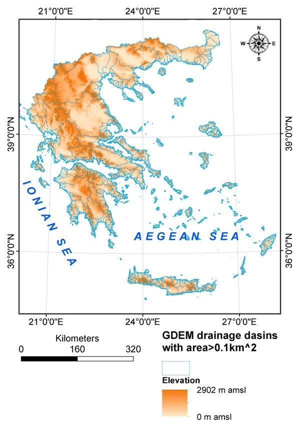
Appl. Sci. 2020, 10, 248                                                                            2 of 18

activity. As a result the complex interaction between earth’s surface and tectonic processes plays a
key role in geomorphological evolution [7]. Tectonic activity generates complex relief that controls
surface processes such as erosion patterns, drainage network development, sedimentary basin growth,
and local climate [8–12]. Moreover, erosion, transport and sedimentation induce large mass transfer
that changes the dynamical equilibrium of orogenic wedges and trigger mechanical actions [8,13].
The continuous evolution of the aforementioned processes, in a dynamical non-linear feedback indicates
a system in a dynamical non-equilibrium stage where long-range interactions and memory effects
are dominant.
      In this context, geomorphologists have studied the evolution of drainages in time and found it to
be driven by local conditions due to erosion, natural damming, tectonic motion, as well as volcanic
activity [14–16]. A drainage basin is an area of land that drains all the streams and rainfall to a
common outlet such as the outflow of a reservoir, mouth of a bay, or any point along a stream channel.
Drainage basins as conceptual or physical entities are used in water management [17,18], landsliding
processes control [19] and flood control [20,21].
      According to Strahler and Strahler [22], the development of a drainage system (i.e., a stream
network and its drainage basin) can be described as follows: Initially, the stream is established on a
land surface dominated by landforms of tectonic activity. In a next stage, the channels are deepening
due to gradation resulting in steep gorges while the stream tributaries extend into the land carrying
out a drainage basin and transforming the landscape into a fluvial landform system. Moreover, after
reaching a state of balance (i.e., the supply of load becomes equal to the capacity of the stream to
transport it), the stream continues to cut laterally its banks resulting in an extension of the drainage
basin. The quantification of drainage geometry aims to study the underlying organization and to
offer an insight to the physical processes controlling their evolution. Cumulative area distribution
is a geomorphologic measure that characterizes the drainage basin hydrology and is widely used
by geomorphologists to characterize the possible existence of their scale invariant structure and the
scaling properties of the drainage area [23–26].
      Recently, non-extensive statistical physics [27,28] have been becoming a valuable framework for
interpreting geo-environmental complex systems [29–35]. Drainages obtain long range interaction,
multi-fractality and present a memory of the geological and physical processes involved in their
evolution. Since memory and fractality are two of the key components of any geophysical
process [36–38] we can use a current generalization of Boltzmann-Gibbs (BG) statistical physics,
referred as non-extensive statistical physics (NESP) [27,28,36] to justify the hierarchy pattern presented
in drainage area distribution.
      The advantage of considering the Tsallis distribution [28] is that, based on the fundamental
principle of Tsallis entropy, scaling laws observed in phenomena that present fractality, long range
interaction and memory effects [27,28] could be interpreted. We note that recent applications to solid
earth physics (in regional or planetary scale) [31–33,37] and to natural hazards [29,30,38] supports the
applicability of non-extensive statistical physics in complex geosystems. To our knowledge, this is the
first time that Tsallis entropy is used to express and interpret the drainage basins area distribution,
within an effort to present scaling laws as extracted from first principles and not in an empirical basis.
Scaling theories play an important role in quantification of scale invariance in geosystems, since the
appearance of power-law behavior has been seen as the signature of scale invariance.
      Our motivation is to suggest a new view of scaling laws observed in drainage basins of Greece
in terms of Tsallis entropy. A connection between the observed power law exponent and the Tsallis
entropic parameter is suggested. To demonstrate the hierarchy observed in drainage area statistical
pattern, data sets for all drainages all over Greece, along with subsets of drainages in the internal
and external Hellinides, that are the main tectonic structures in Greece, are constructed. Since the
topographic relief is a crucial parameter in drainages formation, we classify them according to the
mean value of the Topographic Position Index (TPI) and the mean elevation. Finally, the observed
hierarchy within each one of the sub-datasets, is interpreted according to non extensive statistical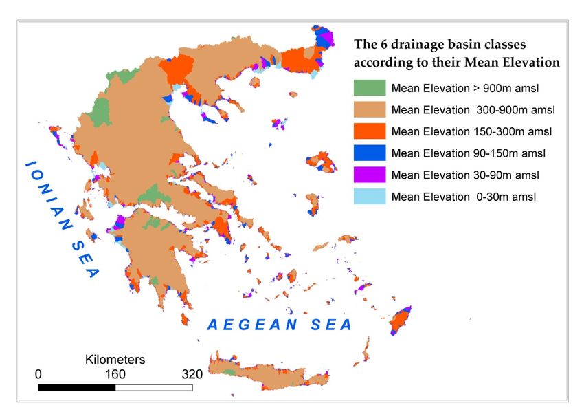
Appl. Sci. 2020, 10, 248                                                                              3 of 18

physics. We clarify that the zonation used is the external input in our analysis, as introduced by
geotectonic and geomorphological critiria. We note that the selection of TPI and of mean elevation
is based on their simplicity as geomorphological measures that control a number of phenomena
(e.g., erosion).
      The remaining of this presentation is organized as follows. A procedure of data extraction
using Advanced Spaceborne Thermal Emission and Reflection Radiometer (ASTER) Global Digital
Elevation Model Version 2 (GDEM V2), images is presented in Section 2. A brief presentation of the
NESP formalism will be given in Section 3, followed by a presentation of the hierarchical drainage
basin analysis applied power law formulation and along with NESP expressions. The analysis as
presented in Section 4, will focus on the drainage data set of Greece along with the subsets created
by the classification of drainages in the geotectonic frame of internal or external Hellenides or using
classifications based on topographic criteria as that of mean elevation or the mean Topographic
Position Index (TPI). Section 5 is devoted to the discussion of the results and to the presentation of a
possible origin of the deviation from power law observed in a number of cases for large drainage area.
Finally, it shall be demonstrated that drainage systems are sub-additive systems with significant long
range interaction where non-extensive statistical physics could be used to understand the observed
hierarchical processes.

2. Drainage Basins Extraction
     It is obvious that drainage basins statistical characterization is critical for understanding the
geomorphic processes.
     During the last decades, geographical information systems (GIS) coupled with digital elevation
models (DEMs) have been widely used for the automatical extraction of drainage networks and
drainage basins as well as for landforms classification [39,40]. In the present work, ASTER GDEM v2,
is used as downloaded from the LP DAAC at one arc sec resolution (30 m) [41]. In comparison with
other free DEMs, Aster GDEM has lower RMS errors in mountainous areas [42,43] and since Greece is
such an area we decided to use it for the watersheds extraction. Aster GDEM was clipped to the extent
of the study area of Greece and re-projected to the Hellenic Geodetic Reference System ‘87 (HGRS’87).
Using ArcHydro, an extension of ArcGIS software, we were capable to efficiently delineate the drainage
basins of Greece. The procedure used is as follows: firstly, the cells with elevation values abnormally
low or high in comparison to their neighboring cells (known as sinks or spikes respectively) were
removed. After the removal of the erroneous data, a new, hydrologically corrected (i.e., free of sinks
and spikes), digital elevation model, was obtained [44]. After that, a flow direction computation using
the commonly used D8 algorithm [45] was applied. D8 flow direction is an integer raster whose values
range from 1 to 255 providing 8 different directions. It is then analyzed to find all sets of connected cells
that belong to the same drainage basin. The drainage basins are delineated within the analysis window
by identifying ridge lines. The drainage basins of the Greek territory were extracted in the form of a
raster layer which was later converted to a vector polygonal one, containing a few thousands of basins.
     From these basins only that with an area greater than 0.1 km2 (Figure 1) were selected for further
analysis based on visual comparison with the national drainage basins dataset. For the area distribution
analysis, the final drainage basin dataset was extracted into several layers (sub-datasets) according to
different attributes and spatial characteristics such as, the geotectonic environment, the mean elevation
value, and the mean topographic position index using the “select by attributes” and “select by location”
functions of ArcGIS software.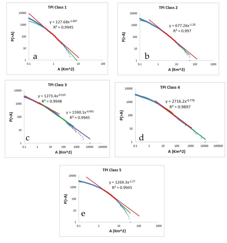
Appl. Sci. 2020, 10, 248                                                                                              4 of 18
Appl. Sci. 2019, 9, x FOR PEER REVIEW                                                                                4 of 17

               Figure 1.
               Figure    The ASTER
                      1. The ASTER GDEM
                                   GDEM of
                                        of Greece
                                           Greece with
                                                  with drainage
                                                       drainage basins
                                                                basins polygonal
                                                                       polygonal data
                                                                                 data overlay.
                                                                                      overlay.

3. The Principles of Non-Extensive Statistical Physics as Applied in Drainage Systems
3. The Principles of Non-Extensive Statistical Physics as Applied in Drainage Systems
      A number of earth physics effects in different spatial and temporal scales, which includes rock
      A number of earth physics effects in different spatial and temporal scales, which includes rock and
and material properties, natural hazards, earthquake mechanics, plate tectonics, geomagnetic reversals
material properties, natural hazards, earthquake mechanics, plate tectonics, geomagnetic reversals and
and geological faults, have been interpreted in terms of the non-extensive statistical mechanics (NESP)
geological faults, have been interpreted in terms of the non-extensive statistical mechanics (NESP) view
view [36]. Here we recapitulate the main principles of NESP in which a cornerstone is the introduction
[36]. Here we recapitulate the main principles of NESP in which a cornerstone is the introduction of the
of the non-extensive Tsallis entropy Sq [28] in terms of the probability distribution p(A) of a fundamental
non-extensive Tsallis entropy Sq [28] in terms of the probability distribution p(A) of a fundamental
geometric parameter, A that in our case could be the watershed area A:
geometric parameter, A that in our case could be the watershed area A:
                                                      − ∑ pq ((A)
                                                        P
                                                    1−         A)
                                           Sq = k B                                                   (1)(1)
                                                        q−− 11
 where kkBB is
where          Boltzmann’s constant.
            is Boltzmann’s     constant. The
                                           The index  q is
                                                index q is the
                                                           the degree
                                                               degree of of non-additivity.
                                                                            non-additivity. In In the
                                                                                                  the limit
                                                                                                       limit q→1,
                                                                                                              q→1, Sq→S
                                                                                                                     Sq→S11
 and  the  approach     reduced   to  the  well-known   Boltzmann-Gibbs        (BG)   entropy,
and the approach reduced to the well-known Boltzmann-Gibbs (BG) entropy, with which the Tsallis  with   which   the  Tsallis
entropy shares many common properties [28]. However, simple additivity is violated, because for
 entropy   shares    many   common      properties  [28]. However,     simple   additivity   is violated,   because    for aa
 system composed
system    composed of   of two
                           two statistically
                                statistically independent
                                               independent systems,
                                                              systems, U  UAA and
                                                                              and UUBB,, the
                                                                                         the Tsallis
                                                                                             Tsallis entropy
                                                                                                      entropy satisfies:
                                                                                                                 satisfies:
                                                                  1−q
                          S (U + U ) = S (U ) + S (U ) +                1S− (U
                                                                             q )S (U )
                            Sq (UA + UB ) = Sq (UA ) + Sq (UB )k+             Sq (UA )Sq (UB )
                                                                          kB
      The last term on the right hand side of this equation describes the interaction between the two
      The
 systems andlast is
                  term
                    the on  the of
                        origin  right   hand side ofThe
                                   non-additivity.    thisindex
                                                            equation   describes
                                                                  q accounts    for the
                                                                                    the interaction     between the two
                                                                                          memory, multifractality       and
systems
 long-range interaction between the elements (drainages) of the analyzed set, and for q < 1, q = 1 and
           and   is the origin  of non-additivity.   The   index  q accounts    for  the  memory,    multifractality    and
long-range     interaction
 q > 1 respectively          between
                       correspond        the elements (drainages)
                                    to super-additivity,    additivityofand
                                                                         thesub-additivity.
                                                                              analyzed set, and Thisfor   q  1 respectively
qprinciple             correspond    to super-additivity,
             of non-extensive statistical mechanics.        additivity  and  sub-additivity.    This is  the fundamental
principle   of non-extensive
      In order                   statistical
                   to estimate the   expected mechanics.
                                                 probability distribution p(A) of the drainage area A, in terms
of NESP, we maximized the non-extensive entropy under the appropriate constraints, using the
Lagrange-multipliers method with the Lagrangian [28,34,37]: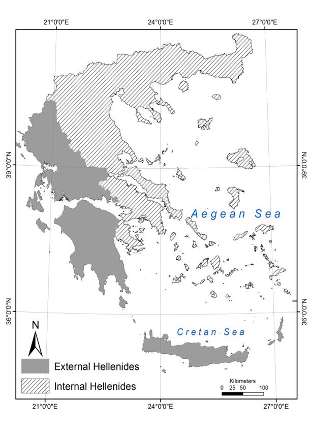
Appl. Sci. 2020, 10, 248                                                                                                      5 of 18

    In order to estimate the expected probability distribution p(A) of the drainage area A, in terms
of NESP, we maximized the non-extensive entropy under the appropriate constraints, using the
Lagrange-multipliers method with the Lagrangian [28,34,37]:
                     Z     ∞                              Z       ∞                          Z       ∞
           Lq = −              pq (A) lnq p(A)dA − λo (               p(A)dA − 1) − λ1 (                 APq (A)dA − hAiq )
                       0                                      0                                  0

      The first constraint used refers to the normalization condition that reads as:
                                              Z ∞
                                                  p(A)dA = 1
                                                     0

Introducing the generalized expectation value (q-expectation value), q which is defined as:

                                                                      Z∞
                                              Aq = hAiq =                  APq (A)dA
                                                                      0

where the escort probability is given in [28] as:

                                                                          pq(A)
                                                Pq (A) = R ∞
                                                                  0
                                                                          pq (A)dA

the extremization of Sq with the above constraints yields to the probability distribution of p(A) as [34]:
                                                          "                       !#    1
                                                              1−q A                    1−q
                                             p ( A ) = Cq 1 −                                                                    (2)
                                                              2 − q Aq

where Cq is a normalization coefficient. We recall that the Q-exponential function introduced in NESP
by Tsallis (2009) is defined as [28]:
                                      (
                                          [1 + (1 − Q)X]1/(1 − Q) if (1 + (1 − Q) X ≥ 0)
                      expQ (X) =
                                             0                    if (1 + (1 − Q) X < 0)

     The normalized cumulative number of drainage with area greater than A can be obtained by
integrating the probability density function p(A) as:

                                                                     !# q−2
                                                N(> A)
                                                        "        !
                                                            q − 1 A q−1
                                       P(> A) =        = 1+                                                                      (3)
                                                  N0        2 − q Aq

where N(>A) is the number of drainages with area larger than A. In the latter expression, if we define
q = 2 − Q1 , this leads to:

                                                              !!          "                  !#−      1
                                                     A                              A                Q−1
                                   P(> A) = expQ   −                  = 1 + (Q − 1)                        ,                     (4)
                                                     Aq                             Aq

having a typical Q-exponential form.
     In the frame of non extensive statistical mechanics approach for drainage with a quite large
area where                                          !
                                                 A
                                         (Q − 1)      >> 1
                                                 Aq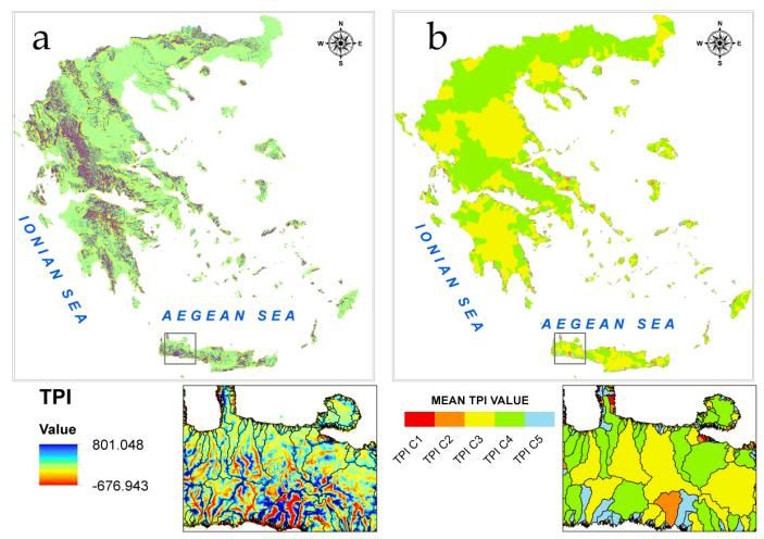
Appl. Sci. 2020, 10, 248 6 of 18
Equation (4) leads to a power law description of the cumulative distribution function
!− 2−q
A q−1
P(> A) C ∼ A−β
Aq
with an exponent
2−q 1
β= = (5)
q−1 Q−1
in agreement with the power law extensively used to describe hierarchical drainage systems [23,25,26,46,47].
4. Hierarchical Drainage Basins Analysis
Here the drainages of Greece were selected and analyzed according to their tectonic regime,
mean elevation value and mean value of Topography Position Index (TPI). In terms of geotectonics, a
distinction between the non-metamorphic External Hellenides of western Greece on the one hand,
characterized by Triassic-Cenozoic sedimentary sequences, and the Internal Hellenides of eastern
Greece on the other, with metamorphic zones of pre-Alpine formations (Figure 2) is used, in order to see
the watershed distribution pattern in this two main geotectonic units that form Greece. The External
Hellenides mainly consist of Meso- and Cenozoic sedimentary rocks deposited in a series of platforms
(Pre-Apulian and Gavrovo zones) and deep basins (Ionian and Pindos zones) that formed the eastern
rifted margin of the Apulian plate, bordering towards the east the Pindos Ocean [48–50]. These units
were developed during Tertiary times following the closure of the Pindos Ocean and the consequent
continent–continent collision between the Apulian and Pelagonian micro-continents to the east [51,52].
This process induced the inversion of Mesozoic basins in the northern margin of Apulia as well as the
formation of a series of thrust sheets comprising the External Hellenides thrust belt ([48] and references
therein). To search the possible connection of drainages hierarchy with the geotectonic environment as
indicated in a number of previous works [21,23,24,46,47] we select to search the drainage distribution
in the two drainage subsets defined by the two main tectonic patterns of Greece.
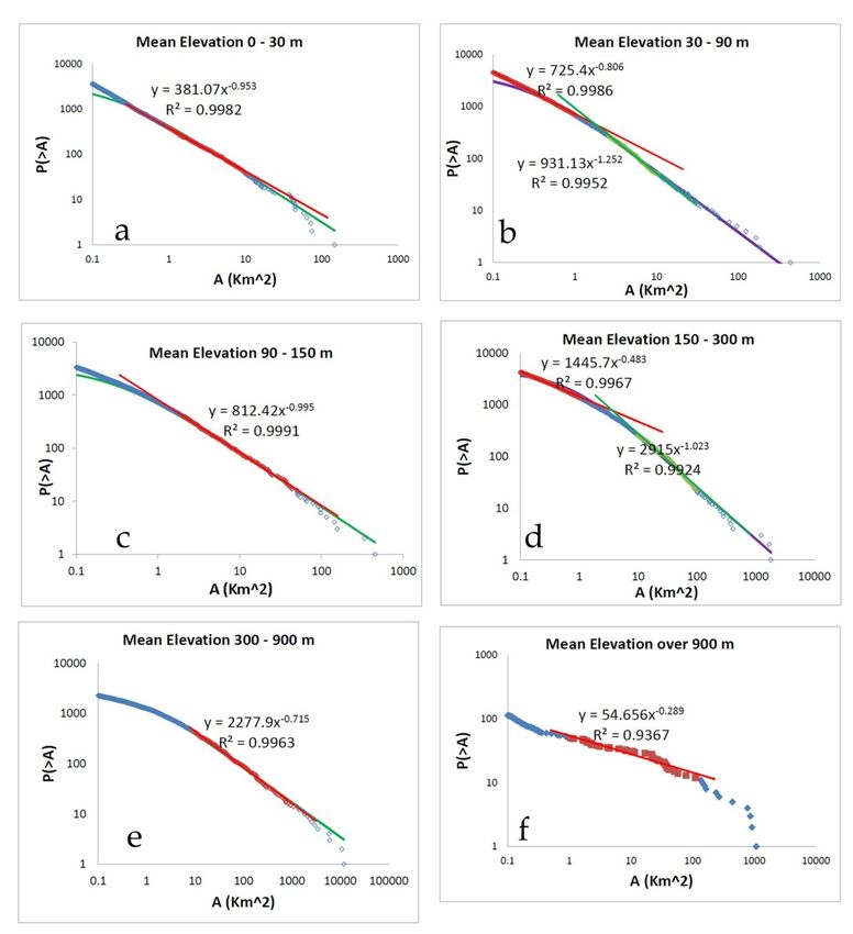
Moreover, having in mind that different elevation values may reflect different landscape dynamics
probably affecting the drainage basins area distribution, zonal statistical analysis was performed on
all the cells of GDEM that belong to each one drainage basin (i.e., zone). In this way, we obtained
the mean elevation value of all the drainage basins in Greece. The latter were classified in 6 classes
according to their mean elevation: 0–30 m, 30–90 m, 90–150 m, 150–300 m, 300–900 m and over 900 m
(Figure 3). The range of each class was adopted from Hammond’s 1964 methodology for classifying
and mapping landforms [53].
Furthermore, the size distribution of Greek drainages classified in several classes according to
their mean value of the Topography Position Index (TPI) [54] is given. The latter is a morphometric
parameter derived from DEM and therefore an objective quantitative way of landform classification
and watersheds characterization. The topographic position index (TPI) was introduced by Weiss (2001)
as a GIS application for landform classification as well as watersheds characterization [55]. The creation
of an ESRI ArcView 3.x extension by Jenness in 2006 [54], led to a broad application of TPI in several
scientific fields, such as geomorphology [56,57]; geology [58]; hydrology [59]; geoarchaeology [60] risk
management [61]. The TPI is defined as:
X
TPIi = M0 − n−1 Mn /n
where M0 is the elevation of the model point under evaluation, Mn the elevation of grid, and n the
total number of surrounding points employed in the evaluation.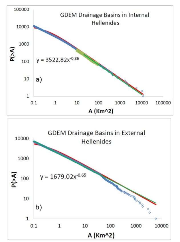
inversion of Mesozoic basins in the northern margin of Apulia as well as the formation of a series of thrust
sheets comprising the External Hellenides thrust belt ([48] and references therein). To search the possible
connection of drainages hierarchy with the geotectonic environment as indicated in a number of
previous works [21,23,24,46,47] we select to search the drainage distribution in the two drainage
subsets
Appl.      defined
      Sci. 2020,      by the two main tectonic patterns of Greece.
                 10, 248                                                                               7 of 18

Appl. Sci. 2019, 9, x FOR PEER REVIEW                                                                         7 of 17

(Figure 3). The range of each class was adopted from Hammond’s 1964 methodology for classifying
and mapping landforms [53].
           Figure 2. Map of Greece showing the division of Hellenides in External and Internal ones.
           Figure 2. Map of Greece showing the division of Hellenides in External and Internal ones.

     Moreover, having in mind that different elevation values may reflect different landscape dynamics
probably affecting the drainage basins area distribution, zonal statistical analysis was performed on all
the cells of GDEM that belong to each one drainage basin (i.e., zone). In this way, we obtained the
mean elevation value of all the drainage basins in Greece. The latter were classified in 6 classes
according to their mean elevation: 0–30 m, 30–90 m, 90–150 m, 150–300 m, 300–900 m and over 900 m

                 Figure 3. Drainage basins classification according to their mean elevation value.
                  Figure 3. Drainage basins classification according to their mean elevation value.
      TPI compares the elevation of each cell in a DEM to the mean elevation of a specified neighborhood
     Furthermore,
around               the size
         that cell. Mean      distribution
                          elevation         of Greek
                                     is subtracted   drainages
                                                   from           classified
                                                          the elevation      in several
                                                                         value          classes
                                                                                at center.       according to their
                                                                                            The neighborhood     size
mean   value    of the  Topography     Position  Index   (TPI)  [54]  is given.  The   latter is
is substantial for the analysis and is related to the scale of landscape feature being analyzed.  a morphometric
                                                                                                         To identify
parameter    derived
large landforms,       fromcircular
                    a large DEM and      therefore anisobjective
                                     neighborhood       proposedquantitative     waythe
                                                                    [56]. Choosing     of correct
                                                                                           landform   classification
                                                                                                   neighborhood     is
and watersheds characterization. The topographic position index (TPI) was introduced by Weiss (2001)
as a GIS application for landform classification as well as watersheds characterization [55]. The creation
of an ESRI ArcView 3.x extension by Jenness in 2006 [54], led to a broad application of TPI in several
scientific fields, such as geomorphology [56,57]; geology [58]; hydrology [59]; geoarchaeology [60] risk
management [61]. The TPI is defined as: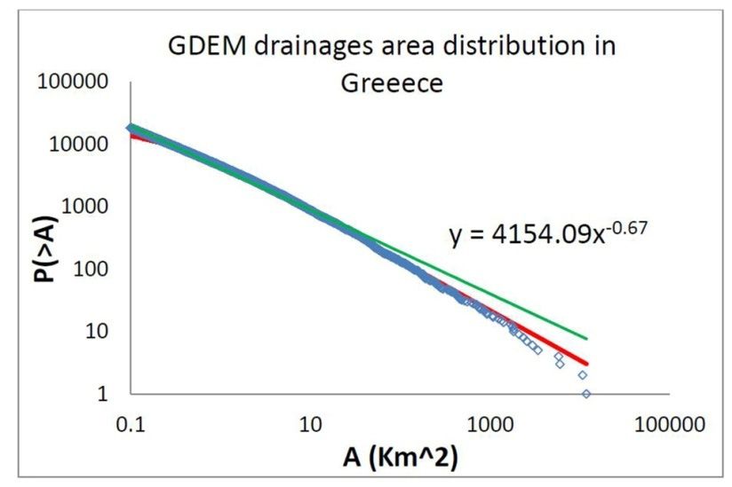
Appl. Sci. 2020, 10, 248                                                                                      8 of 18

an iterative process with several trials before the most appropriate size of neighborhood is decided.
In this study, TPI generated from 2000 m neighborhoods due to the extended spatial coverage of the
study area. Positive TPI values represent areas that are higher than the average of their neighborhoods
(ridges), while negative TPI values represent locations with less elevation than their neighborhood
(valleys). TPI values near zero are characterized as flat areas or areas of constant slope. The mean
TPI value was further calculated for each drainage basin unit. At the scale of 2000 m, TPI reflects
the broader valley morphology and the relative relief of streams and their surrounding topography.
Drainage basins with higher mean values have a high proportion of streams in relatively deeper
and narrower drainages, with narrowness defined by the spatial scale of the index [55]. For the area
distribution analysis we obtained 5 classes of drainage basins with different mean TPI values using the
Appl. Sci. 2019, 9, x FOR PEER REVIEW                                                             8 of 17
quantile classification method (Figure 4a,b).

      Figure 4. (a) TPI values in Greece at a scale of 2000m. Inset: Detail of the TPI map with drainage basins
      Figure 4. (a) TPI values in Greece at a scale of 2000m. Inset: Detail of the TPI map with drainage basins
      overlay, (b) Quantile classification of drainage basins according to their mean TPI value. Inset: detail
      overlay, (b) Quantile classification of drainage basins according to their mean TPI value. Inset: detail
      of the map.
      of the map.
       As a first step in our analysis we present the cumulative drainage area distribution for all the
 territoryaof
      As    first step (Figure
              Greece    in our analysis we present
                               5). As Figure        the cumulative
                                             5 presents a power lawdrainage
                                                                    scaling ofarea
                                                                               the distribution
                                                                                   form [2]     for all the
territory of Greece (Figure 5). As Figure 5 presents a power law scaling of the form [2]
                                                            −β
                                                  N(>A)
                                                   N(>A)~ ~AA -β,,                                                (6)(6)
where
where N(>A)
         N(>A)isis the
                    the number
                        number of
                                of drainages with area greater than A, is
                                                                       is observed
                                                                          observed with
                                                                                    with ββall
                                                                                           all≈0.67,
                                                                                               ≈0.67,with
                                                                                                     with aa
deviation
deviation from
            from power
                  power law
                          law to
                              to observed
                                 observed for
                                          for large drainage areas.
       A power law (see Equation (6)) fits the data for both the data sets organized for the drainage
areas in external and internal Hellenides, respectively, implying a hierarchical organization of drainage
basins. For each one of the cases we have βext ≈ 0.65 and βint ≈ 0.86 (see Figure 6a,b). For the case of
External Hellenides a deviation of observation from power law is observed for large drainage areas,
i.e., for A > 100 km2 .
territory of Greece (Figure 5). As Figure 5 presents a power law scaling of the form [2]
N(>A) ~ A-β, (6)
where N(>A) is the number of drainages with area greater than A, is observed with βall≈0.67, with a
Appl. Sci. 2020,
deviation from10, 248
power law to observed for large drainage areas. 9 of 18
Appl. Sci. 2019, 9, x FOR PEER REVIEW 9 of 17
basins. For each one of the cases we have βext ≈ 0.65 and βint ≈ 0.86 (see Figure 6a,b). For the case of
External Hellenides a deviation of observation from power law is observed for large drainage areas,
i.e., for A > 5.
Figure 100 km
The
2.
drainage area distribution for Greece. A power law fitting is presented with β ≈0.67 all
Figure 5. The
(green line) drainage
along areaQ-exponential
with the distribution for
(redGreece. A power
line) with law
Q≈ 2.41 fitting
(see text).is presented with βall≈0.67
(green line) along with the Q-exponential (red line) with Q≈ 2.41 (see text).
A power law (see Equation (6)) fits the data for both the data sets organized for the drainage areas
in external and internal Hellenides, respectively, implying a hierarchical organization of drainage
Figure 6. The drainage distribution for Internal (a) and External (b) Hellenides, Greece. A power law
Figureis6.presented
fitting The drainage
with distribution for βInternal
βint ≈ 0.86, and (a) and External (b) Hellenides, Greece. A power law
ext ≈ 0.65 for the internal and external Hellenides, respectively
(green line) along with the Q-exponential (red line)for
fitting is presented with βint ≈ 0.86, and β ext ≈ 0.65 theQinternal
with and external Hellenides, respectively
int ≈ 2.16 and Qext ≈ 2.45 for the internal and
(green line)
external along with
Hellenides, the Q-exponential
respectively (see text).(red line) with Qint ≈ 2.16 and Qext ≈ 2.45 for the internal and
external Hellenides, respectively (see text).
In Table 1 we present the power law exponent β observed for each of the six elevation classes
In Table
defined 1 we
(Figure 7). present the power law exponent β observed for each of the six elevation classes
defined (Figure 7).Appl. Sci. 2020, 10, 248 10 of 18
Table 1. The power law exponent β, the Q and q non extensive parameters and the βcal value as
estimated for each of elevation class of Greece drainages.
Mean Elevation β Q q βcal
0–30 m 0.95 1.91 1.48 1.10
30–90 m 1.25 1.85 1.46 1.18
90–150 m 0.995 1.98 1.495 1.02
150–300 m 1.02 2.00 1.5 1.00
300–900
Appl. Sci. 2019, 9, x FOR PEER m
REVIEW 0.715 2.45 1.59 0.69 10 of 17
>900 m 0.29 - - -
Figure 7. The drainage distribution for the six elevation classes defined in Greece. A power law fitting
Figure 7. Thealong
is presented drainage
withdistribution for the sixThe
the Q-exponentials. elevation
scalingclasses defined
exponent in the
β and Greece. A power
Q values law fitting
as presented in
is presented along
Table 1 (see text). with the Q-exponentials. The scaling exponent β and the Q values as presented in
Table 1 (see text).
In Table 2 we present the power law exponent β observed for each of TPI defined classes
Table 1.8).The power law exponent β, the Q and q non extensive parameters and the βcal value as
(see Figure
estimated for each of elevation class of Greece drainages.
Mean Elevation β Q q βcal
0–30 m 0.95 1.91 1.48 1.10
30–90 m 1.25 1.85 1.46 1.18
90–150 m 0.995 1.98 1.495 1.02
150–300 m 1.02 2.00 1.5 1.00
300–900 m 0.715 2.45 1.59 0.69Appl. Sci. 2020, 10, 248 11 of 18
Table 2. The power law exponent β, the Q and q non extensive parameters and the βcal value as
estimated for each TPI class.
TPI Class β Q q βcal
Class 1 (valleys) 1.87 1.38 1.275 2.6
Class 2 1.28 1.68 1.405 1.47
Class 3 (nearly flat areas or areas of constant slope) 0.69 2.40 1.58 0.71
Class 4 0.78 2.27 1.56 0.79
Class 5 (ridges)
Appl. Sci. 2019, 9, x FOR PEER REVIEW 1.27 1.60 1.375 1.67 11 of 17
Figure 8. The drainage distribution for the five classes defined in Greece according to TPI values.
Figure
A power8.The
lawdrainage
fitting isdistribution for the
presented along fivethe
with classes defined in Greece
Q-exponentials. according
The scaling to TPI
exponent β values.
and theAQ
power law fitting is presented along with
values as presented in Table 2 (see text). the Q-exponentials. The scaling exponent β and the Q values
as presented in Table 2 (see text).
All the above mentioned distributions are analyzed in terms of Tsallis entropy estimating the
Table 2.
q-entropic The characterizing
index power law exponent β, the Q andToq estimate
the distribution. non extensive parameters
the q value and the βcal the
(or equivalently value as we
Q one)
estimated for each TPI class.
fit all the observed drainage areas distributions with Equation (4). In Figures 5 and 6 the Q-exponential
TPI Class β Q q βcal
Class 1 (valleys) 1.87 1.38 1.275 2.6
Class 2 1.28 1.68 1.405 1.47
Class 3 (nearly flat areas or areas of constant slope) 0.69 2.40 1.58 0.71
Class 4 0.78 2.27 1.56 0.79Appl. Sci. 2020, 10, 248 12 of 18
fitting leads to the Q (and equivalently q) values that describe the drainage distribution as Qall ≈ 2.41,
Qint ≈ 2.16, Qext ≈ 2.45 or equivalently qall = 1.58, qint = 1.54 and qext = 1.59, for all the drainages of
Greece, and for that in the internal and external Hellenides, respectively. Since the theoretical β value
is given as
1
βcal =
Q−1
the calculated β values using the Q estimates are βcal all
≈0.71, βcal
int
≈0.86 and βcal
ext ≈0.69 for the drainages
all over Greece, and for that in the internal and external Hellenides, respectively, in agreement with
that estimated fitting an empirical power law in the distribution. The same procedure is repeated for
all the data subsets created by the classification of the Greece drainages. In Tables 1 and 2 the Q and q
parameters along with the βcal values are given.
5. Discussion
In the present work we study the hierarchical pattern of drainages area distribution in Greece as
extracted from an ASTER GDEM v2 Digital Elevation Model, offering a 30m resolution, enabling the
creation of an accurate drainage basins’ database within a GIS environment. The power law exponent β
for classification of drainages based on a) the geotectonic pattern and b) on topographic characteristics
are estimated. Our analysis, demonstrate that an empirical power law distribution could be used
to describe, as a first approximation, the drainages’ area distribution. We study the drainage basin
area-frequency distribution in the set of Greek drainages along with the subsets constructed applied
different geological or geomorphological criteria. The hierarchy pattern observed for the drainage’s
areas not only for all the Greece but also for the subsets of drainages in the internal and external
Hellenides that are the main tectonic structures in Greece, and the drainages classified according to
their elevation or the Topographic Position Index (TPI), was presented.
Furthermore the feasibility of the non-extensive statistical physics applied to the size distribution
of the drainages areas is demonstrated. The estimation of the entropic parameter q which is mainly in
the range 1.45–1.55, indicates a sub-additive system, with significant long range interactions. Within
the view of Tsallis entropy we extract as a first approximation of Q-exponential a power law of the form
1
N(> A) ∼ A−β where β =
Q−1
with Q the non-extensive parameter extracted from the fitting of observations with a Q-exponential.
The Q parameter is related with the q entropic Tsallis parameter introduced in the definition of Tsallis
Entropy as
1
q = 2− .
Q
Following NESP, the Greek drainage system could be seen as a drainage set organized by the
merging of different sub-systems, according to the classification used. In view of Tsallis statistics
formulation for non-extensive systems composed of non-extensive subsystems having different Q’s it
is proposed in [62] and references therein, that enables to estimate the behavior of a composite system
containing subsystems, each having its own Q, using the expression [62]:
P
Q lnNi
Q= P i
lnNi
where Qi the Q-exponential parameter and Ni the number of elements (drainages) in each of the
sub-sets formed the composite one. In this frame the Greek drainage system could be viewed asAppl. Sci. 2020, 10, 248 13 of 18
containing two Q-exponential subsystems with different Q’s as the external and internal Hellenides
drainage sets are. Since Qint < Q < Qext an estimation of Q is given
Qint lnNint + Qext lnNext
Q= , where Nint = 11042 and Next = 7076,
lnNint + lnNext
the number of drainages in each subset. Substituting the values of Qint and Qext we lead to Q = 2.30 in a
good agreement with Q ≈ 2.41 obtained with fitting a Q-exponential for all the Greek drainage system.
We now discuss the possible origin of the deviation from the power law observed in a number of
cases for large values of drainage area A, where an exponential tail (i.e., q = 1) observed. According to
NESP the generalized probability distribution
!
A
p = p(A) ∝ expq (− )
Aq
can be obtained by solving the nonlinear differential equation
dp 1
= −βq pq , where βq = and q , 1;
dA Aq
while Boltzmann-Gibbs (BG) are approached, with the BG entropy optimized when q = 1.
We now use the above differential equation path in order to further generalize the anomalous
equilibrium distribution, in such a way as to have a crossover from anomalous (q , 1) to normal
(q = 1) statistical mechanics, while increasing the drainage’s area. Following [63] we consider the
differential equation
dp
= −β1 p − βq − β1 pq ,
dA
whose solution is
1
− q−1
βq βq
(q−1)β1 A
p(A) = C [ 1 − + e ] , (7)
β1 β1
where C is a normalization factor. For positive βq and β1 , p(A) decreases monotonically with increasing
A. It can be easily verified that in the case where βq >> β1 , equation (7) defines three regions, according
to the area A of the drainage. We will call these “drainage regions”, small, intermediate and large
drainage area regions, respectively. The asymptotic behavior of the probability distributions in these
areas is
1 1
p(A) ∝ 1 − βq Afor 0 ≤ A ≤ Ac1 where Ac1 = ,
q − 1 βq
h i −1 − 1 1 1
p(A ) ∝ (q − 1)βq (q−1) A (q−1) for Ac1 ≤ A ≤ Ac2 where Ac2 = ,
q − 1 β1
1
β (q−1) −β1 A
p(A) ∝ ( 1 ) e for A ≥ Ac2 ,
βq
where Ac1 and Ac2 are the cross-over points between the three regions.
The observed crossover from hierarchical (q , 1) to exponential (q = 1) pattern, with increasing of
the parameter A deserves special attention. In this case, in equation (7) expanding the exponential
term in it can be easily concluded that in the case where (q − 1)β1 A
1 the asymptotic behavior of
the probability distributions simplified as a q-exponential
1
p(A) C expq (−βq A) for A < Ac = , (8a)
[(q − 1)β1 ]Appl. Sci. 2020, 10, 248 14 of 18
while
" # −1
β (q−1)
p(A) ∝ 1 e−β1 A for A ≥ Ac , (8b)
βq
where Ac is the crossover point between the hierarchical (q , 1) to exponential (q = 1) statistical
mechanics. Equation (8a) leads to the q-exponential of Equation (6) for a cumulative distribution
function P(> A). The latter Equation (8a,b) explain the q-exponential description of the distribution of
drainage areas along with the exponential tail observed in some of the cases, as a result of generalized
non-extensive statistical mechanics.
Here we state that the estimation of the entropic parameter q which is mainly in the range
1.45–1.55, indicates a sub-additive system, with significant long range interactions. The q non-extensive
parameter increases as the mean elevation increases, implying that watersheds in higher elevations
interact stronger than those of lower mean elevations. These strong interactions are probably related to
the limited space in which they have to be developed. As a result, the area distribution between smaller
and bigger basins follows a hierarchical pattern. On the other hand, watersheds of low elevation
are more sensitive to tectonic (presence of faults), climatic (precipitation) and antropogenic (land use
changes) factors.
As for the q parameter extracted from the TPI subdata sets, there is an obvious increase from class
1 (big negative values, showing watersheds that are relatively deeper and narrower with a broader
valley morphology) to class 2 and class 3. According to [55] watersheds of class 1 can be more sensitive
to drainage wide deforestation and land use, and would likely have a stronger response to extreme
weather and snowmelt events. This fact is in a good agreement with a q equal to 1.275. As the TPI
values increase to class 4 and class 5, the q parameter value decreases, implying weaker interactions
between basins of a broader ridge topography. The biggest q value has been estimated for class 3
(nearly flat areas or areas of constant slope) indicating that in such environments of small roughness the
systems are well organized with their area distribution to follow a hierarchy (mature or old drainage
basins?).
6. Concluding Remarks
Summarizing we can state that the use of non-extensive statistical physics is a suited tool to describe
the drainages frequency-size (area) distribution. The obtained distribution function incorporates the
characteristics of non-extensivity into the cumulative distribution of drainages’ areas and explains the
observed power law behavior fitting the observed data. The presence of deviations from the power
law for large areas in the frequency distribution can be regarded as the manifestation of the physical
foundation of the generalized non-extensive Tsallis entropy, where the deviation of distribution from
power law for large drainages area is discussed in terms of generalized non extensive statistical
mechanics, introducing two mechanisms that describe hierarchical and exponential patterns. The latter
implies two main mechanisms applied to form the geomorphological drainage pattern. The first one
for the intermediate size drainages where a power law applies and a second one for the large drainage
areas, where a significant lower frequency observed compared with that calculated by the power law
extrapolation. In addition our work contributes, supporting the ideas of scaling and universality in
geomorphology as presented in [64,65] using an entropic approach as presented in [28].
Note that the proposed scaling is not an empirical guess for the drainages size distribution but
derived from the first principle of non-extensive entropy formalism, which is completely universal
and has a long range of application [28,34,36]. The physical meaning underlying the non-extensive
entropy formalism is that the final physical state can be considered as a collection of interacted parts
which, after division, have the sum of individual entropies larger than the entropy of the initial state inAppl. Sci. 2020, 10, 248 15 of 18
a similar way as pointed out for landslides and rockfalls [29,30,38]. The latter is straightforward from
the concept of not additivity since [28,29,36,38,62].
X
S(Vi ) > S(∪Vi )
i
Finally, since drainage systems consists of many non-independent subareas, the non-additivity
index q (q > 1) could be interpreting as an approximate measure of the long-range interactions within
the drainage system. The scaling properties studied in this work and in the theory developed in
order to explain the experimental evidence of power law distribution it is expected to be applied
in hydrological applications and it could be proved significantly helpful for geomorphologists and
engineers in order to validate water flows within a drainage basin.
Author Contributions: Conceptualization, F.V.; Formal analysis, F.V. and M.K.; Investigation, M.K.; Methodology,
F.V.; Resources, M.K.; Software, M.K.; Validation, F.V.; Visualization, M.K.; Writing—original draft, F.V. and
M.K.; Writing—review & editing, F.V. and M.K. All authors have read and agreed to the published version of
the manuscript.
Funding: We acknowledge support of this work by the project “HELPOS – Hellenic System for Lithosphere
Monitoring, Greece” (MIS 5002697) which is implemented under the Action “Reinforcement of the Research and
Innovation Infrastructure”, funded by the Operational Programme “Competitiveness, Entrepreneurship and
Innovation, Greece” (NSRF2014–2020) and co-financed by Greece and the European Union (European Regional
Development Fund).
Conflicts of Interest: The authors declare no conflict of interest.
References
1. Bak, P. Complexity and criticality. In How Nature Works; Copernicus: New York, NY, USA, 1996; pp. 1–32.
2. Newman, M.E.J. Power laws, Pareto distributions, and Zipf’s law. Contemp. Phys. 2005, 46, 323–351.
[CrossRef]
3. Preobrazhenskiy, V.S. Geosystem as an object of landscape study. GeoJournal 1983, 7, 131–134. [CrossRef]
4. McDonnell, J.J.; Sivapalan, M.; Vaché, K.; Dunn, S.; Grant, G.; Haggerty, R.; Hinz, C.; Hooper, R.; Kirchner, J.;
Roderick, M.L.; et al. Moving beyond heterogeneity and process complexity: A new vision for watershed
hydrology. Water Resour. Res. 2007, 43. [CrossRef]
5. Malamud, B.D.; Morein, G.; Turcotte, D.L. Forest fires: An example of self-organized critical behavior. Science
1998, 281, 1840–1842. [CrossRef] [PubMed]
6. Codilean, A.T.; Bishop, P.; Hoey, T.B. Surface process models and the links between tectonics and topography.
Prog. Phys. Geogr. 2006, 30, 307–333. [CrossRef]
7. Malavieille, J. Impact of erosion, sedimentation, and structural heritage on the structure and kinematics of
orogenic wedges: Analog models and case studies. GSA Today 2010, 20, 4–10. [CrossRef]
8. Graveleau, F.; Dominguez, S. Analogue modelling of the interaction between tectonics, erosion and
sedimentation in foreland thrust belts. C. R. Geosci. 2008, 340, 324–333. [CrossRef]
9. Roe, G.H. Orographic precipitation. Annu. Rev. Earth Planet. Sci. 2005, 33, 645–671. [CrossRef]
10. Van der Beek, P.A.; Champel, B.; Mugnier, J.L. Control of detachment dip on drainage development in
regions of active fault propagation folding. Geology 2002, 30, 471–474. [CrossRef]
11. Hovius, N. Regular spacing of drainage outlets from linear mountain belts. Basin Res. 1996, 8, 29–44.
[CrossRef]
12. Jordan, T.E. Thrust loads and foreland basin evolution, Cretaceous, western United States. Am. Assoc. Pet.
Geol. Bull. 1981, 65, 2506–2520.
13. Persson, K.S.; Garcia-Castellanos, D.; Sokoutis, D. River transport effects on compressional belts: First results
from an integrated analogue-numerical model. J. Geophys. Res. 2004, 109. [CrossRef]
14. Bishop, P. Drainage rearrangement by river capture, beheading and diversion. Prog. Phys. Geogr. 1995,
19, 449–473. [CrossRef]Appl. Sci. 2020, 10, 248 16 of 18
15. Dorsey, R.J.; Roering, J.J. Quaternary landscape evolution in the San Jacinto fault zone, Peninsular Ranges
of Southern California: Transient response to strike-slip fault initiation. Geomorphology 2006, 73, 16–32.
[CrossRef]
16. Garcia-Castellanos, D.; Estrada, F.; Jiménez-Munt, I.; Gorini, C.; Fermàndez, M.; Vergés, J.; De Vicente, R.
Catastrophic flood of the Mediterranean after the Messinian salinity crisis. Nature 2009, 462, 778–781.
[CrossRef]
17. Vörösmarty, C.V.; Federer, C.A.; Schloss, A.L. Potential evaporation functions compared on US watersheds:
Possible implications for global-scale water balance and terrestrial ecosystem modeling. J. Hydrol. 1998,
207, 147–169. [CrossRef]
18. Dhakal, A.S.; Sidle, R.C. Distributed simulations of landslides for different rainfall conditions. Hydrol. Process.
2004, 18, 757–762. [CrossRef]
19. Lazzari, M.; Geraldi, E.; Lapenna, V.; Loperte, A. Natural hazards vs. human impact: An integrated
methodological approach in geomorphological risk assessment on the Tursi historical site, Southern Italy.
Landslides 2006, 3, 275–287. [CrossRef]
20. Lee, K.T.; Lin. Y.T. Flow analysis of landslide dammed lake water sheds a case study. J. Am. Water
Resour. Assoc. 2006, 42, 1615–1628. [CrossRef]
21. Yang, D.Q.; Zhao, Y.Y.; Armstrong, R. Streamflow response to seasonal snow cover mass changes over large
Siberian watersheds. J. Geophys. Res. Earth Surf. 2007, 112, F2. [CrossRef]
22. Strahler, A.H. Modern Physical Geography; John Wiley & Sons: New York, NY, USA, 1983; p. 532,
ISBN 9780471081050.
23. Rodriguez-Iturbe, I.; Ijjasz-Vasquez, E.J.; Bras, R.L.; Tarboton, D.G. Power law distributions of mass end
energy in river basins. Water Resour. Res. 1992, 28, 988–993. [CrossRef]
24. Inaoka, H.; Takayasu, H. Water erosion as a fractal growth process. Phys. Rev. E 1993, 47, 126–132. [CrossRef]
[PubMed]
25. Veitzer, S.; Troutman, B.; Gupta, V. Power-law tail probabilities of drainage areas in river basins. Phys. Rev. E
2003, 68, 016123. [CrossRef] [PubMed]
26. Fehr, E.; Kadau, D.; Araujo, N.A.M.; Andrade, J.S.; Herrmann, H.J. Scaling relations for watersheds.
Phys. Rev. Lett. 2011, 84, 036116. [CrossRef] [PubMed]
27. Tsallis, C. Nonextensive statistics: Theoretical, Experimental and Computational Evidences and Connections.
Braz. J. Phys. 1999, 29, 1–35. [CrossRef]
28. Tsallis, C. Introduction to Nonextensive Statistical Mechanics: Approaching a Complex World; Springer:
Berlin/Heidelberg, Germany, 2009.
29. Vallianatos, F. A non-extensive approach to risk assessment. Nat. Hazards Earth Syst. Sci. 2009, 9, 211–216.
[CrossRef]
30. Vallianatos, F. On the statistical physics of rockfalls: A non-extensive view. EPL 2013, 101, 10007. [CrossRef]
31. Vallianatos, F.; Sammonds, P. Is plate tectonics a case of non-extensive thermodynamics? Phys. A Stat.
Mech. Appl. 2010, 389, 4989–4993. [CrossRef]
32. Vallianatos, F.; Sammonds, P. A non-extensive statistics of the fault-population at the Valles Marineris
extensional province, Mars. Tectonophysics 2011, 509, 50–54. [CrossRef]
33. Vallianatos, F.; Michas, G.; Papadakis, G.; Sammonds, P. A non extensive statistical physics view to the
spatiotemporal properties of the June 1995, Aigion earthquake (M6.2) aftershock sequence (West Corinth rift,
Greece). Acta Geophys. 2012, 60, 758–768. [CrossRef]
34. Vallianatos, F.; Papadakis, G.; Michas, G. Generalized statistical mechanics approaches to earthquakes and
tectonics. Proc. R. Soc. A Math. Phys. Eng. Sci. 2016, 472, 20160497. [CrossRef] [PubMed]
35. Vallianatos, F.; Michas, G.; Papadakis, G. Nonextensive statistical seismology: An overview. In Complexity of
Seismic Time Series; Elsevier: Berlin/Heidelberg, Germany, 2018; pp. 25–59.
36. Vallianatos, F.; Telesca, L. (Eds.) Statistical Mechanics in Earth Physics and Natural Hazards. Acta Geophys.
2012, 60, 499. [CrossRef]
37. Telesca, L. Nonextensive analysis of seismic sequences. Phys. A Stat. Mech. Appl. 2010, 389, 1911–1914.
[CrossRef]
38. Chen, C.; Telesca, L.; Lee, C.T.; Sun, Y.S. Statistical physics of landslides: New paradigm. EPL 2011, 95, 49001.
[CrossRef]Appl. Sci. 2020, 10, 248 17 of 18
39. Iwahashi, J.; Pike, R.J. Automated classifications of topography from DEMs by an unsupervised nested-means
algorithm and a three-part geometric signature. Geomorphology 2007, 86, 409–440. [CrossRef]
40. De Reu, J.; Bourgeois, J.; Bats, M.; Zwertvaegher, A.; Gelorini, V.; De Smedt, P.; Chu, W.; Antrop, M.;
De Maeyer, P.; Finke, P.; et al. Application of the topographic position index to heterogeneous landscapes.
Geomorphology 2013, 186, 39–49. [CrossRef]
41. Tachikawa, T.; Kaku, M.; Iwasaki, A.; Gesch, D.B.; Oimoen, M.J.; Zhang, Z.; Danielson, J.J.; Krieger, T.;
Curtis, B.; Haase, J.; et al. ASTER Global Digital Elevation Model Version 2—Summary of Validation Results.
2011, NASA. Available online: http://pubs.er.usgs.gov/publication/70005960 (accessed on 1 December 2018).
42. Rexer, M.; Hirt, C. Comparison of free high-resolution digital elevation data sets (ASTER GDEM2, SRTM
v2.1/v4.1) and validation against accurate heights from the Australian National Gravity Database. Aust. J.f
Earth Sci. 2014, 61, 213–226. [CrossRef]
43. Das, S.; Patel, P.P.; Sengupta, S. Evaluation of different digital elevation models for analyzing drainage
morphometric parameters in a mountainous terrain: A case study of the Supin–Upper Tons Basin, Indian
Himalayas. SpringerPlus 2016, 5, 1544. [CrossRef]
44. Wu, S.; Li, J.; Huang, G.H. A study on DEM-derived primary topographic attributes for hydrologic
applications: Sensitivity to elevation data resolution. Appl. Geogr. 2008, 28, 210–223. [CrossRef]
45. O’Callaghan, J.; Mark, D. The extraction of drainage networks from digital elevation data. Comput. Vis.
Graph. Image Proc. 1984, 28, 323–344. [CrossRef]
46. Wang, X.M.; Wang, P.; Zhang, P.; Hao, R.; Huo, J. Statistical dynamics of early river networks. Phys. A Stat.
Mech. Appl. 2012, 391, 4497–4505. [CrossRef]
47. Zhu, H.; Zhao, Y.; Liu, H. Scale characters analysis for gully structure in the watersheds of loess landforms
based on digital elevation models. Front. Earth Sci. 2018, 12, 431–443. [CrossRef]
48. Papanikolaou, D. Geology of Greece; Eptalofos Publication: Athens, Greece, 1986; p. 240. (In Greek)
49. Papanikolaou, D. Timing of tectonic emplacement of the ophiolites and terrane paleogeography in the
Hellenides. Lithos 2009, 108, 262–280. [CrossRef]
50. Doutsos, T.; Koukouvelas, I.K.; Xypolias, P. A New Orogenic Model for the External Hellenides; Geological
Society Special Publication: London, UK, 2006; Volume 260, pp. 507–520.
51. Kilias, A.; Frisch, W.; Avgerinas, A.; Dunkl, I.; Falalakis, G.; Gawlick, H.J. Alpine architecture and kinematics
of deformation of the northern Pelagonian nappe pile in the Hellenides. Austrian J. Earth Sci. 2010, 103, 4–28.
52. Dilek, Y. Collision tectonics of the Mediterranean region: Causes and consequences. Spec. Pap. Geol. Soc. Am.
2006, 409, 1–13.
53. Hammond, E.H. Analysis of properties in land form geography: an application to broad-scale landform
mapping. Ann. Assoc. Am. Geogr. 1964, 54, 11–19. [CrossRef]
54. Jenness, J. Topographic Position Index (tpi_jen.avx) Extension for ArcView 3.x, v. 1.3a; Jenness Enterprises:
Flagstaff, AZ, USA, 2006.
55. Weiss, A. Topographic position and landforms analysis. In Proceedings of the Poster presentation, ESRI User
Conference, San Diego, CA, USA, 9–13 July 2001.
56. Tagil, S.; Jenness, J. GIS-based automated landform classification and topographic, landcover and geologic
attributes of landforms around the YazorenPolje, Turkey. J. Appl. Sci. 2008, 8, 910–921. [CrossRef]
57. McGarigal, K.; Tagil, S.; Cushman, S. Surfacemetrics: an alternative to patchmetrics for the quantification of
landscape structure. Landsc. Ecol. 2009, 24, 433–450. [CrossRef]
58. Mora-Vallejo, A.; Claessens, L.; Stoorvogel, J.; Heuvelink, G.B.M. Small scale digital soil mapping in
southeastern Kenya. Catena 2008, 76, 44–53. [CrossRef]
59. Francés, A.P.; Lubczynski, M.W. Topsoil thickness prediction at the catchment scale by integration of invasive
sampling, surface geophysics, remote sensing and statistical modeling. J. Hydrol. 2011, 405, 31–47. [CrossRef]
60. Berking, J.; Beckers, B.; Schütt, B. Runoff in two semi-arid watersheds in a geoarcheological context: A case
study of Naga, Sudan, and Resafa, Syria. Geoarchaeology 2010, 25, 815–836. [CrossRef]
61. Platt, R.V.; Schoennagel, T.; Veblen, T.T.; Sherriff, R.L. Modeling wildfire potential in residential parcels:
A case study of the north-central Colorado Front Range. Landsc. Urban Plan. 2011, 102, 117–126. [CrossRef]
62. Vallianatos, F. On the non-extensivity in Mars geological faults. EPL 2013, 102, 28006. [CrossRef]
63. Tsekouras, G.A.; Tsallis, C. Generalized entropy arising from a distribution of q-indices. Phys. Rev. E 2005,
71, 046144. [CrossRef]Appl. Sci. 2020, 10, 248 18 of 18
64. Dodds, P.; Rothman, D.H. Scaling, Universality, and Geomorphology. Annu. Rev. Earth Planet. Sci. 2000,
28, 571–610. [CrossRef]
65. Dodds, P.; Rothman, D.H. Unified View of Scaling Laws for River Networks. Phys. Rev. E. 1999, 59, 4865–4877.
[CrossRef]
© 2019 by the authors. Licensee MDPI, Basel, Switzerland. This article is an open access
article distributed under the terms and conditions of the Creative Commons Attribution
(CC BY) license (http://creativecommons.org/licenses/by/4.0/).You can also read