A Novel Geophysical Soil Loss Model for Erosion Prediction and Monitoring in Anambra, South East, Nigeria
←
→
Page content transcription
If your browser does not render page correctly, please read the page content below
International Journal of Innovative Environmental Studies Research 9(2):11-24, April-June, 2021

          © SEAHI PUBLICATIONS, 2021 www.seahipaj.org                            ISSN: 2354-2918

A Novel Geophysical Soil Loss Model for Erosion Prediction
    and Monitoring in Anambra, South East, Nigeria
                                          1
                                           R.C. Nwankwo & 2E.C. Okoli

                                      1
                                    Department of Physical Sciences,
                         Faculty of Science, Edwin Clark University, Kiagbodo,
                                P.M.B. 101, Ughelli, Delta State, Nigeria
                                 Email: nwankwo_c_rufus@yahoo.com
                               2
                                   Department of Physics, Faculty of Science,
                                    Delta State University, Abraka, Nigeria
                                        Email: okoliepeace@yahoo.com

ABSTRACT
Gully erosion is an environmental problem that has over decades threatened Anambra State as well as
other parts of Nigeria and countries of sub-Saharan Africa. Gullies threaten the soil, water, material
resources and agricultural productivity and cause human losses annually. This study is undertaken to
generate a new geophysical model that is capable of predicting and monitoring vulnerability of
the soil to gully erosion. Conventional Soil Loss Equations/Models, used for calculating annual soil
loss to aid predictions of soil vulnerability to erosion, encapsulate the erodibility factor (a soil parameter)
which constitutes some difficulty in prediction processes. The associated problem is hinged on the fact
that erodibility is relatively difficult to measure and its’ evaluation in any soil erosion prediction modeling
requires some rigorous process that is prone to error. In our new geophysically modified Soil Loss
Equation, the ‘erodibility factor’ has thus been replaced with the ‘rigidity factor’ (a geophysical
parameter) due to its error-free and relative ease of measurement and acquisition. We have used the
power law modeling approach to fit the rigidity modulus with other input variables in order to obtain the
new geophysical soil loss prediction model. Inputting rigidity into our newly modified soil loss equation,
however, requires introduction of a constant λ which eliminates any dimensional problem in the model.
We have called this ‘the area constant’ and it is uniquely characteristic of any given geographic or
geologic area under investigation. The rigidity data used in testing our model were calculated from
existing Vp and Vs values derived from previous works documented in the literature. For the Anambra
Basin which constitutes our study area, we obtained the value of λ as 2.438 x10¹² t2ha-1hr-1MJ-1. Use of
this λ-value in conjunction with the rigidity data and other values in our new equation gave soil loss rates
in the range of 0.013 - 0.067 tha-1yr-1, showing only slight erosion in the study area. We do not claim to
have exhausted this approach. However, we have in this study successfully derived a new geophysical
soil loss model suitable for erosion prediction, monitoring and control in any part of the world.
Keywords: Prediction, monitoring, geophysical, modified, soil, loss, model

1.0 INTRODUCTION
Gully erosion is an environmental problem that has threatened Anambra State over the years as well as
other parts of Nigeria and countries of sub-Saharan Africa. Gullies threaten the soil, water and material
resources and cause human losses annually. It accounts for the severe environmental degradation in
Anambra State and the South-East of Nigeria arising from heavy runoff and soil loss. Solving the erosion
                                                      11
Nwankwo & Okoli ….. Int. J. Innovative Environ. Studies Res. 9(2):11-24, 2021

problem requires accurate prediction, monitoring and conservation practices. Over the decades, various
types of erosion especially gullies have been found to constitute global, continental and national
problems. Soil erosion is a widespread problem throughout Europe, Asia, Africa and rest of the world. A
report for the Council of Europe, using revised GLASOD data (Oldeman et al., 1991; Van Lynden, 1995),
provides an overview of the extent of soil degradation in Europe. Some of the findings indicate that the
most dominant effect is the loss of topsoil, which is often not conspicuous but nevertheless potentially
very damaging. Physical factors like climate, topography and soil characteristics are important in the
process of soil erosion. In part, this explains the difference between the severe water erosion problem in
Iceland and the much less severe erosion in Scandinavia where the climate is less harsh and the soils are
less erodible. The Mediterranean region is particularly prone to erosion. This is because it is subject to
long dry periods followed by heavy bursts of erosive rainfall, falling on steep slopes with fragile soils,
resulting in considerable amounts of erosion. This contrasts with NW Europe where soil erosion is slight
because rain falling on mainly gentle slopes is evenly distributed throughout the year (Morgan, 1992).

Many methods of soil erosion prediction modelling have been developed. These include deterministic,
stochastic, multivariate statistical modeling, integrated modeling approach as well as the use of the
conventional Universal Soil Loss Equation (USLE). These models can be used in varied ways; either for
mapping and predicting areas prone to erosion or calculating soil loss rates that facilitate prediction and
monitoring. Mapping of soil loss in a degraded area has been achieved through the use of the Geographic
Information System (GIS). The models have various distinctions and subdivisions in terms of application
depending on global, continental/regional or national scale needs. Erosion models have therefore evolved
in a number of ways based on the scale for which a model can be used. Some models have been designed
to predict long-term annual soil losses, while others predict single storm losses (event-based).
Alternatively, lumped models have been developed which predict erosion at a single point and spatially
distributed models which predict erosion over a large area. The choice for a particular model largely
depends on the purpose for which it is intended and the availability of data, time and money.
Jäger (1994) used the empirical Universal Soil Loss Equation (USLE) to assess soil erosion risk in
Baden-Württemberg (Germany). De Jong (1994) used the Morgan, Morgan and Finney model (Morgan et
al., 1984) as a basis for his SEMMED model. Input variables were derived from standard meteorological
data, soil maps, multitemporal satellite imagery, digital elevation models and a limited amount of field
data. In this way, the SEMMED model has been used to produce regional erosion risk maps of parts of
the Ardêche region and the Peyne catchment in Southern France (De Jong, 1994, De Jong et al., 1998).

Kirkby and King (1998) assessed soil erosion risk for the whole of France using a model-based approach.
Their model provides a simplified representation of erosion in an individual storm. The model contains
terms for soil erodibility, topography and climate. All storm rainfall above a critical threshold (whose
value depends on soil properties and land cover) is assumed to contribute to runoff, and erosion is
assumed to be proportional to runoff. Monthly and annual erosion estimates are obtained by integrating
over the frequency distribution of rainstorms.
The Universal Soil Loss Equation (USLE) (Wischmeier & Smith, 1978) has also been developed and
applied both on the global, regional and national scale for assessing erosion risks. Even though a wide
variety of models are available for erosion risk assessment purposes, most of them simply require so
much input data that applying them at the various scales becomes problematic. The well-known Universal
Soil Loss Equation is used because it is one of the least data demanding erosion models that has been
applied widely at different scales. The USLE is a simple empirical model, based on regression analyses of
soil loss rates on erosion plots. The model is designed to estimate long-term annual erosion rates on
agricultural fields. Although the equation has some shortcomings and limitations, it represents a
standardised approach and has been widely applied at the global, continental and national scales because
of its relative simplicity and robustness.

                                                    12
Nwankwo & Okoli ….. Int. J. Innovative Environ. Studies Res. 9(2):11-24, 2021
In Sub-Sahara Africa and particularly Anambra, South-east region of Nigeria, erosion especially the
gullying type has produced periodic devastating human losses, cut off roads that inhibited vehicular
movements, reduced agricultural productivity and led to loss of lands that otherwise would have been
available for various uses. Ofomata (1981, 1985) has explained that gully erosion types are the most
visible forms of erosion in Nigeria mainly because of the remarkable impression they leave on the surface
of the earth. He remarked that more than 1.6% of the entire land area of eastern Nigeria is occupied by
gullies. The classical gully sites in the region are located at Agulu, Nanka, Ozuitem, Oko, Isuikwuato and
Orlu. With the increased developmental activities, the number and magnitudes of gullies have escalated in
the region, with more than 600 active sites.
Most researchers have found that the environmental factors of vegetation, geology, geomorphology,
climate (rainfall) which is very aggressive in the region and the soil factor have necessitated the use of the
conventional USLE model for assessing and predicting erosion risk in the region. Like many other
models, the USLE model takes into account these environmental parameters as well as the
conservation/support practice factor. In South-east Nigeria particularly Anambra State, soil geology has
been found to be one of the dominant factors that induce gullies in the area. This accounts for the capture
of soil geology in the form of the erodibility term in the USLE model. However, erodibility, amongst the
other erosion-inducing factors, has been proved to be difficult to measure. Hence evaluation of soil loss
rate can be error-prone when erodibilty is used as an input in a model. To solve this problem, the soil
rigidity factor can be used as an input other than the soil erodibility factor. Soil rigidity is an elastic
geophysical parameter that, like the erodibility factor, represents a measure of soil strength and therefore
determines the ease with which soil can be eroded.
Rigidity and other elastic rock properties are sources of valuable information for most projects in rock
mechanics as the knowledge of deformational characteristics of rocks is paramount in the design and
construction of any structure on the rock or soil (Atat et al, 2012).The rigidity data can therefore be used
as an input in soil loss prediction modeling rather than the erodibility factor. The soil rigidity, also known
as rigidity or shear modulus, can be obtained from combined s- and p-wave velocities using appropriate
relations. Field acquisition of s- and p-wave velocities from the top soil in a geologic area can be achieved
using the seismic refraction method which utilizes the propagation of waves through the earth that are
eventually collected by appropriate detectors placed systematically on the earth’s surface (Grant and
West, 1965; Bullen and Bruce, 1993). With the velocities of the s-waves and p-waves known, the rigidity
of the medium of propagation can be found. Acquisition of rigidity data thus requires vigorous acquisition
of Vp and Vs data.
The advantage of the rigidity factor over the erodibility factor in erosion prediction modeling can be
further sustained by the fact that apart from its sensitivity to rock strength, error-free and relative ease of
measurement, discussions in the literature have also shown that erodibility measurement is usually a
difficult experimental task and prone to error. Ofomata (1981) reports that soil rigidity (strength) can
provide better and more effective means of determining at what point soil can be eroded. He observes that
some geological materials are more vulnerable than others to aggressive energy of the rainfall and runoff
and that high erosion risks match with units of weak unconsolidated geological formations of low rigidity
modulus, low bulk modulus and poison ratio. This is more pronounced when such geological units
coincide with medium to long and even very long slopes with marked gradients. In Nigeria and
particularly the South-eastern region, he classifies the potential erosion susceptible areas based on
underlying geology and level of rigidity of the soil. He indicates that areas of high susceptibility and
catastrophic erosion incidents correspond to geologic regions of weak unconsolidated sandy formations
(with low rigidity and poison ratio) while least susceptible areas are within the consolidated tertiary to
recent sediments (with higher rigidity and poison ratio).
Igwe et al. (1995) and Igwe (2005) provide adequate information on the difficulty of direct measurement
of erodibility as well as the complexity of its relationship with other soil parameters. They showed that a
number of factors such as the physical and chemical properties of the soil influence erodibility. They
report that erodibility varies with soil texture, aggregate stability and associated indices, Soil Organic
13Nwankwo & Okoli ….. Int. J. Innovative Environ. Studies Res. 9(2):11-24, 2021
Matter (SOM), hydraulic soil properties, Soil Dispersion Ratio (SDR), Clay Dispersion Ratio (CDR),
Mean-Weight Diameter (MWD) of soil aggregates and various processes. These are the properties and
processes that show the erosion potential of the soil in the sense that they predict soil erodibility.
Erodibility is therefore a complex function of various parameters, variables and processes, and
quantifying it through sampling painstakingly requires an empirical approach that most times leads to
error.
Atat, et al.(2012) report on the role of shear modulus as an important factor in designing the foundation of
structures. What is needed mostly in construction or foundation sites is low compressibility and
compliance and high-bearing capacity which can be directly ascertained from the reciprocal values of
bulk modulus and young modulus respectively. When a load is applied to rocks/soils, deformation or
plastic yield occurs which causes a breakdown of cementation and structure, leading sometimes to the
rearrangement of the solid grains which in turn affects the strength of the material. It is then necessary
that the strength of foundation rock/soil materials be tested and certified before construction commences.
The dynamic shear modulus (or rigidity) which can be obtained from s-wave observation is the key
parameter in the determination of the strength of soil materials.
Egwuonwu et al (2013) report that defining erodibility poses a difficulty because it is a complex function
of both soil and fluid properties, and besides it cannot be measured directly either. Therefore development
of measurable soil parameters that indicate erodibility is an attractive alternative. In their paper,
Egwuonwu et al (2013) characterized erodibility using soil strength and stress-strain indices. They
measured and obtained the relationship between soil strength, stress-strain characteristics and changes in
moisture content and dry density of soils. They also obtained the jet index for various soil samples and
investigated the relationship between soil strength indices and erosion resistance of some compacted soils.
They observed in their measurements that stress-strain characteristics have potential in providing useful
information on erosion resistance.
Babatunde et al. (2016) emphasize the complexity in measuring or deriving the erodibility (K-factor)
values. This difficulty arises because erodibility represents the integrated average annual value of the total
soil profile reaction to a large number of erosion and hydrologic processes such as detachment and
transport by raindrop impact, surface flow, localized deposition due to topography, tillage induced
roughness and rainwater infiltration into the soil profile. They report that soil erodibility can best be
obtained by direct measurement on the natural roughness of plot but observe that this approach is
restricted by time and economic factor. Derivation of K-factor can be rather achieved either by empirical
computation (Wischmeier and Johnson 1971; Romkems, et al, 1997) or the K-factor values can be
extracted from a nomograph (Wischmeier and Johnson, 1971). Due to the complexity in deriving K-
values by empirical approach through soil sampling for a large area and the susceptibility of the results to
inaccuracies due to improper estimation of any of the parameters used in deriving the values, Babatunde
et al. (2016) resorted to the use of information on soil types and descriptions and comparisons of their
results to K-values obtained in the literature for various soil types.
Arabameri et al. (2019) carried out spatial pattern analysis and prediction of gully erosion using novel
hybrid model of entropy-weight of evidence. Their hybrid model combines the index-of-entropy (IOE)
model with the weight-of-evidence (WOE) model. Remote sensing and GIS techniques were used to map
gully erosion susceptibility in the watershed of the area under study. Eighteen topographical,
hydrological, geological and environmental conditioning factors were considered in the modeling process.
Results indicated that drainage density, slope, and rainfall factors are the most important factors
promoting gullying in the study area.
2.0 THEORY AND METHOD
2.1 Theory
Erosion is a significant process by which soil sediments are delivered or carried to streams and rivers,
leading to soil degradation. The severity or intensity of degradation of the soil ultimately depends on the
magnitude and duration (time) of impact on the soil by raindrops/rainstorm and on several other factors
14Nwankwo & Okoli ….. Int. J. Innovative Environ. Studies Res. 9(2):11-24, 2021
that help to initiate and sustain the process. Put slightly differently, the intensity of erosion has been
shown to correlate with the power absorbed by a unit area of the eroded material and with the time of
impact. This assertion has been successfully used to estimate the intensities of erosion of specimens in
laboratory test devices as well as practical field systems and to compare their relationships. An
elementary theory of erosion is derived based on the assumptions of "accumulation" and "attenuation" of
the energies of impact. This theory quantitatively predicts the relative intensity of erosion as a function of
relative time and this prediction is in fair agreement with experimental observations. Since the intensity of
collision, the distance of transmission and the material failure are all statistical events, a generalization of
the elementary theory is suggested. Some of the practical results of this theory are the predictions of the
cumulative depth of erosion, the determination of erosion strength and the method of correlation with
other parameters such as liquid properties and hydrodynamic factors.
Impact on soil by erosion agents such as water and wind basically causes the soil materials or particles to
loosen, detach and be transported away to other places other than where they were originally formed. As
the soil materials are carried off, these results, in severe cases, in the development of deep cuttings which
dissect the entire land surface. In mild cases, the soil may rill but in severe cases, gullies are induced
causing deep cuts over the soil surface. Impacts that remove large chunks of the soil can also occur
depending on the soil texture, soil geology, aggregate stability, and hydraulic properties. If the soil is
sandy, weak and unconsolidated, raindrops hitting the soil with a kinetic intensity of 3600Jm2 is capable
of causing severe gullying in an area.
Soil loss/erosion is generally affected by six major variables or conditioning factors namely rainfall
erosivity (climatic factor), erodibility (soil/geologic factor), slope length and steepness (topography),
vegetation cover factor and support practice factor. These factors work simultaneously or individually to
detach, transport and deposit soil particles in a different place other than where they were formed. The
resultant effects of this phenomenon are deep cuttings and ravine which dissect the land surface. These
are very common sites all over the geographical region of southeastern Nigeria (Igwe, 2005).
Erosivity factor (R-factor) represents the erosive power of rainfall, that is, the potential ability of rainfall
to initiate erosion by detaching soil particles. The erosive power of rainfall is a function of raindrop sizes,
the intensity and energy of rain. The best mathematical relation for estimation of the erosive power is
given as the product of the kinetic energy of the storm and intensity. However, the product of the kinetic
energy of the storm and the maximum intensity of the rainfall during the first 30 minutes of a storm (EI30)
is most significantly correlated with soil loss determined on standard field plots (Igwe, 2005; Lai, 1976b).
Erodibity of the soil (the K-factor) represents a measure of the susceptibility or vulnerability of the soil to
erosion. It is a measure of a soil’s susceptibility to particle detachment and transport by agents of erosion.
It shows the extent to which the soil has been weakened to become vulnerable to soil particle detachment
and transport by agents to produce gully sites and other degrees of erosion. A number of factors are
responsible for soil erosion hazards due to high erodibility such as the underlying geology, weathering
history of the soils parent material, low soil organic matter concentration, inappropriate land use, soil
management practice and anthropogenic factors etc. However, it has been found that areas of high
susceptibility correspond to geologic regions of weak unconsolidated sandy formations while the least
susceptible areas are within the consolidated sediments (Ofomata, 1981).
Slope length and slope steepness factors (L- and S-factors) represent the role of topography in soil
erosion. Hudson (1981) observes that in simplest terms steep land is more vulnerable to water erosion
than flat land for reasons that erosive forces, splash, scour and transport all have greater effect on steep
slope. Soil erosion is generally a function of slope attributes. The slope length and the amount of soil
erosion have always been proportional to the steepness of the slope. Also the slope geometry of hill sides
(i.e whether concave or convex) often contributes significantly to soil loss and gully development. In
Southeastern Nigeria, Ofomata (1985) found that there is a positive relationship between relief and soil
erosion, while in Southwestern Nigeria, Lai (1976b) observed an increased severity of soil erosion as the
slope changes from 5% to 15%. On a 15% slope, he recorded a total soil loss of 230 t/ha/yr for bare plots
as against soil loss of 11.2 t/ha/yr on 1% slope.
15Nwankwo & Okoli ….. Int. J. Innovative Environ. Studies Res. 9(2):11-24, 2021
The vegetation cover factor (C-factor) is determined by anthropogenic activities on land (i.e land use).
The constant deforestation of lands due to population increase and increased agricultural activities expose
bare soils to the vagaries of weather thereby escalating soil erosion hazards. The extent of vegetation
cover is a very important factor in soil erosion process. Stocking (1987) notes that vegetation acts in a
variety of ways by intercepting raindrops through encouraging greater infiltration of water and through
increasing surface soil organic matter which reduces erodibility. The values of vegetation cover range
from 0 to 1. For bare plots vegetation cover factor has a value of 1 (no cover condition), water bodies
have a vegetation cover value of 0, while well covered lands have a vegetation cover value of
approximately 0.
The support practice factor (P-factor) represents broad general effects of practices such as contouring and
conservation. It accounts for how surface conditions affect flow paths and flow hydraulics. Currently, no
major erosion control/support practices are used in the Southeastern part of Nigeria, hence the P-factor is
usually assigned a value of 1 to ensure it does not have any effect on the computation of soil loss
(Babatunde et al, 2016).
2.2 Method
The Universal Annual Soil Loss Equation, which is a function of the above conditioning factors, is given
by:
A=RxKxLxSxCxP (1)
where A is the annual soil loss measured in tha-1yr-1, R is the rainfall erosivity measured in MJmmha-1h-
1 -1
yr , K is soil erodibility factor measured in thahha-1MJ-1mm-1, L is the slope length (dimensionless), S is
the slope steepness (dimensionless), C is the vegetation cover factor (dimensionless), and P is the support
practice factor (dimensionless).
Since erodibility defines a measure of the strength or rigidity of a soil, we substitute the erodibility factor
in Equation (1) with the elastic parameter – rigidity - due to the difficulty associated with field
measurement of erodibility. Rigidity data can be more easily acquired from the field using seismic
refraction method. This substitution, however, introduces dimensional problem. To solve the problem of
dimension, the power law modeling approach is used.
2.2.1 Power Law Modeling
Let A = f( µ,R, L, S, C, P), where µ is the rigidity factor. Our power law model becomes
A = λµ-α Rβ Lγ Sδ Cρ Pτ (2)
where λ is a proportionality constant and α, β, γ, δ, ρ, τ are powers to be determined. We desire to make
the RHS to be dimensionally consistent with the LHS. A negative power has been assigned to the rigidity
factor, µ, so as to obtain a physically meaningful equation suitable for the calculation of soil loss rate. For
Equation (2) to be dimensionally consistent, we write
[A] = [λ] [µ]-α [R]β [L]γ [S]δ [C]ρ [P]τ (3)
The factors L, S, C, and P are dimensionless so we have [L] = [S] = [C] = [P] = 1.We therefore write:
16Nwankwo & Okoli ….. Int. J. Innovative Environ. Studies Res. 9(2):11-24, 2021
[A] = [λ] [µ]-α [R]β (4)
In terms of the dimensions M, L, and T, we have
ML-2T-1 = (M-1L-2T5)(ML-1T-2)-α(MLT-4)β (5)
From Equation (5), we have
M2T-6 = M-α + βLα+β T2α-4β (6)
Equation (6) is an identity so we have:
-α+ β=2
α+β = 0
2α-4β = -6
Solving these for α and β gives α = -1 and β = 1. We conclude that our power law model is given by:
A = λµ-1R Lγ Sδ Cρ Pτ (7)
We have carefully chosen γ, δ, ρ, and τ as unity, so that Equation (7) can be simply written as:
A = λµ-1x R x L x S x C x P (8a)
or A=λxRxLxSxCxP (8b)
µ
Equation (8) is our new geophysical Soil Loss Equation suitable for erosion prediction and monitoring,
with rigidity, µ, measured in tmmhr-2ha-1(x 1.3 x10¹¹) and λ measured in t2ha-1hr-1MJ-1(x 1.3 x 10¹¹).
However, we need experimental data to test and validate our model.
2.2.2 Empirical Modeling
For use as a reliable prediction model in Anambra Basin (the study area), the proportionality constant, λ,
in Equation (8) needs to be determined using experimental data. In this study, λ is known as the Area
Constant and needs to be kept robust. Keeping λ robust requires acquisition of accurate rigidity and
erodibility data. If the carefully measured samples are available, then crossplotting rigidity μ against
erodibility K, helps to depict the linear regression relationship between these two parameters as well as
17Nwankwo & Okoli ….. Int. J. Innovative Environ. Studies Res. 9(2):11-24, 2021
allows us to determine the robustness of λ by helping to obtain the coefficient of correlation for the linear
relationship (Nwabuokei. 2001). Crossplotting µ against K from a given set of experimental data is
known as empirical modeling and the mathematical relationship so obtained is called an empirical model
(Berry and Houston, 1995). If the relationship between µ and K in the crossplot indeed corresponds to a
linear form, the regression then seeks to fit the data in such a way that the empirical model is reliable and
a robust value of λ can be obtained.
2.2.3 Computation of Rigidity µ, and the Area Constant, λ
The rigidity information can be obtained if the compressional and shear wave velocities are known. The
velocities can be obtained from field measurements using seismic refraction method. Rigidity is then
obtained from density and velocity using the following equations:
ρ = 0.31Vp0.25 (9)
and Vs = (10)
where, for Equation (9), ρ is the bulk density of the top layers of the soil, measured in g/cm3 when Vp is in
m/s. Equation (9) is the familiar Gardener’s relation. The area constant, λ, is simply given by
λ = µK (11)
3.0 The Study Area
Anambra lies between latitudes 5040N and 6035N and longitudes 7010E and 7020E. It falls within the
Anambra Basin which is underlain by sedimentary rocks. The geology of the area has an influence on
erosion process with the occurrence of weak unconsolidated sandy formations which has higher erosional
susceptibility (Ofomata, 1981).The evolution of the basin is linked with Santonian folding and uplift of
the Abakiliki region resulting in the dislocation of the depocentre into Anambra platform and Afikpo
region (Oboh-Ikuenobe et al, 2005). Prior to folding and uplift, the Asu River Group, Eze Aku Group and
Agbani sandstone/Awgu shale constitute the lithologies in the Abakiliki region. The evolution of
Anambra Basin resulted in the deposition of Nkporo Group during the Campano-Maastrchtian, Nsukka
and Imo Formation during the Palaeocene, Ameki Group during the Eocene, and finally Ogwashi-Asaba
Formation during the Oligocene (Nwajide, 1990). Nkporo Group consists of Nkporo shale, Owe
sandstone and Enugu shale. It is overlain by Mamu Formation which consists of shale, coal, and sandy
shale while Ajali Formation which overlies Mamu Formation is a thick, friable, poorly sorted white
sandstone (Reyment, 1965; Gideon, et al, 2014).
The Nsukka Formation overlying Ajali sandstone graduates from coarse to medium-grained sandstones at
the base to a sequence of well-bedded blue clays, fine-grained sandstones and carbonaceous shale with
limestone at the top while the overlying Imo Formation consists of blue-grey clays, shale and black shales
with bands of calcareous sandstones, marl and limestone (Reyment, 1965; Oboh-Ikuenobe, et al., 2005).
The Ameki group consists of Nanka Sands, Nsugbe Formation, and Ameki Formation. The Ameki
Formation is an alternating sequence of shale, sandy shale, clayey sandstone and fine-grained
fossiliferous sandstone with thin limestone bands (Reyment, 1965; Oboh-Ikuenobe, et al., 2005). The
Ogwashi-Asaba Formation comprises alternating coarse-grained sandstone, lignite seams, and light
coloured clays of continental origin (Oboh-Ikuenobe, et al., 2005).
Anambra area has tropical climatic condition with rainy and dry seasons. The rainy season spans between
March and September with full commencement in April. Rainfall stops around October but few showers
are sometimes experienced in November and early December. The dry season extends from November to
February and it is characterized by harmattan winds. The annual rainfall ranges from 1400mm in the
18northern part to around 2500mm in the southern part, while average annual temperature is about 33 0C
(Onwuka, et al, 2012) .The terrain is generally varied with highland of moderate elevation in the south
and low plains lying to the east, west and north. The plains are almost featureless, except for occasional
broad undulations which rise above the flood plains [7]. The effect of high relief of the highlands is well
reflected by numerous gullies which are generally located on either the scarp face or dip slopes of the
highlands as a result of continuous incision of the highlands by headwaters of the main river systems.
Virtually all severe erosion gullies in the area are located on moderate to very gently dipping poorly
consolidated sandstones associated with local or regional highlands (Babatunde et al., 2016). The major
highlands, plateau and their precipitous escarpments are formed by sandstone bedrocks of Ajali
sandstones and Nanka sands, while the lower slopes and plains are underlain by mainly shaly units of
Imo, Mamu, Nsukka and Ameki Formations (Akpokodje et al., 2010) Previous studies in the area indicate
that most gullies begin as rills over bare soils, and graduate into gullies by cutting near-vertical walls in
poorly cemented soils and/or formations (Hudec, et al., 2005; Akpokodje et al., 2010). Hudec et al.
(2005) emphasize the progressive widening and deepening of rills with successive rainfall events. Fig.1.1
shows the geologic map of Anambra Basin.
Fig.1: Geologic Map of Anambra Basin (the Study Area) (Source: Babatunde et al, 2016)
19Nwankwo & Okoli ….. Int. J. Innovative Environ. Studies Res. 9(2):11-24, 2021
4.0 RESULTS
Measured rigidity data, which can be obtained directly from the field using seismic refraction method of
measurement, are not available for our analysis in this study, However, we have used the K- and Vp,Vs-
values obtained in the literature for various soil types for the Anambra Basin area [Atat, et al., 2012;
Babatunde et al, 2016). From these values, we have been able to generate the rigidity moduli for the basin
using appropriate equations [Eqns (9) and (10)]. The mean area constant obtained for the basin is 2.438 x
1012 t2ha-1hr-1MJ-1 (Table 1).
[
Table 1 Mean λ = 2.438 x10¹² t2ha-1hr-1MJ-1
Soil Types K-value Vp Vs µ-Value Area Area Constant
(thahha-1MJ-1mm-1) (m/s) (m/s) (tmmhr-2ha-1) Covered λ (in t2ha-1hr-1MJ-1)
( x1017) (km2) (x 1012)
Loamy sand/
Sandy loam
with highest 0.19 333.0 195.0 65.3 114.75 1.613
silt/clay
ratio
Poorly 0.12
drained 334.0 214.0 79.2 92.28 1.236
loamy sand
Deep 0.10
imperfectly 433.0 315.0 181.9 1348.50 2.365
drained
loamy sand
Well- 0.09
drained 470.0 395.0 292.1 621.55 3.418
loamy sand
Well-
drained 0.08 584.0 416.0 342.0 11.26 3.557
sandy loam
(Source: Atat et al, 2012; Babatunde et al, 2016)
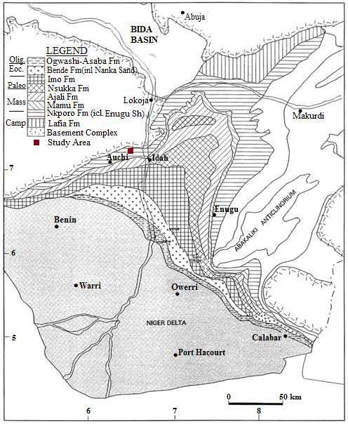
4.1 Crossplot of µ against K
A crossplot of the estimated µ- against estimated K-factor values shows an inverse linear relationship
between the parameters. A correlation coefficient of 0.66 is obtained and shows the extent to which the
estimated soil rigidity and estimated erodibility are linearly related. The correlation would be expected to
increase with carefully measured rigidity and erodibility samples thus leading to a more robust value of λ
for the basin.
20Nwankwo & Okoli ….. Int. J. Innovative Environ. Studies Res. 9(2):11-24, 2021
Fig 2: Plot of Estimated Rigidity against Estimated Erodibility Showing an Inverse Linear
Regression Relationship with a CCF = 0.66 (Source: Graph Plotted with Rigidity and Erodibility
Data Obtained from Table 1.0)
4.2 Computation of Soil Loss Rates Using Our New Geophysical Soil Loss Equation
We have used rigidity data obtained for the Anambra basin area from existing works in the literature
(Atat, et al., 2012; Babatunde, et al., 2016). The mean area constant, λ, for the Anambra basin area was
earlier obtained as 2.438 x 10¹² t2ha-1hr-1MJ-1 (Table 1). λ however varies from one
geographical/geological region to another and must be carefully determined for a given geographically
delineated area or region. The λ-value in conjunction with the rigidity data has been used as input in our
new geophysically modified equation to compute the soil loss rates (Table 2).
Table 2: Results on Soil Loss Rates Obtained from Input of Estimated λ-, μ- and other Values into
Our New Geophysical Model
Area µ-value R-value LS-value C-value P-value Annual
Covered (tmmhr-2ha-1) (MJmmha- Soil Loss
(Km2) ( x1017) 1 -1 -1
hr yr ) (tha-1yr-1)
114.75 65.3 4510.0 39.5 1.0 1.0 0.06651
92.28 79.2 4510.0 39.5 1.0 1.0 0.05483
1348.5 181.9 4510.0 39.5 1.0 1.0 0.02387
621.55 292.1 4510.0 39.5 1.0 1.0 0.01487
11.26 342.0 4510.0 39.5 1.0 1.0 0.01270
From Table 2, for the entire area, the fixed value of erosivity used in our new equation is 4510.0
MJmmha-1hr-1yr-1 and the fixed value of LS-factor used is 39.5. Estimated rigidity values used are 6.53 x
1018, 7.92 x10¹⁸, 1.819 x 10¹⁹, 2.921 x10¹⁹, and 3.420 x 10¹⁹ tmmhr-2ha-1, yielding soil loss rates of
0.06651, 0.05483, 0.02387, 0.01487, and 0.01270 tha-1yr-1 respectively. The erosion in the area is
observed to be slight considering the soil loss rates. The soil loss rate or erosion can also be observed to
21Nwankwo & Okoli ….. Int. J. Innovative Environ. Studies Res. 9(2):11-24, 2021
decrease with increase in rigidity. These results show that whenever rigidity data are available which can
be acquired directly from seismic refraction method of measurement, determination or prediction of
gullying in Anambra basin and its environs can be achieved using our new Geophysical Soil Loss
Equation. As earlier emphasized, we have used estimated rather than actual rigidity data and fixed values
of erosivity and LS-factor in the calculations. The results obtained with our new model can therefore be
improved with field measurements that yield actual rather than estimated values.
5.0 DISCUSSION
The familiar universal soil loss equation is given by A = R x K x L x S x C x P with the parameters
retaining their usual meanings. Our new geophysically modified soil loss equation is given by
A=λxRxLxSxCxP.
µ
This equation excludes the erodibility factor K but allows the input of the rigidity or shear modulus μ (an
elastic geophysical parameter). λ represents a proportionality constant which we have for the purpose of
this study called the Area Constant. The essence of replacing ‘erodibility factor’ with ‘rigidity modulus’ is
hinged on the fact that erodibility is relatively difficult to measure and its evaluation in any soil erosion
prediction modeling requires some rigorous process that is prone to error. The results obtained using our
new geophysical model compare favourably and are quite in agreement with the results obtained in the
literature using the conventional prediction models. Our analysis results show that only slight soil erosion
is occurring in the study area with values of annual soil rates lying between 0.013 and 0.067 tha-1yr-1
compared with the slight erosion rates of 0 - 10 tha-1yr-1 obtained by Babatunde et al, 2016 in the same
study area. Our results are therefore reasonably consistent with results in the literature in spite of using
estimated μ- and λ-values. There is no doubt that as rigidity and area constant (as well as erosivity and the
LS-values) used in our new model approach more accurate values than estimated values, results obtained
become more robust using the new model. Besides, as documented in the literature, increase in erodibility
generally initiates increase in soil loss rates (Igwe et al, 1995; Hughes and Prosser, 2012; Babatunde et al,
2016). This scenario is consistent with the results obtained with our new geophysical model since
decrease in rigidity results in increase in soil loss rates. The rigidity term is an inverse of the erodibility
factor. For example, with rigidity values of 6.53 x 10¹⁸, 7.92 x10¹⁸, 1.819 x 10¹⁹, 2.921 x10¹⁹, and 3420 x
1019 tmmhr-2ha-1, we obtained soil loss rates of 0.06651, 0.05483, 0.02387, 0.01487,and 0.01270 tha-1yr-1
respectively, thus depicting decrease in soil loss rates with increase in rigidity. These results obtained
show that availability of accurate input data is all that is needed to obtain reliable results with our new
model. To make λ and μ robust for use in the new model therefore requires field measurements that yield
actual rather than estimated values. Solving this problem should serve as an extension of this work by
future researchers. The work can also be extended to determine the area constant, λ, for the entire
Southeast of Nigeria using measured rather than estimated data.
6.0 CONCLUSION
We have successfully modified the universal soil loss equation by substituting the soil erodibility factor
with the rigidity factor – an elastic geophysical parameter. Since conventional methods of soil erosion
prediction incorporate the term – the erodibilty factor - which is inherently difficult to measure and error-
prone, we have decently eliminated this inherent problem by introducing a new term – the rigidity factor-
in our new model which can achieve accurate and robust prediction results without loss of generality and
computational speed. We have also introduced a new constant into our new equation called the area
constant. We however admonish that the new constant is uniquely characteristic of any given
geographical/geological region, implying that the constant must be carefully determined for a given
geographical/geological region before it can be used for computation of soil loss rates. In the final
analysis, we are confident that we have successfully derived a new soil loss equation suitable for erosion
prediction, monitoring and control in any part of the world. However, we do not claim to have exhausted
22Nwankwo & Okoli ….. Int. J. Innovative Environ. Studies Res. 9(2):11-24, 2021
this approach and hope that more work by future researchers can be extended to this area in order to apply
our model on a larger and more regional scale.
ACKNOWLEDGEMENTS
The authors wish to thank the Vice Chancellor, Prof. T.O. Olagbemiro and Dean of Faculty of Science,
Prof. S.C.O. Ugbolue, both of Edwin Clark University, Delta State, Nigeria, for providing the resources
that facilitated this research. Also big thanks to the authors whose papers we consulted that helped to clear
away many technical hitches during the study. Also, special thanks to Dr. Efosa Edionwe of the
Department of Mathematical Sciences, Edwin Clark University, Delta State, Nigeria, for his
contributions.
REFERENCES
Akpokodje EG, Akaha CT, Ekeocha N (2010). Gully Erosion Geohazards in Southeastern Nigeria and
Management Implications. Scientia Africana 9: 20-36
Alabameri A, Cerda A, Tiefenbacher JP (2019). Spatial Pattern Analysis and Prediction of Gully Erosion
Using Novel Hybrid Model of Entropy-Weight of Evidence. Water 11, 1129: 1-23
Atat JG, Akpabio GT, George NJ, Umoreu EB (2012). Geophysical Assessment of Elastic Constants of
Top Soil Using Seismic Refraction Compressional and Shear Wave Velocities in the Eastern
Niger Delta, Nigeria. International Journal of Modern Applied Physics 1(2): 7-12
Babatunde J F, Adeleye Y B, Chris O, Olabanji OA, Adegoke IA (2016). GIS-based Estimation of Soil
Erosion Rates and Identification of Critical Areas in Anambra Sub-basin, Nigeria. Model Earth
Syst. Environ. 2-159
Berry J, Houston K (1995). Mathematical Modelling: Modular Mathematical Series: Edward Arnold,
London 1-123
Bullen KE, Bruce AB (1993). An Introduction to the Theory of Seismology, 4th Edition.
De Jong SM (1994). Applications of Reflective Remote Sensing for Land Degradation Studies in a
Mediterranean Environment. Nederlandse Geografische Studies 177
De Jong S M, Brouwer LC, Riezebos HT (1998): Erosion Hazard Assessment in the Peyne Catchment,
France. Working Paper DeMon-2 Project. Dept. of Physical Geography, Utrecht University
Egwuonwu CC, Okereke NAA, Ezeanya NC (2013). Characterization of Erodibility Using Soil
Strength and Stress-Strain Indices for Soils in Some Selected Sites in Anambra State. Journal of
Emerging Trends in Engineering and Applied Sciences (JETEAS) 4(2): 333-340
Gideon YB, Fatoye FB, Omad J I (2014). Sedimentological Characteristics and Geochemistry of Ajali
Sandstone Exposed at Ofe-Jiji and Environs Northern Anambra Basin. Nigeria Res J Environ
Earth Sci 6(1): 10-17
Grant FS, West GF (1965). Interpretation Theory in Applied Geophysics, New York: McGraw-Hill,
PP583
Hudec PP, Simpson F. Akpokodje EG, Umenweke M (2005). Anthropogenic Contributions to Gully
Initiation and Propagation, SE Nigeria,, In: Ehlen J, Haneberg WLRA (ed) Humans as Geologic
Agents. Geologic Society of American Reviews in Engineering Geology, XVI, Geologic Society
of America, Boulder, Colorado 149-158
Hudson NW (1981). Soil Conservation. Cornell University Press, New York
Hughes A O and Prosser I P (2012). Gully Erosion Prediction across a Large Region: Murray-Darling
Basin, Australia. Soil Research, 50: 267 – 277
Igwe C A (2005). Erodibility in Relation to Water-Dispersible Clay for Some Soils of Eastern Nigeria.
Land Degradation and Development 16: 87-96.
Igwe CA, Akamigbo F.O, Mbaukwu JSC (1995). The Use of Some Soil Aggregate Indices to Assess
Potential Soil Loss in Soils of Southeastern Nigeria. International Agrophysics, 9: 95-100
23Nwankwo & Okoli ….. Int. J. Innovative Environ. Studies Res. 9(2):11-24, 2021
Jäger S (1994). Modelling Regional Soil Erosion Susceptibility Using the Universal Soil Loss Equation
and GIS. In: Rickson, RJ (ed). Conserving Soil Resources. European Perspectives CAB
International 161-177.
Kirkby MJ, King D (1998). Summary Report on Provisional RDI Erosion Risk Map for France. Report on
Contract to the European Soil Bureau (Unpublished)
Lai R (1976b). Soil Erosion on Alfisols in Western Nigeria; Effects of Rainfall Characteristics. Geoderma
16: 389- 401
Morgan RPC (1992). Soil Erosion in the Northern Countries of the European Community. EIW
Workshop. Elaboration of a Framework of a Code of Good Agricultural Practices, Brussels, 21-
22
Morgan RPC, Morgan DDV, Finney HJ (1984). A Predictive Model for the Assessment of Soil Erosion
Risk. Journal of Agricultural Engineering Research 30: 245-253.
Nwabuokei PO (2001). Fundamentals of Statistics. Korunna Books, Enugu, Nigeria 289-337
Nwajide CS (1990). Cretaceous Sedimentation and Palaeogeography of Central Benue Trough, in:
Ofoegbu CO (ed) the Benue Trough Structure and Evolution. Friedr.Viewed and
Sohn,Braunhweig/Wiesbaden 19- 38
Oboh-Ikuenobe FE, Obi CG, Jaramillo CA (2005). Lithofacies, Palinofacies, and Sequence Stratigraphy
of Palaeogene Strata in Southeastern Nigeria. J. Afri Earth Sc 41: 79-101
Ofomata GEK (1981). Actual and Potential Erosion in Nigeria and Measures for Control. Soil Science
Society of Nigeria Special Nomograph 1: 151-165
Ofomata GEK (1985) Soil Erosion, Southeastern Nigeria: the View of a Geomorphologist. Inaugural
Lecture Series, University of Nigeria Nsukka
Oldeman LR, Hakkeling RTA, Sombroek WG (1991). World Map of the Status of Human-Induced Soil
Degradation, with Explanatory Note (Second Revised Edition). ISRIC, Wageningen UNEP,
Nairobi.
Onwuka SU, Okoye CO, Nwagbo N (2012). The Place of Soil Characteristics on Soil Erosion in Nanka
and Ekwuobia Communities in Anambra State. J Environ Manag Safety 3(3): 31-50
Reyment RA (1965). Aspect of the Geology of Nigeria. University of Ibadan Press, Nigeria
Romkems MJM, Young RA, Poesen JWA, McCool DK, El-Swaify SA, Bradford J M (1997). Soil
Erodibility Factor in: Foster GR, Weesies GA., McCool DK., Yoder DC (eds), Predicting Soil
Erosion by Water: a Guide to Conservation Planning with the Revised Universal Soil Loss
Equation (RUSLE). Agriculture Handbook Washington DC, USA: US Department of
Agriculture, Agricultural Research Service (703): 65-69.
Stocking MAA (1987). Methodology for Erosion Hazards Mapping of the SADCC Region. Paper
Presented at the Workshop on Erosion Hazard Mapping, Lusaka, Zambia
Van Lynden GWJ (1995). European Soil Resources. Nature and Environment, Council of Europe,
Strasbourg (71)
Wischmeier WH, Smith DD (1978). Predicting Rainfall Erosion Losses – a Guide for Conservation
Planning. U.S. Department of Agriculture, Agriculture Handbook 537
Wischmeier WH, Johnson CB (1971). Soil Erodibility Nomograph for Farmlands and Construction Sites.
J Soil Water Conserv 26(5): 189-193
24You can also read