Feature Extraction for Content-Based Image Retrieval Using a Pre-Trained Deep Convolutional Neural Network
←
→
Page content transcription
If your browser does not render page correctly, please read the page content below
DEGREE PROJECT IN COMPUTER SCIENCE AND ENGINEERING,
SECOND CYCLE, 30 CREDITS
STOCKHOLM, SWEDEN 2020

Feature Extraction for Content-
Based Image Retrieval Using a Pre-
Trained Deep Convolutional Neural
Network

LEONARD HALLING

KTH ROYAL INSTITUTE OF TECHNOLOGY
SCHOOL OF ELECTRICAL ENGINEERING AND COMPUTER SCIENCE

Author

Leonard Halling
leonardh@kth.se
Master’s program in Computer Science
KTH Royal Institute of Technology

Place for Project

Monok AB
Stockholm, Sweden

Examiner

Jonas Beskow
KTH Royal Institute of Technology
Stockholm, Sweden

Supervisor

Hamid Reza Faragardi
KTH Royal Institute of Technology
Stockholm, Sweden

2020-04-08

Abstract
This thesis examines the performance of features, extracted from a pre-trained
deep convolutional neural network, for content-based image retrieval in im-
ages of news articles. The industry constantly awaits improved methods for
image retrieval, including the company hosting this research project, who
are looking to improve their existing image description-based method for
image retrieval. It has been shown that in a neural network, the invoked ac-
tivations from an image can be used as a high-level representation (feature)
of the image. This study explores the efficiency of these features in an image
similarity setting. An experiment is performed, evaluating the performance
through a comparison of the answers in an image similarity survey, contain-
ing solutions made by humans. The new model scores 72.5% on the survey,
and outperforms the existing image description-based method which only
achieved a score of 37.5%. Discussions about the results, design choices, and
suggestions for further improvements of the implementation are presented
in the later parts of the thesis.

                                     1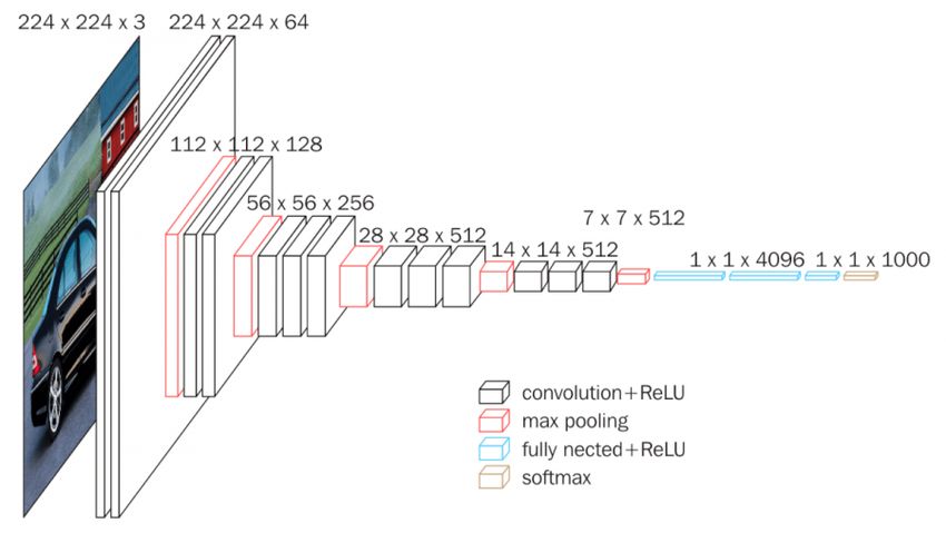
Sammanfattning
Detta examensarbete utforskar huruvida representationer som extraherats
ur en förtränad djup CNN kan användas i innehållsbaserad bildhämtning för
bilder i nyhetsartiklar. Branschen letar ständigt efter förbättrade metoder
för bildhämtning, inte minst företaget som detta forskningsprojekt har ut-
förts på, som vill förbättra sin befintliga bildbeskrivningsbaserade metod
för bildhämtning. Det har visats att aktiveringarna från en bild i ett neuralt
nätverk kan användas som en beskrivning av bildens visuella innehåll (fea-
tures). Denna studie undersöker användbarheten av dessa features i ett bild-
likhetssammanhang. Ett experiment med syfte att utvärdera den nya mod-
ellens prestanda utförs genom en jämförelse av svaren i en bildlikhetsunder-
sökning, innehållande lösningar gjorda av människor. Den nya modellen får
72,5% på undersökningen, vilket överträffar den existerande bildbeskrivn-
ingsbaserade metoden som bara uppnådde ett resultat på 37,5%. Diskus-
sioner om resultat, designval samt förslag till ytterligare förbättringar av ut-
förandet presenteras i de senare delarna av rapporten.

                                       2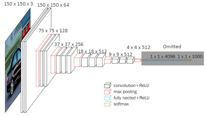
Contents
1   Introduction                                                                                                          5
    1.1 Background . . . . . . . .    .   .   .   .   .   .   .   .   .   .   .   .   .   .   .   .   .   .   .   .   .   5
        1.1.1 Monok Dataset . .       .   .   .   .   .   .   .   .   .   .   .   .   .   .   .   .   .   .   .   .   .   5
        1.1.2 Current Algorithm       .   .   .   .   .   .   .   .   .   .   .   .   .   .   .   .   .   .   .   .   .   6
    1.2 Objective . . . . . . . . .   .   .   .   .   .   .   .   .   .   .   .   .   .   .   .   .   .   .   .   .   .   6
    1.3 Research Question . . . .     .   .   .   .   .   .   .   .   .   .   .   .   .   .   .   .   .   .   .   .   .   6
    1.4 Research Methodology .        .   .   .   .   .   .   .   .   .   .   .   .   .   .   .   .   .   .   .   .   .   7
    1.5 Scope and Limitations . .     .   .   .   .   .   .   .   .   .   .   .   .   .   .   .   .   .   .   .   .   .   8
    1.6 Structure of the Report .     .   .   .   .   .   .   .   .   .   .   .   .   .   .   .   .   .   .   .   .   .   8

2 Background                                                                                                               9
  2.1 Supervised Learning . . . . . . . . . . . . .                           .   .   .   .   .   .   .   .   .   .   .    9
      2.1.1 Stochastic Gradient Descent (SGD)                                 .   .   .   .   .   .   .   .   .   .   .    9
      2.1.2 Backpropagation . . . . . . . . . . .                             .   .   .   .   .   .   .   .   .   .   .    9
  2.2 Convolutional Neural Networks . . . . . .                               .   .   .   .   .   .   .   .   .   .   .   10
      2.2.1 Convolutional Layer . . . . . . . . .                             .   .   .   .   .   .   .   .   .   .   .   10
      2.2.2 Pooling Layer . . . . . . . . . . . .                             .   .   .   .   .   .   .   .   .   .   .   11
      2.2.3 ReLU Layer . . . . . . . . . . . . . .                            .   .   .   .   .   .   .   .   .   .   .   12
      2.2.4 Fully-Connected Layer . . . . . . .                               .   .   .   .   .   .   .   .   .   .   .   12
      2.2.5 Loss Layer (Softmax) . . . . . . . .                              .   .   .   .   .   .   .   .   .   .   .   12
  2.3 Transfer Learning . . . . . . . . . . . . . .                           .   .   .   .   .   .   .   .   .   .   .   13
  2.4 Distance Metric Learning . . . . . . . . . .                            .   .   .   .   .   .   .   .   .   .   .   13
      2.4.1 Siamese/Triplet Networks . . . . .                                .   .   .   .   .   .   .   .   .   .   .   13

3 Related Works                                                        15
  3.1 CNN-based approaches . . . . . . . . . . . . . . . . . . . . . . 15
  3.2 Conventional Image Retrieval . . . . . . . . . . . . . . . . . . 17

4 Method                                                                                                                  18
  4.1 Network Architecture and Configurations                             .   .   .   .   .   .   .   .   .   .   .   .   18
      4.1.1 ImageNet Classification . . . . . .                           .   .   .   .   .   .   .   .   .   .   .   .   18
      4.1.2 Feature Extraction . . . . . . . . .                          .   .   .   .   .   .   .   .   .   .   .   .   19
  4.2 Data Pre-processing . . . . . . . . . . . .                         .   .   .   .   .   .   .   .   .   .   .   .   19
  4.3 Similarity Evaluation . . . . . . . . . . .                         .   .   .   .   .   .   .   .   .   .   .   .   24
  4.4 Experiment . . . . . . . . . . . . . . . . .                        .   .   .   .   .   .   .   .   .   .   .   .   24
  4.5 Tools Used . . . . . . . . . . . . . . . . .                        .   .   .   .   .   .   .   .   .   .   .   .   25

                                          3
5 Results                                                                                                                     26
  5.1 Experiment . . . . .    .   .   .   .   .   .   .   .   .   .   .   .   .   .   .   .   .   .   .   .   .   .   .   .   26
  5.2 Desirable Results . .   .   .   .   .   .   .   .   .   .   .   .   .   .   .   .   .   .   .   .   .   .   .   .   .   26
  5.3 Undesirable Results     .   .   .   .   .   .   .   .   .   .   .   .   .   .   .   .   .   .   .   .   .   .   .   .   26
  5.4 Unusable Results . .    .   .   .   .   .   .   .   .   .   .   .   .   .   .   .   .   .   .   .   .   .   .   .   .   30

6 Discussion                                                                                                                  32
  6.1 Validity of the Results . . . . .               .   .   .   .   .   .   .   .   .   .   .   .   .   .   .   .   .   .   33
      6.1.1 Sample Size . . . . . . .                 .   .   .   .   .   .   .   .   .   .   .   .   .   .   .   .   .   .   33
      6.1.2 Definition of Similarity                  .   .   .   .   .   .   .   .   .   .   .   .   .   .   .   .   .   .   33
  6.2 Future Work . . . . . . . . . .                 .   .   .   .   .   .   .   .   .   .   .   .   .   .   .   .   .   .   34
  6.3 Ethical Aspects . . . . . . . . .               .   .   .   .   .   .   .   .   .   .   .   .   .   .   .   .   .   .   34

                                              4
1    Introduction
1.1 Background
Learning similarities between pairs of images is an essential problem in com-
puter vision. Its usefulness can be seen in many different applications, such
as image search, facial recognition, and similar image ranking.

Monok AB provides a platform which automatically scrapes, analyzes and
clusters online news articles. A cluster for an article consists of a summary,
several news sources, source images, along with keywords, mentions etc.
Several companies such as Monok AB that hosted this research project are
now developing a model for automatic text-generation where news clusters/sum-
maries are written for both consumers and journalists alike. Furthermore,
they are looking for a new approach of retrieving a suitable image for each
news cluster. The retrieved image should preferably be as similar as possible
to any of the images of the source articles. The first part of the image retrieval
process is to search several online repositories of free-use query images such
as Wikimedia Commons, Flickr etc. However, this part is not focused on in
this thesis. Instead, this thesis targets the image similarity ranking, given a
retrieved set of query images and a set of source images. The outputs are the
query images most similar to any of the source images.

1.1.1 Monok Dataset
The dataset provided from Monok, the host company, contains every news
cluster generated for the past two years, as well as the original articles that
make up the clusters. Since this thesis focuses on image similarity, a lot of
information in the dataset can be discarded, such as people mentions, loca-
tions and keywords. The images included in the dataset exists both as full
images, but also as cropped, 150 x 150 pixels thumbnails. For each news
cluster in the dataset, the images from the source articles are present. For
each news cluster, images from the retrieval process are stored in arrays as
well, sorted by relevance established by the image description-based algo-
rithm.

                                      5
1.1.2 Current Algorithm
The current algorithm is solely based on looking at the image descriptions of
the images. The central part of the current approach is to compute the tf-idf
(term frequency–inverse document frequency) of the descriptions, which is
a metric designed to indicate the importance of words in text [16]. A similar-
ity metric is then computed to estimate the similarity between images. The
host company also has some heuristic requirements for the images, such as
file type, resolution and aspect ratio, which are handled by the algorithm
as well. The image description-based algorithm is currently involved both
in the initial retrieval stage, as well as the image ranking stage. The algo-
rithm returns an array with the query images, sorted by their similarity to
the source images. The performance of the existing algorithm is bearable,
but will often produce results that are not satisfactory to the host company.
One considerable issue with the current approach is that images without de-
scriptions have to be disregarded, which is a problem that could be avoided
by implementing an algorithm that compares the semantic similarity of the
actual images.
1.2 Objective
The objective of this thesis is to investigate the use of deep learning in content-
based image retrieval, and to perform experiments to test the performance
of the new algorithm.
The main objective of the thesis is to suggest an applicable architectural and
technical solution for the problem as described above, and to compare its
performance to the image description-based method. The description-based
method is still involved in retrieving the initial set of query images from the
web, and this thesis aims to improve the similarity ranking of the already
retrieved set of images.
1.3 Research Question
There are two questions that will be answered in this thesis:
How can the CNN from [21] be implemented and trained for the task of
content-based image retrieval?
6Can the features of the pre-trained model be used to outperform the im-
age description-based method in the specific task of content-based image
retrieval in a new setting, on a different dataset consisting of news articles?
1.4 Research Methodology
In Figure 1.1, the research methodology used in this thesis is shown. Af-
ter the first three steps, there is an iterative process including researching
feasible approaches, implementing said approach, and evaluating the im-
plementation to conclude the performance of the model and if the approach
was suitable for the problem.
Figure 1.1: Research methodology
71.5 Scope and Limitations
This thesis does not focus on the image retrieval process, that is, the process
of how the query images are retrieved, and the pros and cons of using various
free-use repositories online.
While it would be interesting to explore the performance of a combination
between the results of the neural network model and the current approach,
this task is also considered out of the scope of this thesis, and is instead a
suggestion for future work.
1.6 Structure of the Report
The thesis is divided into the following sections:
• Section 2 - Background provides the necessary knowledge as a foun-
dation for the thesis.
• Section 3 - Related Works introduces relevant related works that have
been done in the field, and discusses some of the different approaches
that have been studied.
• Section 4 - Method describes how the method to address the research
problems has been carried out and what experiments have been done.
• Section 5 - Results presents the results of the experiments conducted.
• Section 6 - Discussion aims to analyze and understand the results and
addresses their significance. A discussion about the validity of the re-
sults is included, as well as recommendations for future work and eth-
ical aspects.
82 Background
2.1 Supervised Learning
Supervised learning is the procedure of learning a function that maps a given
input x, to an output y, based on a set of training examples. Equivalently,
given a training set of input-output pairs
(x1 , y1 ), (x2 , y2 ), ...(xN , yN )
where each yj was generated by an unknown function y = f (x), we want to
find a function h that approximates the true function f [19]. A loss func-
tion is defined in order to make it into an optimization problem. A loss
function maps the values of several variables of an event into one real num-
ber that represents some cost associated to the event. One can optimize the
problem by minimizing the loss function.
2.1.1 Stochastic Gradient Descent (SGD)
Stochastic gradient descent, or SGD, is an iterative method of minimizing a
loss function. Consider the sum of squared errors loss function E and weight
vector w:
1X
E(w) = (targeti outputi )2 . (1)
2 i
The weight update is computed by taking a step in the opposite direction of
the gradient of the loss function. Thus, the new weight vector becomes
wnew = w ⌘ E(w) (2)
where ⌘ is the step length or the learning rate. This update is repeated by iter-
ating through the data. When combining SGD with the backpropagation
algorithm, it is the standard algorithm for training artificial neural networks
[3, 11].
2.1.2 Backpropagation
Backpropagation, or backprop, is a technique for evaluating the gradient of
an error function for a feed-forward neural network. This is achieved by
calculating an error at the output layer of a network and distributing it back-
wards throughout the network.
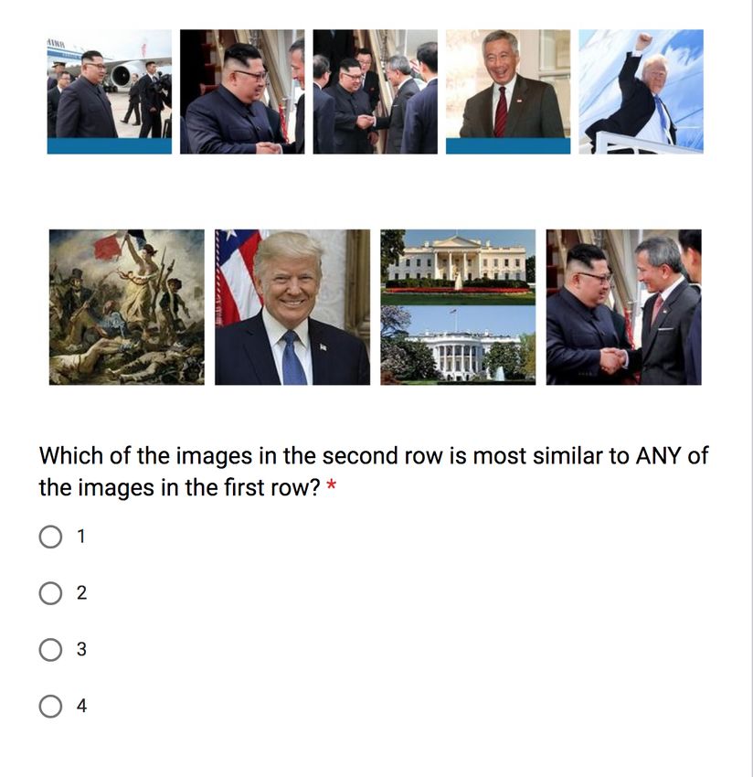
9Figure 2.1: The activation maps in a simple convolutional neural network
with architecture [conv-relu-conv-relu-pool]x3-fc-softmax. The last layer
stores the scores for each class. [14]
2.2 Convolutional Neural Networks
A convolutional neural network (CNN), is a deep neural network suitable
for visual imagery. Similarly to regular neural networks, they consist of an
input layer, multiple hidden layers, and an output layer. Typically, the hid-
den layers consists of convolutional layers, ReLU layers, pooling layers, and
fully-connected layers [14].
2.2.1 Convolutional Layer
The convolution layer is the core building block of a CNN. It consists of a
set of filters. A filter can be seen as a smaller window that convolves (slides)
across the input image and computes dot products between the values of the
filter and the pixel values of the input image. The output of this action is a
2-dimensional activation map that shows the responses of the filter at each
position. Each convolutional layer has a set of filters, and each filter will
produce a separate 2-dimensional map. These separate activation maps are
stacked to produce the output of the convolutional layer. Figure 2.1 shows
the activation maps in an example CNN architecture.
The width and height of the filters are hyper-parameters, while the depth
of the filters must be equal to the depth of the input image. Other hyper-
10parameters that are to be considered, which all will affect the size of the out-
put image, are:
• Number of filters. This will affect the number of stacked activation
maps in the output of the layer.
• Stride. The stride specifies how many steps at the time the filter will
move across the image. When the stride is set to 2 or more, the filter
would jump 2 or more pixels at a time which would produce an output
with smaller width and height than the input.
• Zero-padding pads the input image with zeros around its border.
Most commonly, zero-padding is used to preserve the size of the in-
put size to the output.
It is now somewhat simple to see how these hyper-parameters affect the size
of the output. For example, if we have an input image of size 10 x 10 and
a filter of size 3 x 3 with stride 1 and zero-padding = 0, we would get an
output image of size 8 x 8. If we would like to preserve the size, we would set
zero-padding to be 1, and the output would result in a size of 10 x 10. Notice
that we wouldn’t be able to set the stride to 2 with zero-padding = 0 in this
example, since the filter wouldn’t fit evenly in the image. The stride must be
set such that the filter could slide neatly across the image [14].
2.2.2 Pooling Layer
The purpose of the pooling layer is to reduce the number of parameters and
computation in the network by reducing the spatial size of the image repre-
sentations. The most commonly applied type of pooling is max-pooling. A
max-pooling layer with a filter size of 2 x 2 and stride 2, moves across the
input image and utilizes the MAX operation at every step. Since the filter is
taking the max over 4 numbers, the action removes 3/4 of the information.
There are two commonly seen settings of the max-pooling layer: Size = 2 x 2
with stride = 2, and size = 3 x 3 with stride = 2. The second setting is called
overlapping pooling and was one of the contributions of [10], a study which
will be discussed later in this paper.
112.2.3 ReLU Layer
The convolutional layers are often followed by Rectified Linear Unit (ReLU)
layers, which applies the activation function
f (x) = max(0, x) (3)
to the input x. This increases the non-linearity of the network while also
removing negative values from the activation maps. Traditionally, other
function were used such as f (x) = tanh(x) or the sigmoid function f (x) =
(1 + e 1 ) 1 , but the ReLU function has shown to be faster and is generally
preferred [10, 17].
2.2.4 Fully-Connected Layer
Much like traditional multi-layer perceptrons, the neurons in the fully con-
nected layers have complete connections to all activations in the previous
layer. Note that a convolutional layer can be seen as a fully-connected layer
with neurons being the filters, only that the neurons in the convolutional
layers are connected to a local region in the input image, and many of the
neurons in the convolutional layer share parameters [14]. It has been shown
that it is possible to remove the fully connected layers from a CNN while still
achieving good performance, by using the output from the convolutional and
pooling layers [2]. This approach will be explored in this study by ommitting
the fully-connected layers and using the output from the last max-pooling
layer as feature vectors for each image.
2.2.5 Loss Layer (Softmax)
The loss layer is usually the last layer of the neural network. The purpose
of the loss layer is to specify penalty between the prediction and the true
label (target) during training. For classification, the softmax is used. The
softmax layer takes the previous layer as input, and produces a probability
distribution of K probabilities as output, where K is the number of classes
during training. The output from the softmax layer is used to compute a loss
which can then be back-propagated through the network [3].
122.3 Transfer Learning
Obtaining large, annotated datasets like ImageNet [12] for a specific domain
can be challenging. One approach one can take to circumvent this challenge
is transfer learning. Transfer learning in machine learning focuses on the
problem of transferring knowledge learned from one task, and applying it
to solve a different related task [26]. In this case, a convolutional neural
network, pre-trained for classification on the ImageNet dataset, is used for
feature extraction of images unrelated to the dataset used for training.
2.4 Distance Metric Learning
In metric learning, we want to find a function that maps input patterns to
an output space, where a distance can be computed to approximate the sim-
ilarity in the input space [4].
2.4.1 Siamese/Triplet Networks
The Siamese network is an architecture comprised of 2 instances of the
same same feed-forward network with shared parameters. The network is
learning similarity metrics, by training the network on pairs of images. Both
[4] and [8] employs the Siamese network, where a contrastive loss based on
the similarity metric is used to train the network to characterize pairs of im-
ages to be similar or dissimilar. The constrastive loss aim to ensure that
similar pairs gets a small distance, and that a large distance is given to dis-
similar pairs. [9] discusses the issues with the approach of pairwise training.
According to the authors, the main issue with the Siamese networks is that
they are “sensitive to calibration in the sense that the notion of similarity
vs dissimilarity requires context”. For example, one person could be con-
sidered similar to another person when learning on a dataset with random
objects. But in another context, where we would like to distinguish persons
in a set of individuals only, the same two persons might be determined dis-
similar. The issue of calibration is not needed in Triplet networks, and [9]
argues that the Triplet network outperforms the Siamese network in metric
learning for classification.
The Triplet network consists of 3 instances of the same feed-forward net-
work. The network takes image triplets as input. An image triplet consists
of a query image, a positive image (more similar to the query image), and
13a negative image (more dissimilar to the query image). Instead of the con-
trastive loss as in the Siamese network, the loss is based on the two distances
between the query image and the positive/negative image in the output, and
is back-propagated through the network, updating the parameters via SGD
[9, 25].
143 Related Works
This paper lies in the area of image similarity with deep neural networks.
In this following section, several existing approaches in image similarity are
presented and discussed.
3.1 CNN-based approaches
AlexNet [10], won the ILSVRC (ImageNet Large Scale Visual Recognition
Competition) [18] 2012 by a long shot, scoring an error rate of 15.3% with
the runner up scoring 26.2% [10]. The success of [10] has been a great inspi-
ration for the use of convolutional neural networks in image recognition. A
selection of the main contributions from the authors are the use of Rectified
Linear Units nonlinearity (ReLU) as the activation function, i.e the neurons
output f as a function of its input x with
f (x) = max(0, x) (4)
as opposed to the standard way up until then, which was
f (x) = tanh(x) (5)
or
f (x) = (1 + e x ) 1
(6)
Another big contribution of [10] was the use of Dropout instead of regular-
ization. Dropout consists of setting the output of a neuron to zero with a
probability of 0.5, in order to prevent overfitting. The complexity of the net-
work entails expensive training, especially considering the magnitude of the
ImageNet dataset. The authors have tackled this problem by developing an
optimized GPU implementation utilized when training the network.
Neural Codes for Image Retrieval [2], has done a similar study to this
one where they are using neural codes extracted from a reimplementation
of the system from [10]. This study was heavily inspired by the findings
of [2] since it showed that neural codes from the pre-trained convolutional
neural network would perform well on related image retrieval tasks. In [2],
the performance of neural codes from three different layers were examined.
Compressed neural codes, where Principal Component Analysis (PCA) were
15utilized to achieve shorter codes, was also shown to result in very good per-
formance. This finding, while interesting, is not essential to the purpose of
this study since the images are sampled and the features are extracted in an
online fashion rather than stored in a database. Furthermore, the CNN im-
plementation that [2] is based on has been surpassed since, and one of the
aims of this study is to explore the performance of feature vectors extracted
from an improved CNN implementation.
VGGNet [21], invented by The Visual Geometry Group (VGG), achieved
very good performance on the ImageNet dataset, being the first runner up in
the ILSVRC 2014 in the classification task. The authors main contribution is
implementing a CNN using very small (3 x 3 pixel) convolution filters while
pushing the depth of the network to 16 layers, which allows for a consistant
architecture throughout the network. This study is utilizing the CNN from
[21] as the pre-trained network for extracting feature vectors, partly because
of its great success on the ILSVRC 2014, but also because the authors have
made the architecture and the weights of the trained network freely available
online.
Deep Ranking [25], uses the CNN implementation in [10] to propose a
deep ranking model for fine-grained image similarity learning. The model
is using a triplet network to outline the fine-grained relationships in images.
Although triplet sampling were not implemented in this study, it’s advan-
tages will be discussed under the section Future Work.
[23] propose R-MAC, a method of feature extractions in regions in an image.
Using regions adds recognition of the location of the features in the image,
which, according to the authors offers significantly better performance than
directly extracting features from the full image. [7] propose an extension
of the R-MAC by (1) introducing a triplet network, optimizing the R-MAC
weights for the image retrieval task, and (2) introducing region proposals, a
learning mechanism for predicting the regions of interest in an image instead
of the rigid grid of the original R-MAC. It is shown that the region propos-
als significantly outperform the rigid grid. While implementing the region
proposals would be out of the scope of this project, the idea is nevertheless
interesting and could be utilized in the pre-processing stage of this project
as an alternative to smart cropping of the images.
163.2 Conventional Image Retrieval
The conventional image retrieval techniques are based on bag of visual words
(BOVW) [22], which is the idea of constructing vocabularies by extracting
features in images. Images could then be represented as a frequency his-
togram of features, which is used to predict the class of the image or to find
similar images. [13] proposes an extension of BOVW by using a vocabulary
tree, which allows more efficient lookup of visual words and is shown to in-
crease the retrieval quality. [15] uses spatial verification to further improve
the image ranking performance. One of the main advantages in using neu-
ral networks is that the features are data-driven while, when using one of the
conventional techniques, the features are hand-crafted.
174 Method
In this section, the process of using a pre-trained convolutional neural net-
work for feature extraction is described. Substantial work has also been done
on the Monok dataset, and issues regarding image retrieval, cropping, and
resizing that have arisen will be discussed as well.
4.1 Network Architecture and Configurations
4.1.1 ImageNet Classification
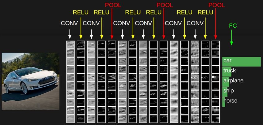
Figure 4.1 visualizes the outline of the network architecture, the design is
heavily inspired by configuration D in [21]. Configurations D (16 layers)
and E (19 layers) performed the best in the experiments in [21], and D was
selected for this project since it has fewer layers which facilitates the im-
plementation. When training the CNN on classification of the ImageNet
dataset, RGB images of size 224 x 224 are used as input. A bit of pre-processing
is done by subtracting the mean RGB value of the training set from each
pixel in the image. The model consists of a stack of convolutional layers,
all of them using filters with a small receptive field of size 3 x 3 pixels. The
stride is set to 1 pixel, and the spatial padding is 1 pixel as well to preserve the
spatial resolution after convolution. Some convolutional layers are followed
by max-pooling layers. Throughout the network there are five max-pooling
layers where pooling is performed over a 2 x 2 pixel window using stride 2.
After the last max-pooling layer, three fully-connected layers are introduced.
The first two have 4096 channels each, while the third layer performs the
classification and has 1000 channels, one for each class. The softmax layer
comes last. The rectification non-linearity (ReLU) is applied to both the con-
volutional and the fully-connected layers.
The procedure for training the CNN in [21] largely follows [10]. The batch
size was set to 256, with momentum 0.9. Weight decay was used to reg-
ularise training with the L2 penalty coefficient set to 5 · 10 4 , and dropout
were utilized for the first two fully-connected layers with the dropout ratio
set to 0.5. The learning rate was initialized to 10 2 , and decreased by a fac-
tor of 10 when the validation accuracy stopped improving. The learning was
stopped after 74 epochs.
184.1.2 Feature Extraction
The concept of transfer learning is to use the weights of the network, learned
during classification, for feature extraction. Figure 4.2 shows the difference
in the network architecture when performing feature extraction. The ma-
jor difference here is that the fully-connected layers, as well as the soft-max
layer, are omitted and that the output of the last max-pooling layer is used
to construct the feature vectors which in turn are used to calculate the dis-
tances between the models representations of the input images. Section 4.3
describes the similarity metrics further.
The input shape has also been altered to support the aspect ratio that is al-
ready adapted used in the previous system developed by Monok. Altering the
input shape, and therefore the shape of the whole network, after training is
possible since no further classification will be done, only feature extraction.
4.2 Data Pre-processing
The retrieved images that are to be evaluated first have to be resized to 150 x
150 pixels. There are several different approaches for achieving this; smart
cropping to regions of interest, resizing, and simply cropping were the three
options that were explored. Smart cropping entails finding the Regions of
Interest (ROIs) in images, and performing automatic cropping to the most
interesting regions [1]. Although smart cropping at times yielded decent re-
sults, the consistency of the approach couldn’t be guaranteed. Figures 4.3,
4.4 and 4.5 shows selections of images before and after being smart cropped.
Observable in the figures is that as the original images grow in size, the out-
come from the smart cropping gets less ideal. The scope of this project didn’t
allow for further exploration on the topic.
The chosen approach was resizing and cropping from center as needed, which
on average gave useful results. A selection of resized/cropped images can
also be seen in the figures. Furthermore, the mean RGB values were sub-
tracted from each pixel, similarly to [21], in order to center the pixel values
around zero, since the model expects the pixel values to have zero mean.
19Figure 4.1: Model architecture for classification on the ImageNet dataset
(1000 classes). [24]
Figure 4.2: Model architecture for feature extraction on the Monok dataset.
20Figure 4.3: A selection of smart cropped and resized+cropped images, both
with desirable results. The original image to the left, followed the smart
cropped image in the middle and resized+cropped image to the right.
21Figure 4.4: A selection of smart cropped and resized+cropped images. The
original image is on top, with the smart cropped image on the bottom left,
and the resized+cropped image on the bottom right. The bigger the original
images get, the worse the results of the smart cropped images becomes.
22Figure 4.5: A selection of smart cropped and resized+cropped images. The
original image is on top, with the smart cropped image on the bottom left,
and the resized+cropped image on the bottom right. The bigger the origi-
nal images get, the worse the results of the smart cropped images becomes
(cont).
234.3 Similarity Evaluation
The similarity between the feature vectors are measured by first using L2
normalization, and then computing the L2-distance between the vectors.
Following the principals requirements, the program should, for a given news
article:
• Take two sets as input; one set contains the images from the news
sources, the other contains the retrieved query images.
• Return a set of the most similar query images, ranked by their similar-
ity to any of the images in the source set.
The program iterates through every image in the source set and computes
the distance to every image in the query set, ranking the query image that
has the shorter distance to any of the source images higher.
4.4 Experiment
The experiment was divided into two parts. First, a qualitative study was
performed with human test subjects in order to establish a ground truth.
Second, a quantitative study was done where the neural network model and
the image description-based algorithm were compared. 40 clusters contain-
ing a total of 370 images were randomly sampled from the Monok dataset.
The samples were made into questions, each question containing 2-5 query
images and a set of source images.
In the qualitative study, 40 test subjects answered a survey consisting of the
40 questions. The test subjects were asked to determine which of the query
images that they thought was the most similar to any of the images in the
source set. For each cluster, the image that got the majority of the votes
was deemed to be the ground truth. In the qualitative study, both the neural
network and the image description-based model performed the same task on
the same set of clusters. The results could then be compared to the ground
truth.
Article clusters in the dataset containing less than two retrieved query im-
ages were discarded when sampling the images for the experiment.
244.5 Tools Used
Various tools were used in this project:
• Python along with Elasticsearch and Elasticsearch_dsl libraries were
used for fetching and managing images.
• The Python libraries Sci-Kit Learn and Keras was used for image pre-
processing.
• To build the convolutional neural network, the Python library Keras
using the Tensorflow backend was used.
• To normalize and calculate L2-distance between feature vectors, the
Python libraries Numpy and Sci-Kit Learn were utilized.
255 Results
In this section the results from the experiments described in the previous
section are presented. First, the results from the model will be compared
with the answers from the survey. Secondly, a selection of answers from the
model will be presented and explained. The answers from the model can
be divided into three categories: desirable results, undesirable results, and
unusable cases.
5.1 Experiment
Here the answers from the model as well as the currently implemented algo-
rithm are presented and compared to the solution. The survey consisted of
40 questions, with consensus in the solutions for most of the questions. Ta-
ble 5.1 shows the answers from the three different groups; the test subjects,
the current approach, and the new CNN model. Comparing the models an-
swers with the solution, the model scored 29/40 correct answers, or 72.5%,
compared to the current algorithm, that scored 15/40 correct answers, or
37.5%. For comparison, the expected value of selecting answers randomly is
a score of 14.6/40, or 36.5%.
5.2 Desirable Results
In Figures 5.1 and 5.2, selections of the model outputs are shown in order to
illustrate examples of desirable results. Desirable results denotes answers
from the model that corresponds to the answers that a human would make.
In Figure 5.1, the query images contains an image identical, or nearly identi-
cal to one of the source images. Figure 5.2 contains examples where the most
similar query image is slightly more dissimilar than any of the source images
but the model is able to identify the more desirable query image anyway.
5.3 Undesirable Results
Undesirable results denotes answers from the model that are not aligned
with the answers that a human would make. Figure 5.3 shows examples
where a correct answer are present in the set of query images, but the model
chose a different image instead. In the first example, the third image would
26Figure 5.1: A selection of examples where the model gives good results. For
each pair of rows, the top row corresponds to the source images for the arti-
cle, while the bottom row corresponds to the query images. Selected images
by the model are outlined in green.
27Figure 5.2: A selection of examples where the model gives good results. For
each pair of rows, the top row corresponds to the source images for the ar-
ticle, while the bottom row corresponds to the query images retrieved by
Monok. Selected images by the model are outlined in green (cont).
28Figure 5.3: A selection of examples where the model gives less than desirable
results. For each pair of rows, the top row corresponds to the source images
for the article, while the bottom row corresponds to the query images re-
trieved by Monok. Selected images by the model are outlined in green.
29Q Subj Curr Model
Q Subj Curr Model
21 4 1 2
1 1 1 1 22 3 1 3
2 1 1 1 23 3 1 3
3 1 1 1 24 2 1 2
4 2 1 2 25 3 1 3
5 1 1 1 26 1 1 1
6 2 1 2 27 1 1 1
7 1 1 2 28 1 1 3
8 1 1 2 29 3 1 3
9 2 1 2 30 1 1 3
10 2 1 2 31 1 1 2
11 1 1 1 32 1 1 16
12 2 1 2 33 4 1 4
13 2 1 2 34 4 1 4
14 2 1 2 35 4 1 3
15 2 1 2 36 4 1 1
16 2 1 2 37 5 1 5
17 2 1 2 38 4 1 4
18 4 1 4 39 1 1 1
19 3 1 1 40 1 1 1
20 2 1 1
Correct - 37.5% 72.5%
Table 5.1: The answers from the diffent groups. Q = question, Subj = an-
swers from the human test subjects, Curr = answers from the currently im-
plemented algorithm by Monok, Model = answers from the CNN model.
have been the preferred choice, while in the second example, the fifth image
would have been preferred.
5.4 Unusable Results
Unusable cases denotes cases where none of the retrieved query images were
deemed to be adequately similar to any of the source images. Figure 5.4
shows two examples of unusable cases.
30Figure 5.4: A selection of examples where the models performance could not
be evaluated since none of the images in the set of retrieved query images can
be deemed similar to any of the source images. For each pair of rows, the top
row corresponds to the source images for the article, while the bottom row
corresponds to the query images retrieved by Monok. Selected images by
the model are outlined in green.
316 Discussion
The extracted features performed well. Even though the CNN were trained
on a separate classification task the model was able to obtain a good score
when comparing the answers to the human solutions.
When examining the answers in detail, it becomes apparent that in a large
portion of the undesirable results, the model had chosen an image consist-
ing of another person in a setting similar to one of the settings in one source
set, or a separate person doing a similar pose as another person in one of
the images in the source set. In other words, it seems that the model is more
sensitive to low level image features compared to the semantic features in
the images. This is probably due to the fact that the CNN is trained on a
general dataset, and is not fine-tuned to recognize fine-grained characteris-
tics such as facial features. Figure 6.1 shows an example where the model
seems to have based its answer more on the low level features rather than
the semantics of the images.
Figure 6.1: An example of an undesirable result, where the models answer
(outlined in green) seems mostly based on the low level image features rather
than the semantics of the images.
Another reason for the model’s sensitivity of the semantic gap is likely be-
cause of the fact that the images are quite heavily downsampled to 150 x 150
pixels in order to facilitate the evaluation process. Utilizing the full resolu-
tion of the original images would undoubtedly result in better performance
since the CNN then would be able to distinguish between more subtle fea-
tures in the images.
32Further room for improvement are noted in the resizing/cropping process of
the images. As of now, there is no guarantee that the regions of most interest
are preserved after cropping, and the risk of losing valuable information is
considerable.
6.1 Validity of the Results
The main concern in the Validity of the Results is to assert if the conclusions,
based on the results, are correct [6]. Two major factors to consider are:
6.1.1 Sample Size
One of the most crucial aspects in the performed experiment is the sample
size when comparing the two algorithms with the human solutions. For the
study, a dataset containing a total of 370 images in 40 classes was created.
Since classification on the dataset was not only performed by algorithms,
but humans as well, it was necessary to not have too many images in the
dataset order to encourage participation from as many human subjects as
possible. The sample size plays an important role in validating the accuracy
of the different models, and even though the sample size could be deemed
limited in this project, the fact that the new model performed exceedingly
better still suggests that the neural network approach outperforms the image
description-based method.
6.1.2 Definition of Similarity
It is necessary to discuss the ambiguity of the word similarity, especially
when comparing the answers of humans with those of the model. In the ex-
periment, the human test subjects were asked to select the image in a query
set most similar to any of the images in another source set. Although it
seemed to be a consensus between the test subjects in most of the questions,
there were examples of inconsistency. Some people may hear the word sim-
ilarity and think of the low level features in the images, while others may
focus on the semantic features. It is difficult to define exactly where on the
spectrum between low level features and semantic features the model should
belong, so it could be deemed sufficient to simply take the majority of the test
subjects answers as the solution.
336.2 Future Work
Triplet networks have been shown to improve the performance of fine-grained
image similarity [25, 9]. Unfortunately, triplet sampling is a challenging
task, and after an unsuccessful endeavor, the Monok dataset was deemed un-
feasible for the triplet sampling task. However, a suggestion of future work
is to retrain the CNN in a triplet network on a dataset containing images
similar to images frequently appearing in news articles.
Since it is rather clear that the cropping process plays a large role in how
the information in images are preserved, future work could also investigate
how to improve the cropping part. [7] proposes a Region Proposal Network
(RPN) trained to localize regions of interest in images. The purpose of the
RPN in [7] is to find the regions most suited for local feature extraction, but
it would be interesting to see how they could aid in the cropping process for
a project such as this one, where cropping needs to be done in order to fit
the preference of the host company.
6.3 Ethical Aspects
Using machine learning for automatic news article generation has several
ethical implications. One of the more considerable ones are the concern
of plagiarism, since the generated articles are based on various news arti-
cles from several sources. But as it turns out, maybe counter-intuitively,
the news articles generated by Monok scores around 10% in a plagiarism
checker, while news articles written by writers at credible news websites can
score up to 40% in the same checker.
Another ethical concern regarding automatic retrieval of images for news
articles, is sticking to the use of royalty free images. Since the procedure of
manually choosing an image for an article is bypassed, the concern of where
the images are found becomes extra important. Monok has acknowledged
this matter a great deal, and has made sure to only use websites providing
images for free-use during the retrieval stage.
Lastly, but maybe the most important ethical aspect is the discussion of me-
dia bias both regarding the choice of images chosen, or not chosen, to repre-
sent a news story, but also regarding the writing of the story itself. It might
not be a secret that media bias is real [20, 5], and with the power that the
34media has, it is important to consider the responsibility that the writer has
in being unbiased. Using machine learning to automatically generate news
articles might at first sight seem like a rationale to alleviate yourself from
the responsibilities of bias, but I would argue that it demands even more
attention to what news sources and articles the model is based on.
35References
[1] I S Amrutha, S S Shylaja, S Natarajan, and K N Murthy. A smart auto-
matic thumbnail cropping based on attention driven regions of inter-
est extraction. In Proceedings of the 2nd International Conference on
Interaction Sciences: Information Technology, Culture and Human,
pages 957–962. ACM, 2009.
[2] Artem Babenko, Anton Slesarev, Alexandr Chigorin, and Victor Lem-
pitsky. Neural Codes for Image Retrieval BT - Computer Vision – ECCV
2014. pages 584–599, Cham, 2014. Springer International Publishing.
[3] Christopher M Bishop. Pattern recognition and machine learning.
springer, 2006.
[4] Sumit Chopra, Raia Hadsell, and Yann LeCun. Learning a similarity
metric discriminatively, with application to face verification. In Pro-
ceedings - 2005 IEEE Computer Society Conference on Computer Vi-
sion and Pattern Recognition, CVPR 2005, 2005.
[5] Stefano DellaVigna and Ethan Kaplan. The Fox News effect: Media bias
and voting. The Quarterly Journal of Economics, 122(3):1187–1234,
2007.
[6] Hamid Reza Faragardi. Optimizing timing-critical cloud resources in
a smart factory, 2018.
[7] Albert Gordo, Jon Almazan, Jerome Revaud, and Diane Larlus. Deep
Image Retrieval: Learning global representations for image search.
Lecture Notes in Computer Science (including subseries Lecture Notes
in Artificial Intelligence and Lecture Notes in Bioinformatics), 9910
LNCS:241–257, 4 2016.
[8] Raia Hadsell, Sumit Chopra, and Yann LeCun. Dimensionality reduc-
tion by learning an invariant mapping. In Proceedings of the IEEE
Computer Society Conference on Computer Vision and Pattern Recog-
nition, 2006.
[9] Elad Hoffer and Nir Ailon. Deep metric learning using triplet network.
In Lecture Notes in Computer Science (including subseries Lecture
36Notes in Artificial Intelligence and Lecture Notes in Bioinformatics),
2015.
[10] Alex Krizhevsky, Ilya Sutskever, and Geoffrey E Hinton. Imagenet clas-
sification with deep convolutional neural networks. In Advances in
neural information processing systems, pages 1097–1105, 2012.
[11] Yann A LeCun, Léon Bottou, Genevieve B Orr, and Klaus-Robert
Müller. Efficient backprop. In Neural networks: Tricks of the trade,
pages 9–48. Springer, 2012.
[12] Li Fei-Fei, Wei Dong, Jia Deng, Kai Li, R. Socher, and Li-Jia Li. Ima-
geNet: A large-scale hierarchical image database. 2009.
[13] David Nister and Henrik Stewenius. Scalable recognition with a vocab-
ulary tree. In 2006 IEEE Computer Society Conference on Computer
Vision and Pattern Recognition (CVPR’06), volume 2, pages 2161–
2168. Ieee, 2006.
[14] K Parthy. CS231n Convolutional Neural Networks for Visual Recogni-
tion. Technical report, 2018.
[15] James Philbin, Ondrej Chum, Michael Isard, Josef Sivic, and Andrew
Zisserman. Object retrieval with large vocabularies and fast spatial
matching. In 2007 IEEE Conference on Computer Vision and Pattern
Recognition, pages 1–8. IEEE, 2007.
[16] Anand Rajaraman and Jeffrey David Ullman. Mining of massive
datasets. Cambridge University Press, 2011.
[17] Vadim Romanuke. Appropriate number and allocation of ReLUs in
convolutional neural networks. Naukovi Visti NTUU KPI, (1):69–78,
2017.
[18] Olga Russakovsky, Jia Deng, Hao Su, Jonathan Krause, Sanjeev
Satheesh, Sean Ma, Zhiheng Huang, Andrej Karpathy, Aditya Khosla,
and Michael Bernstein. Imagenet large scale visual recognition chal-
lenge. International journal of computer vision, 115(3):211–252, 2015.
[19] Stuart Russel and Peter Norvig. Artificial intelligence—a modern ap-
proach 3rd Edition. 2012.
37[20] Diego Saez-Trumper, Carlos Castillo, and Mounia Lalmas. Social me-
dia news communities: gatekeeping, coverage, and statement bias. In
Proceedings of the 22nd ACM international conference on Informa-
tion & Knowledge Management, pages 1679–1684. ACM, 2013.
[21] Karen Simonyan and Andrew Zisserman. Very deep convolu-
tional networks for large-scale image recognition. arXiv preprint
arXiv:1409.1556, 2014.
[22] Sivic and Zisserman. Video Google: a text retrieval approach to object
matching in videos. In Proceedings Ninth IEEE International Confer-
ence on Computer Vision, pages 1470–1477, 2003.
[23] Giorgos Tolias, Ronan Sicre, and Hervé Jégou. Particular object re-
trieval with integral max-pooling of CNN activations. arXiv preprint
arXiv:1511.05879, 2015.
[24] Muneeb ul Hassan. VGG16 – Convolutional Network for Classification
and Detection, 2018.
[25] Jiang Wang, Yang Song, Thomas Leung, Chuck Rosenberg, Jingbin
Wang, James Philbin, Bo Chen, and Ying Wu. Learning fine-grained
image similarity with deep ranking. In Proceedings of the IEEE Confer-
ence on Computer Vision and Pattern Recognition, pages 1386–1393,
2014.
[26] Jeremy West, Dan Ventura, and Sean Warnick. Spring research pre-
sentation: A theoretical foundation for inductive transfer. Brigham
Young University, College of Physical and Mathematical Sciences,
1:32, 2007.
38Appendix A
A sample of one of the questions from the survey regarding image similarity.
Figure 6.2: One of the questions from the survey
39TRITA -EECS-EX-2020:93 www.kth.se
You can also read