The curse of clouds: overcoming challenges of exoplanet spectroscopy

MNRAS 000, 1–9 (2021) Preprint 10 February 2021 Compiled using MNRAS LATEX style file v3.0

 The curse of clouds: overcoming challenges of exoplanet spectroscopy
 Joanna K. Barstow,1★
 1 School of Physical Sciences, The Open University, Walton Hall, Milton Keynes, MK7 6AA

 Accepted XXX. Received YYY; in original form ZZZ
arXiv:2102.04772v1 [astro-ph.EP] 9 Feb 2021

 ABSTRACT
 In recent years, a vast increase in spectroscopic observations of transiting exoplanets has for the first time allowed us to search
 for broad trends in their atmospheric properties. Analysis of these observations has revealed that, even for the highly irradiated
 hot Jupiters, aerosol is a common presence and must be accounted for in modelling efforts. An additional challenge for hot
 Jupiters is the large variation in temperature across the planet, which is likely to result in partial or patchy cloud cover. As our
 observational capability is due to increase further with the launch of the James Webb Space Telescope, anticipated in autumn
 2021, community efforts are underway to prepare modelling and analysis tools capable of recovering information about variable
 and patchy cloud coverage on hot exoplanets.
 1 INTRODUCTION 1.1 Transit spectra of hot exoplanets

 Since the first observation of a transiting exoplanet atmosphere in Currently, the majority of transit, eclipse and phase curve spectra
 2002 (Charbonneau et al. 2002), we have uncovered details of the are obtained using the Hubble Space Telescope (HST). Hubble can
 chemistry and structure for several tens of objects. The majority of be used to observe exoplanet atmospheres from the near ultraviolet
 these are hot Jupiters - gas giant planets in close orbits around their through to the near infrared, the majority of observations being made
 parent stars, that experience extreme levels of irradiation. with the Space Telescope Imaging Spectrograph (STIS) and Wide
 Field Camera 3 (WFC3) instruments and spanning wavelengths from
 The most successful method of characterising transiting exoplanet
 0.3 — 1.6 μm. Observations are also possible from the ground, for
 atmospheres has been the transit/eclipse spectroscopy technique (Fig-
 example using the FORS2 instrument on the Very Large Telescope.
 ure 1). When the planet transits its parent star, a small fraction of the
 starlight is filtered through the planets atmosphere, emerging with Whilst our current wavelength coverage is limited, it has enabled
 the fingerprints of any absorbing atmospheric gases. When the planet measurements of water vapour abundance (e.g. Wakeford et al. 2018);
 is in turn eclipsed by the star, a measurement of the drop in flux as reflected starlight from the dayside of a planet (Evans et al. 2013);
 a function of wavelength reveals the spectrum of light reflected and temperature structure of the lower atmosphere (e.g. Stevenson et al.
 emitted by the planet itself. 2014a); and absorption due to metallic species such as sodium (e.g.
 Vidal-Madjar et al. 2011, Nikolov et al. 2018). However, the launch of
 The planets that have been characterised in most detail by this the James Webb Space Telescope (JWST), due in October 2021, will
 method are the hot Jupiters. These are gas giant planets, roughly grant us wavelength coverage further into the infrared, allowing us to
 the size of Jupiter, in very close orbits around their parent stars; access absorption features for multiple molecules that are currently
 typically, orbital periods are only a few days. Because of this, the challenging or inaccessible. JWST will also have significantly higher
 hot Jupiters experience extreme levels of stellar irradiation, and can signal to noise, due to its 25 m2 primary mirror, which will allow
 reach temperatures exceeding 2000 K. us to view transiting exoplanet atmsospheres in greater detail than is
 For the most optimal targets, the changing flux from the planet currently possible.
 as a function of phase and wavelength can be obtained, allowing
 the variation of atmospheric features to be mapped. For hot Jupiters
 WASP-43b (Stevenson et al. 2014b), WASP-103b (Kreidberg et al.
 2018) and WASP-18b (Arcangeli et al. 2019), spectroscopic phase
 curves reveal the changing vertical thermal structure as a function of
 longitude. These, and other hot Jupiters for which photometric phase 1.2 Temperature variation and bias
 curves are available, exhibit hot spots with offsets from the substellar
 point that range from 0 to 40◦ in longitude. A key impact of extremely non-uniform temperatures is variation in
 the physical thickness of the atmosphere. In hydrostatic equilibrium,
 These temperature variations are likely to impact other atmo- the rate at which atmospheric pressure decreases as a function of
 spheric properties, most notably condensational clouds. Different altitude is determined by the atmospheric scale height, :
 species expected to occur in exoplanet atmospheres condense out at
 different temperatures (Wakeford et al. 2017b), and for planets with
 extreme temperature variation as a function of phase this is predicted
 to lead to variable cloud coverage around the planet (Parmentier ( ) = (0) − / (1)
 et al. 2016). Variable cloud coverage, especially around the termina-
 tor region that we probe during transit, can present challenges to the A smaller scale height leads to pressure dropping off more rapidly
 interpretation of spectroscopic data (Line & Parmentier 2016). with altitude, and results in a thinner atmosphere. The scale height

 © 2021 The Authors

2 J. K. Barstow
 depends on the mean molecular weight of the atmosphere , the parameters. Popular sampling approaches for exoplanet applications
gravitational acceleration and the atmospheric temperature : include Markov-Chain Monte Carlo and Nested Sampling.
 Several exoplanet retrieval tools exist (e.g. NEMESIS (Irwin et al.
 2008); POSEIDON (MacDonald & Madhusudhan 2017); TauREx
 = (2) (Waldmann 2016); ARCiS (Min et al. 2020); HELIOS-R (Lavie
 
 et al. 2017); ATMO (Wakeford et al. 2017a); CHIMERA (Line
 where is the Boltzmann constant. Thus, a higher temperature et al. 2014); SCARLET (Benneke 2015); petitRADTRANS (Mol-
results in a larger scale height and a more extended atmosphere. lière et al. 2020); AURA (Pinhas et al. 2018); HyDRA (Gandhi &
 Caldas et al. (2019), MacDonald et al. (2020) and Lacy & Bur- Madhusudhan 2018) and PLATON Zhang et al. (2019)), with at-
rows (2020a) all consider the impact of this effect on transmission mospheric models that vary in complexity from those that assume
spectra. Transit spectra are primarily sensitive to the region of the at- self-consistent equilibrium chemistry, to those with freely-varying
mosphere called the terminator - the division between day and night. molecular abundances decoupled from the atmospheric temperature.
Caldas et al. (2019) find, considering only a day-night temperature The extent to which the model is coupled to physical assumptions
gradient with an associated variation in atmospheric thickness, that represents a trade off between allowing prior knowledge of physics
the temperature recovered from a retrieval analysis of the spectrum is to inform and constrain the solution, against allowing the model
biased towards the hotter dayside temperature from the true termina- to freely fit the data and, potentially, highlight inadequacies in our
tor temperature. The water vapour abundance is also overestimated. understanding of the underlying physical processes.
Conversely, MacDonald et al. (2020) find that not accounting for Another consideration in developing such models is the require-
temperature differences between the east and west terminator re- ment to keep the number of variables to a minimum, in order to
gions results in the inference of cooler temperatures than expected; avoid overfitting. This is particularly critical with current observa-
like Caldas et al. (2019), they also find that water vapour abundance tions from the HST since spectra can have as few as 10 spectral
is typically overestimated. points. It is a particular challenge when including aerosols, which
 are complex phenomena; properties such as composition, size distri-
 bution, location and number of particles can all affect the spectrum
1.3 Aerosols in transmission spectra we observe, and many of these properties can only be fully described
Aerosols can have a particularly dramatic effect on exoplanet trans- with multiple variables.
mission spectra. In transmission, starlight travels a path through the The atmospheric retrieval process begins with the definition of a
atmosphere tangential to the surface of the planet, meaning that if simple model atmosphere. This will usually involve 1) some speci-
any cloud or haze is present the atmosphere rapidly becomes opaque fication for temperature as a function of pressure; 2) abundances of
below the top of the cloud. a range of molecules, with absorption as a function of wavelength
 This impacts our ability to accurately constrain the abundances of for each; 3) bulk properties of the planet such as mass and radius;
molecules within the planet’s atmosphere. A cloud deck that is suffi- and 4) properties of any aerosol present. Not all of these parameters
ciently high up in the atmosphere prevents the starlight from passing will necessarily be variables - for example, if the mass of the planet
through the deeper regions of the atmosphere, so we lose informa- is known from radial velocity measurements then the mass will be
tion about the more transparent edges of the molecular absorption fixed. Generally, abundances of any major atmospheric constituents
features (Figure 2). This removal of the baseline makes it harder to with minimal absorption features, such as hydrogen and helium, will
relate the feature amplitude to an abundance. In some extreme cases, also be fixed.
such as that of the mini Neptune GJ 1214b, the cloud deck is so high Once the variables have been determined, the prior range for those
up in the atmosphere that the molecular features in the spectrum are variables must be specified. We still have a great deal to learn about
wiped out completely (Kreidberg et al. 2014). the atmospheres of exoplanets, so the priors in most cases are very
 This picture is complicated further if the terminator cloud coverage broad and uniform to allow the retrieval maximum freedom to explore
is non-uniform. In this instance, the measured spectrum is an average the parameter space. This is in contrast to Solar System planets,
of the clear and cloudy cases. If fractional cloud coverage is not for which priors are often informed by previous measurements or
accounted for within models, this could easily be misinterpreted missions and can legitimately provide much tighter constraints.
(e.g. Line & Parmentier 2016), leading to inaccurate measurements After the initial setup, the retrieval algorithm will randomly draw a
of molecular abundances. set of values from the prior distribution for the variable model param-
 With the launch of JWST, our sensitivity to these biases is only eters. These will set up the model atmosphere for a radiative transfer
going to increase. Lacy & Burrows (2020a) conduct an investigation simulation, called the forward model, which will calculate a spec-
into the effects of cloud and haze on biases introduced by inhomo- trum based on that iteration of the atmospheric state. This spectrum
geneous atmospheric temperature. They simulate a range of planets is compared with the observation, and a likelihood value assigned to
as observed by JWST, and they find that the presence of high altitude that set of model parameters based on how closely the two match.
haze especially exacerbates the effect of temperature gradients. The process then repeats, with solutions having higher likelihood re-
 tained and the sampled parameter space gradually shrinking around
 the likelihood maximum. The result is a joint probability distribution
 for the model variables.
2 ATMOSPHERIC MODELLING AND RETRIEVAL
It is therefore necessary to ensure that clouds are adequately repre-
 2.1 The NEMESIS retrieval suite
sented within the models we use to interpret observational data. The
modelling tool of choice for this is often a retrieval model, which NEMESIS Irwin et al. (2008) was originally developed to anal-
consists of a relatively simple, parameterised model atmosphere (usu- yse spectra of Saturn from the Cassini/CIRS instrument, before
ally 1D) coupled to an algorithm that samples the available parameter being expanded to include other Solar System bodies and, more
space at random and computes a likelihood for each combination of recently, exoplanets and brown dwarfs. It combines a 1D, free-

MNRAS 000, 1–9 (2021)

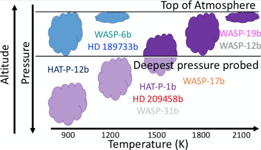
The curse of clouds 3

Figure 1. This schematic shows a typical hot Jupiter with an eastward-offset hot spot and superrotating winds, as observed during transit (left), eclipse (right) and
over a full phase curve (centre). The phase curve observation provides direct information about the spatial variability of the atmospheric temperature, whereas
the transit and eclipse observations average over the terminator and dayside respectively. This figure is reproduced from Barstow & Heng (2020) with permission
from Springer.

Figure 2. This figure illustrates the effect of clouds on the transmission spectrum of a planet. The black line in each panel shows how the transit depth varies
as a function of wavelength; larger transit depths correspond to starlight being absorbed at higher altitudes within the atmosphere. Different wavelengths are
indicated by multicoloured shading, and photons at particular wavelengths are shown as coloured arrows. The penetration altitude of each photon within the
atmosphere is shown by the vertical position of the arrow. The presence of clouds in the right hand panel can be seen to flatten and raise the lower part of the
spectrum, and prevents photons from reaching the deeper regions of the atmosphere.

 MNRAS 000, 1–9 (2021)

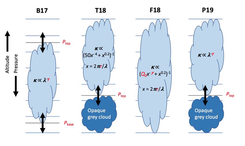
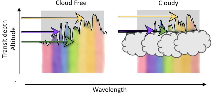
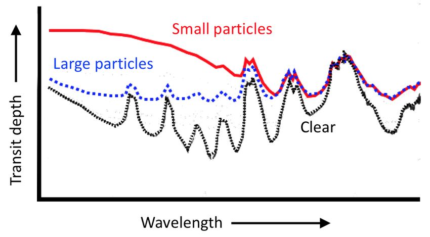
4 J. K. Barstow
 as well as additional data from the Spitzer space telescope; two
 others (Fisher & Heng 2018 and Tsiaras et al. 2018) considered only
 WFC3 spectra. All four papers adopt a minimal, parametric model
 to represent the effect of cloud and haze on the spectra, with each
 representation taking a slightly different approach to the problem.
 These different approaches are illustrated in Figure 4. Here, the
 opacity is a function of wavelength , and may also depend on
 effective particle radius ; a power law index ; and 0 , a factor
 that determines at what wavelength the scattering efficiency peaks.
 As well as the wavelength dependence of the opacity, a variety of
 different approaches are used to parameterise the height and vertical
 extent of the cloud. The model from Barstow et al. (2017), referred to
 as B17 in the diagram, has both variable cloud top and base pressures,
 whereas the Tsiaras et al. (2018) and Pinhas et al. (2019) (T18 and
Figure 3. The curves in this figure show transit spectra for a clear atmosphere
 P19) models have two distinct cloud regions, with the lower being a
(bottom), one with large cloud particles (middle) and small cloud particles
(top). Whilst both cloud types obscure gas absorption features, the large cloud
 completely opaque grey cloud deck, and the other having wavelength
particles introduce a flat bottom to the spectrum, whereas the small particles dependent opacity, with the pressure of the transition between them
create a slope with decreasing cloud opacity as a function of wavelength. being a free parameter. The Fisher & Heng (2018) model does not
 have an explicit parameterisation of vertical extent.
 In Barstow (2020), I conduct a comparative study of these differ-
chemistry atmospheric model with the choice of either an optimal ent methods for parameterising cloud in retrievals of transmission
estimation (Rodgers 2000) or the PyMultiNest (Buchner et al. 2014; spectra, by incorporating each of the models into NEMESIS and ap-
Feroz & Hobson 2008; Feroz et al. 2009, 2013) nested sampling plying them to the same two datasets; these are the STIS, WFC3 and
package, which is more commonly used for exoplanet applications Spitzer observations of hot Jupiters HD 189733b and HD 209458b.
(Krissansen-Totton et al. 2018). NEMESIS also uses the correlated- These planets are the two best-studied hot Jupiters, and have of-
k approximation (Lacis & Oinas 1991) to pretabulate the molecular ten been considered the archetypal ‘hazy’ and ‘cloudy’ hot Jupiters
absorption data, which rapidly reduces the computation time for the respectively.
forward model calculation.
 These characterisations were borne out by the analysis. Whilst the
 Because NEMESIS is free-chemistry, no physical constraints are
 different cloud models used fit for different variables, a consistent
placed on the abundances of the molecular and atomic species. It
 picture emerged for each planet when comparing the results. HD
is therefore possible to retrieve abundances that differ substantially
 189733b is best fit by a cloud with small effective particle radius
from the expected chemistry. Such results reveal either missing or
 /large power law index , and any grey cloud present is located deep
incorrect opacity within the NEMESIS model, or inadequacies in
 in the atmosphere, whereas the transparent, wavelength dependent
our physical understanding of the atmospheric system. Comparing
 portion of the cloud extends to low pressures. The converse is true
results from free retrievals with expectations from chemical models
 for HD 209458b, for which the opaque grey cloud dominates for the
provides us with useful insights that can further our understanding
 T18 and P19 models, and larger particle sizes/lower values of the
of atmospheric physics.
 power law index are favoured. This is consistent with expectations
 that small particles are more easily lofted high into an atmosphere
 and are therefore more likely to extend to lower pressures, whereas
3 REPRESENTING CLOUDS IN RETRIEVAL MODELS larger particles will sink and are more likely to be situated in the
 deeper regions.
The challenge for the inclusion of cloud or haze in retrieval models
is to represent it in a way that captures the important observable Whilst if cloud is not included at all in a retrieval model for a cloudy
impacts, whilst minimising the number of parameters used. The ap- planet the solution will be biased, reassuringly it seems that provided
proach taken will vary depending on the wavelength range covered the effects of the cloud are adequately represented the precise form
by the dataset and the geometry of the observation (transit or eclipse). of the representation doesn’t affect the retrieval of properties such
 In transit, the altitude of the cloud top has a particularly strong as the water vapour abundance. This is true at least for the datasets
effect on the spectrum (see Figure 2). The higher the cloud top, considered by Barstow (2020), although it may break down in the
the more it will obscure the molecular absorption features. There- context of higher precision spectra from JWST.
fore, some parameterisation of the vertical extent and position of the Parametric cloud models are clearly a powerful tool within exo-
cloud is critical to include. The wavelength dependence of the cloud planet retrieval. They are however somewhat divorced from physical
opacity will also be important; for particles that are small relative reality; for example, the power law index retrieved for HD 189733b
to the wavelength of light, the opacity will drop off rapidly as the takes values between 6 and 10. A purely Rayleigh scattering cloud
wavelength increases, whereas for larger particles the opacity will be would have an index of 4. Whilst for real clouds ’super Rayleigh’
relatively constant with wavelength (Figure 3). behaviour can occur over a narrow wavelength range (see Pinhas &
 The number density of cloud particles also has an impact on the Madhusudhan 2017), there is not an obvious mechanism to produce
spectrum, as this will influence the point at which the cloud becomes this over the full STIS—Spitzer range. Likewise, whilst the F18 pa-
opaque rather than transparent. rameterisation (based on the work of Kitzmann & Heng (2018) and
 Several studies have been published in recent years which attempt previously Lee et al. (2013)) does encode some indications of compo-
to characterise and compare a population of cloudy hot Jupiters sition via the 0 parameter, for the parameterised retrieval process
observed with HST. Two of these (Barstow et al. 2017 and Pinhas doesn’t make any physical assumptions about the availability of a
et al. 2019) considered data from the STIS and WFC3 instruments, suitable condensate. Therefore, gaining detailed understanding of

MNRAS 000, 1–9 (2021)

The curse of clouds 5

Figure 4. This figure shows the different simple cloud parameterisations that have been used in recent comparative studies of transiting exoplanets. It illustrates
how various free parameters, including cloud top and base pressures ( base and top ), effective particle radius ( ), scattering index ( ) and peak extinction factor
( 0 ) are used to describe the cloud in the four studies (Barstow et al. 2017; Tsiaras et al. 2018; Fisher & Heng 2018; Pinhas et al. 2019).

the physical properties of cloud requires more than just a parametric will condense. In reality, saturation above the saturation vapour pres-
model framework. sure is often required for condensation to take place as the curvature
 of a liquid droplet represents an additional energy barrier to conden-
 sation due to increased surface tension for small particles. However,
 this is to first order a reasonable approximation.
4 PHYSICAL CLOUD MODELS
 The vertical extent of the cloud deck and the size of the cloud
Parametric retrieval models are at the simple end of a continuum of particles above the base of the cloud are determined by the balance
cloud models with varying complexity. The degree to which a model of upward vertical mixing via eddy diffusion, and downward sedi-
contains detailed physics is generally a trade off against computation mentation of the particles. The motion of the particles is described
time and flexibility. It is not feasible, as yet, to couple fully con- by the equation
sistent microphysical cloud models to an inversion algorithm, since
retrievals using Markov-Chain Monte Carlo or nested sampling tech-
 
niques generally require several tens of thousands of individual model − rain ∗ = 0 (3)
calculations as a minimum, so a single forward model run must be 
rapid. where is the eddy diffusion coefficient, ∗ is the convective
 velocity scale rain is the sedimentation efficiency, is the altitude,
 and and are the total and condensate mole fractions of the
4.1 The Ackerman and Marley model condensing species. The distribution of particle sizes in the model is
Approaches such as that of Ackerman & Marley (2001) provide a represented by a log-normal distribution. The geometric mean radius
 1/ 
good compromise. This model incorporates a simplified represen- of the distribution scales with . The power law index takes
tation of condensation and sedimentation/rainout of cloud particles, values between 1 and 2 can be defined by fitting the particle fall
which can be described with only a few variables. Models of this speeds for different radii around the point where the velocity is equal
type can be used in conjunction with retrieval algorithms as the com- to the convective velocity scale ∗ ; in practice, it is often held fixed
putation time is still relatively rapid; at the expense of having to to an intermediate value such as 1.4 (Charnay et al. 2018).
make some assumptions, the results from a retrieval analysis can be A cloud deck that is self-consistent with the temperature profile
directly related to physical processes within the atmosphere. and condensate abundance can thus be calculated using this method
 The Ackerman and Marley (hereafter AM01) model works by as- with as few as two extra free parameters, and . A typical
suming that all excess vapour beyond the saturation vapour pressure cloud deck generated using the AM01 model is shown in Figure 5.

 MNRAS 000, 1–9 (2021)

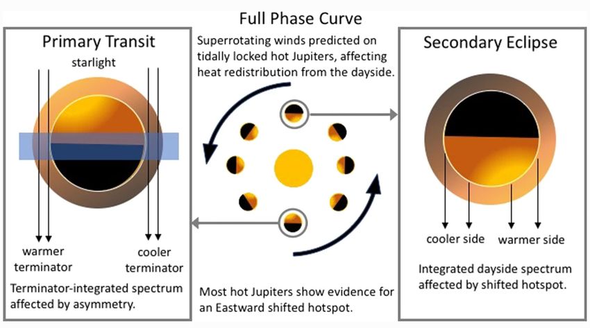
6 J. K. Barstow
This does however require some further underlying assumptions. Temperature (K)
For example, the saturation vapour pressures of likely condensates 1000 1200 1400 1600 1800 2000
 10 4
must be calculated and included, and likely condensates must also cloud
be included in the model atmosphere in vapour form. In some cases, total
 10 3
 SVP
the condensate vapour might have spectral features within the wave-
length range studied, but this will not be universally true; therefore

 Pressure (bar)
 10 2
independent constraint on the amount of vapour available for con-
densation may not be possible. Nonetheless, the model represents a
good compromise between minimal free parameters, relatively rapid 10 1

computation time, and a basis in atmospheric physics.
 Mai & Line (2019) explore the application of different param- 100
eterised cloud models to simulated JWST datasets. They generate
the datasets using the AM01 cloud model, and explore the extent 101
 10 8 10 7 10 6 10 5 10 4
to which simpler, less physical parameterisations can recover the Mixing ratio
key characteristics of the cloud. They find that the atmospheric gas
phase composition is relatively robust to different cloud models, as
in Barstow (2020), but unsurprisingly that the recovery of cloud Figure 5. This plot shows the structure of a cloud generated using the AM01
properties is very dependent on the choice of cloud model. They model prescription. The temperature-pressure profile is shown in yellow, and
recommend that the AM01 cloud model is used in all cases where the total mixing ratio of the condensate is shown in red. The black dashed
the goal is to obtain information about the cloud itself. line is the saturation vapour pressure. The cloud starts to form where the
 condensate mixing ratio crosses the saturation vapour pressure curve. The
 mixing ratio of the condensed cloud is shown in blue. The mixing ratio of the
4.2 Microphysical and kinetic simulations condensate is constant below the cloud, but decreases with decreasing pres-
 sure above the base of the cloud due to sedimentation of the cloud particles.
It is also possible to simulate the microphysical processes of cloud
 This figure is reused from Yang (2020) with the permission of author.
formation, and generate synthetic spectra based on these models.
The computation time prohibits these models from being coupled to
a retrieval algorithm; however, as a purely forward modelling tool that the retrieved characteristics of cloud can be explained by two
these simulations can be very informative. Gao et al. (2020) apply the different types of cloud, which condense at different temperatures. As
Community Aerosol Radiation Model for Atmospheres (CARMA) planet temperature increases, a given cloud will be forced to form at
to hot Jupiter atmospheres, to investigate haze and cloud formation higher regions in the atmosphere where it is cooler, until it is unable
over a range of temperatures. CARMA explicitly models the nu- to condense at all. In Gao et al. (2020), the species responsible for
cleation of cloud particles, both homogeneous (self-nucleation) and this sort of pattern are identified as hydrocarbon haze and silicates.
heterogeneous (nucleating onto a particle of another substance); con- Larger cloud particles are expected to reside deeper in the at-
densational growth and evaporation; and coagulation. It also deals mosphere, and indeed in B17 we found that the deepest visible
with the vertical transport of the particles that are formed. This pro- clouds were found on planets with temperatures around 1500 K.
cess allows the cloud formation to be modelled from first principles, This corresponds to the temperature at which the cloud particle size
and does not require assumptions to be made about parameters that is maximised in the Gao et al. (2020) study. This agreement between
do not have a direct physical meaning. observation-driven and detailed modelling studies is very encour-
 Whilst microphysics models are too complex and time consuming aging; it indicates that our understanding of the physics of cloud
to be used in a retrieval context, their results can still be compared formation in hot atmospheres is reasonably correct. It also highlights
with available datasets. Gao et al. (2020) examine the formation of the importance of applying models of various levels of complexity
cloud and haze on planets at different temperatures, and compare the to the problem.
results to the observed amplitude of the H2 O absorption feature in Other groups have also made use of this type of modelling. A con-
the Hubble/WFC3 bandpass. The amplitude of this feature is affected siderable body of work on dust grain formation in brown dwarf and
by the presence of cloud and haze, as explained in Section 1.3. For stellar atmospheres is encapsulated in the development of the DRIFT
very cloudy atmospheres, the feature can be almost non-existent, so code (Woitke & Helling 2003, 2004; Helling & Woitke 2006; Helling
the planets with the lowest amplitude water features are likely to be et al. 2008). This code considers the formation of condensation nu-
cloudy. By contrast, planets with semi-transparent high altitude haze clei that might facilitate the formation of clouds in hot atmospheres,
might still have substantial water vapour absorption features, depend- as well as the formation of dust and clouds themselves. Elements
ing on the size of the haze particles; if the particles are small, the of the DRIFT code have also been incorporated into global climate
extinction efficiency may be relatively small in the WFC3 bandpass. models, which allows the 3D effects of cloud to be investigated.
 Gao et al. (2020) find that the spectra of hot Jupiters with tem-
peratures ranging from less than 1000 K to over 2000 K are mostly
dominated by silicate clouds, with hydrocarbon hazes playing a part
 4.3 Cloud in Global Climate Models
for only the coolest planets. They find that cloud coverage varies
considerably as a function of temperature, with the smallest H2 O ab- In recent years, clouds have begun to be incorporated into Global
sorption features in the modelled spectra occurring at temperatures Climate Models (GCMS). In some cases, this has been simply as a
around 1700 K. This matches the feature amplitudes from observa- passive tracer, whilst in others the radiative feedback effects of the
tional data remarkably well. The largest cloud particles are formed cloud have also been included.
at temperatures of around 1500 K. Parmentier et al. (2016) use the results from an existing 3D GCM
 The results from the Gao et al. (2020) model echo the findings of to predict where various clouds will form in an exoplanet atmosphere.
Barstow et al. (2017). In Figure 6, taken from the B17 paper, we see Clouds form where the partial pressure of the condensate exceeds the

MNRAS 000, 1–9 (2021)

The curse of clouds 7

Figure 6. This figure from Barstow et al. (2017) presents a hypothesis that can explain the retrieved cloud top pressures, and the preference for Rayleigh vs grey
wavelength dependence, from the study. The two different colours represent two different condensibles that form cloud at different temperatures. As planets
become hotter, any particular cloud will form higher up in the atmosphere assuming the temperature decreases with altitude. At high enough temperatures, some
clouds will be unable to condense, and their place will be taken by cloud species with a higher vaporisation temperature.

saturation vapour pressure for that species. The cloud particle size, for a variety of modelling scenarios that can then be compared with
and the location of the cloud top, are both free parameters within the observations.
model; sedimentation and growth processes are not considered. Simulated observations can also be used to generate datasets for
 planets as they would be seen for future instruments. As the commu-
 This equilibrium cloud condensation model indicates that different
 nity prepares for the launch of JWST, and with increasing awareness
types of cloud that form at different temperatures would affect the
 that the 3D structure of exoplanet atmospheres is likely to signifi-
shape of an optical phase curve of the planet, with the peak occurring
 cantly influence what we see, the development of tools such as this
at different phases depending on what type of cloud has formed. This
 is especially timely.
is due to the large temperature variation as a function of phase,
which means that cloud forms in some locations but not in others.
Parmentier et al. (2016) suggest that the location of the optical phase
curve maximum can be used as a diagnostic for particular cloud
 5 EXOPLANET CLOUDS IN THE JWST ERA
species.
 Given the expectation that JWST will be a game changer for the ob-
 Lee et al. (2016) incorporate the DRIFT kinetic cloud model into
 servation of exoplanet atmospheres, a substantial amount of effort
a 3D radiative hydrodynamic simulation of the atmosphere of hot
 has been invested in simulating JWST spectra. This enables the com-
Jupiter HD 189733b. In this case, the cloud is fully coupled to the
 munity to make informed decisions about which targets to observe,
dynamics and radiative transfer; the cloud formation is governed by
 and to test the tools we plan to use for interpretation.
the local thermal conditions, and in turn the radiative properties of
 Some early efforts to simulate JWST spectra, by Barstow et al.
the cloud feed back into the temperature structure. The simulation
 (2015) and Greene et al. (2016), used simple 1D parameterised at-
reveals a cloud concentrated in the nightside equatorial regions of the
 mospheric retrieval models to test what sort of information could
planet. The deeper regions of the cloud are dominated by magnesium
 be recovered from observations. These did not include complex or
silicate, but at higher altitudes uncovered seed particles of titanium
 sophisticated cloud models; Barstow et al. (2015) considered mostly
dioxide are present.
 cloud-free atmospheres, with the exception of a single simulation
 Lines et al. (2018) build on the work of Lee et al. (2016) and for GJ 1214b, and Greene et al. (2016) included examples with only
incorporate key elements of the DRIFT code into the Unified Model, a simple opaque grey cloud deck, which was assumed to cover the
which has been expanded in recent years to simulate hot Jupiter planet.
spectra. This model incorporates cloud formation and radiative feed- Wakeford & Sing (2015) produce synthetic JWST spectra for a
back, and the authors also generate simulated transmission spectra range of species. Whilst they do not perform a retrieval test to exam-

 MNRAS 000, 1–9 (2021)

8 J. K. Barstow
ine the recoverability of information, the simulations reveal that ab- & Burrows (2020b) find that in many cases the composition of the
sorption features for multiple cloud species occur towards the longer aerosol can be distinguished from JWST spectra, although this is
end of the JWST wavelength range. Therefore, with JWST direct more challenging in the case of different hydrocarbon hazes as their
detection of particular cloud constituents would be possible. spectra closely resemble each other.
 Due to the required speed of computation for retrieval models that
rely on either MCMC or Nested Sampling for iterating towards a
preferred solution, multiple scattering in clouds has generally been
ignored for exoplanets. Whilst several examples exist of multiple 6 CONCLUSIONS
scattering clouds being modelled in the Solar System, these simula- The launch of JWST is expected to provide considerable insights into
tions are usually coupled to an algorithm such as Optimal Estimation cloudy exoplanets. For example, we hope for the first time to obtain
(Rodgers 2000), which requires only a few tens of forward modelling observational evidence for the composition of the clouds present in
runs to arrive at a solution. Barstow et al. (2014) did model multi- hot Jupiter atmospheres, which the JWST wavelength coverage will
ple scattering in order to characterise the reflected starlight from hot allow. Characterising cloud more fully across a range of planets with
Jupiter HD 189733b, but only in the context of forward modelling different atmospheric conditions will provide additional information
rather than retrieval. about dynamics and thermal structure, since cloud formation is in-
 Indeed, the majority of exoplanet retrieval models adopt an trinsically tied to atmospheric circulation and convection.
extinction-only approximation. This results in all photons that in- A range of modelling approaches will be required to fully ex-
teract with a cloud particle being either absorbed or scattered out ploit these datasets. Interpretation of observations will require re-
of the beam. In reality, depending on the single scattering albedo trievals and parameterised models, which will necessarily be more
(the fraction of light scattered vs absorbed) and the scattering phase sophisticated than those that are currently available. The recent work
function (which direction photons are preferentially scattered in), highlighted here has provided several possible avenues for this de-
some percentage of photons that interact may be forward-scattered velopment, with the following factors being key considerations:
and remain within the beam, and some that are scattered out may be
scattered back into the beam due to interaction with another particle. • Spatial variation in cloud coverage
Full treatment of scattering in models can, therefore, result in very • Spatial variation in temperature
different results to the extinction-only approximation, depending on • Inclusion of scattering in eclipse spectra
the characteristics of the cloud. 3D climate simulations that contain physically motivated cloud
 Taylor et al. (2020) investigate the impact of including scattering models will be an important resource for benchmarking new mod-
on eclipse spectra of hot Jupiters as seen with JWST. Whilst they do els and methods (e.g. Barstow et al. 2019). Testing the ability of a
not perform a full multiple scattering calculation, they do consider retrieval to correctly recover a known solution is an important vali-
scattering as distinct from extinction. The major impact of this is that dation step, and physical simulations inform us about the phenomena
the atmosphere no longer emits as a blackbody. This can lead, for we should be able to recover.
example, to emission features appearing in a spectrum even in the Community level efforts have ensured open access to Cycle 1 data
case where the atmosphere is isothermal. from JWST via the Early Release Science programme, and similar
 Taylor et al. (2020) use their scattering model to investigate the strategies are now underway to discuss and implement necessary
biases that would result from fitting a spectrum of a planet with scat- developments in modelling tools - for example, the January 2021
tering cloud with a model assuming pure absorption. They find that Specialist Discussion Meeting on Exoplanet Modelling in the JWST
atmospheric temperatures would be consistently underestimated in Era. The next few years will no doubt be an exciting time, with a
this case. They also develop a simple parameterised model that is able fair share of new (and perhaps controversial!) discoveries; my hope
to account for different degrees of scattering, by fitting for the single is that the community will build on the current collaborative spirit as
scattering albedo. The single scattering albedo is parameterised as a we further our understanding of these fascinating worlds.
step function, with a shift between two variable values at a variable
wavelength. This is quite representative of the wavelength-dependent
single scattering albedo for a typical cloud.
 As well as the need to consider scattering, spatial variation of ACKNOWLEDGEMENTS
cloud coverage and temperature is also a key concern for interpreting I thank Jingxuan Yang, who recently worked with me as a Masters
JWST data. Line & Parmentier (2016) consider the effect of any cloud student, for his excellent work implementing the AM01 model in
present covering only a fraction of the terminator region. Subsequent NEMESIS, and for giving me permission to use an explanatory figure
authors have built on this to consider the effect of atmospheric spatial from his thesis. For the majority of my own work that I discuss in the
variability on observed spectra. Recently, Lacy & Burrows (2020a) article I was supported by the Royal Astronomical Society Research
examined the effect of strong temperature gradients in the presence Fellowship. I am currently an Ernest Rutherford Fellow supported by
of cloud and haze on exoplanet transmission spectra. They find that the Science and Technology Facilities Council.
cloud and haze exacerbates the impact on observed spectra of strong
day-night temperature gradients, making it even more critical to ac-
count for this.
 In Lacy & Burrows (2020b) they further investigate the possibility REFERENCES
of recovering information about cloud from JWST spectra, using
 Ackerman A. S., Marley M. S., 2001, ApJ, 556, 872
relatively simple cloud models where the cloud is treated either as 1) Arcangeli J., et al., 2019, A&A, 625, A136
a well mixed slab up to a certain top pressure, or 2) an equilibrium Barstow J. K., 2020, MNRAS, 497, 4183
cloud that condenses once saturation is reached, with a number of Barstow J. K., Heng K., 2020, Space Sci. Rev., 216, 82
particles that drops off towards lower pressures according to a power Barstow J. K., Aigrain S., Irwin P. G. J., Hackler T., Fletcher L. N., Lee J. M.,
law with a variable index. Regardless of the model adopted, Lacy Gibson N. P., 2014, ApJ, 786, 154

MNRAS 000, 1–9 (2021)

The curse of clouds 9
Barstow J. K., Aigrain S., Irwin P. G. J., Kendrew S., Fletcher L. N., 2015, Waldmann I. P., 2016, ApJ, 820, 107
 MNRAS, 448, 2546 Woitke P., Helling C., 2003, A&A, 399, 297
Barstow J. K., Aigrain S., Irwin P. G. J., Sing D. K., 2017, ApJ, 834, 50 Woitke P., Helling C., 2004, A&A, 414, 335
Barstow J., Lines S., Mayne N., Manners J., Boutle I., Lee G., Irwin P., Helling Yang J., 2020, Master’s thesis, University College London
 C., 2019, in EPSC-DPS Joint Meeting 2019. pp EPSC–DPS2019–1505 Zhang M., Chachan Y., Kempton E. M. R., Knutson H. A., 2019, PASP, 131,
Benneke B., 2015, arXiv e-prints, p. arXiv:1504.07655 034501
Buchner J., et al., 2014, A&A, 564, A125
Caldas A., Leconte J., Selsis F., Waldmann I. P., Bordé P., Rocchetto M., This paper has been typeset from a TEX/LATEX file prepared by the author.
 Charnay B., 2019, A&A, 623, A161
Charbonneau D., Brown T. M., Noyes R. W., Gilliland R. L., 2002, ApJ, 568,
 377
Charnay B., Bézard B., Baudino J. L., Bonnefoy M., Boccaletti A., Galicher
 R., 2018, ApJ, 854, 172
Evans T. M., et al., 2013, ApJ, 772, L16
Feroz F., Hobson M. P., 2008, MNRAS, 384, 449
Feroz F., Hobson M. P., Bridges M., 2009, MNRAS, 398, 1601
Feroz F., Hobson M. P., Cameron E., Pettitt A. N., 2013, preprint,
 (arXiv:1306.2144)
Fisher C., Heng K., 2018, MNRAS, 481, 4698
Gandhi S., Madhusudhan N., 2018, MNRAS, 474, 271
Gao P., et al., 2020, Nature Astronomy, 4, 951
Greene T. P., Line M. R., Montero C., Fortney J. J., Lustig-Yaeger J., Luther
 K., 2016, ApJ, 817, 17
Helling C., Woitke P., 2006, A&A, 455, 325
Helling C., Dehn M., Woitke P., Hauschildt P. H., 2008, ApJ, 675, L105
Irwin P. G. J., et al., 2008, JQSRT, 109, 1136
Kitzmann D., Heng K., 2018, MNRAS, 475, 94
Kreidberg L., et al., 2014, Nature, 505, 69
Kreidberg L., et al., 2018, AJ, 156, 17
Krissansen-Totton J., Garland R., Irwin P., Catling D. C., 2018, AJ, 156, 114
Lacis A. A., Oinas V., 1991, J. Geophys. Res., 96, 9027
Lacy B. I., Burrows A. S., 2020a, arXiv e-prints, p. arXiv:2006.06899
Lacy B., Burrows A., 2020b, arXiv e-prints, p. arXiv:2007.00109
Lavie B., et al., 2017, AJ, 154, 91
Lee J.-M., Heng K., Irwin P. G. J., 2013, ApJ, 778, 97
Lee G., Dobbs-Dixon I., Helling C., Bognar K., Woitke P., 2016, A&A, 594,
 A48
Line M. R., Parmentier V., 2016, ApJ, 820, 78
Line M. R., Knutson H., Wolf A. S., Yung Y. L., 2014, ApJ, 783, 70
Lines S., et al., 2018, MNRAS, 481, 194
MacDonald R. J., Madhusudhan N., 2017, MNRAS, 469, 1979
MacDonald R. J., Goyal J. M., Lewis N. K., 2020, ApJ, 893, L43
Mai C., Line M. R., 2019, ApJ, 883, 144
Min M., Ormel C. W., Chubb K., Helling C., Kawashima Y., 2020, A&A,
 642, A28
Mollière P., et al., 2020, A&A, 640, A131
Nikolov N., et al., 2018, Nature, 557, 526
Parmentier V., Fortney J. J., Showman A. P., Morley C., Marley M. S., 2016,
 ApJ, 828, 22
Pinhas A., Madhusudhan N., 2017, MNRAS, 471, 4355
Pinhas A., Rackham B. V., Madhusudhan N., Apai D., 2018, MNRAS, 480,
 5314
Pinhas A., Madhusudhan N., Gandhi S., MacDonald R., 2019, MNRAS, 482,
 1485
Rodgers C. D., 2000, Inverse Methods for Atmospheric Sounding. World
 Scientific
Stevenson K. B., et al., 2014a, Science, 346, 838
Stevenson K. B., Bean J. L., Madhusudhan N., Harrington J., 2014b, ApJ,
 791, 36
Taylor J., Parmentier V., Line M. R., Lee G. K. H., Irwin P. G. J., Aigrain S.,
 2020, arXiv e-prints, p. arXiv:2009.12411
Tsiaras A., et al., 2018, AJ, 155, 156
Vidal-Madjar A., et al., 2011, A&A, 527, A110
Wakeford H. R., Sing D. K., 2015, A&A, 573, A122
Wakeford H. R., et al., 2017a, Science, 356, 628
Wakeford H. R., Visscher C., Lewis N. K., Kataria T., Marley M. S., Fortney
 J. J., Mand ell A. M., 2017b, MNRAS, 464, 4247
Wakeford H. R., et al., 2018, AJ, 155, 29

 MNRAS 000, 1–9 (2021)