Raptor Feeding Characterization and Dynamic System Simulation Applied to Airport Falconry - MDPI
←
→
Page content transcription
If your browser does not render page correctly, please read the page content below
sustainability

Article
Raptor Feeding Characterization and Dynamic
System Simulation Applied to Airport Falconry
José Luis Roca-González 1, * , Antonio Juan Briones Peñalver 2
and Francisco Campuzano-Bolarín 2
 1    Department of Engineering and Applied Technologies,
      University Centre of Defence at the Spanish Air Force Academy, 30720 Santiago de la Ribera, Spain
 2    Department of Business Economics, Universidad Politécnica de Cartagena, 30201 Cartagena, Spain;
      aj.briones@upct.es (A.J.B.P.); Francisco.campuzano@upct.es (F.C.-B.)
 *    Correspondence: jluis.roca@cud.upct.es

 Received: 25 September 2020; Accepted: 17 October 2020; Published: 27 October 2020

 Abstract: Airport falconry is a highly effective technique for reducing wildlife strikes on aircraft,
 which cause great economic losses. As an example, nowadays, wildlife strikes on aircrafts in the air
 transport industry are estimated to cost between USD 187 and 937 million in the US and USD 1.2 billion
 worldwide every year. Moreover, the life-threatening danger that wildlife strikes pose to passengers
 has prompted security stakeholders to develop countermeasures to prevent wildlife impacts near
 airport transit zones. The experience acquired from international countermeasure analysis reveals
 that falconry is the most effective technique to create sustainable wildlife exclusion areas. However, its
 application in airport environments continues to be regarded as an art rather than a technique;
 falconers modulate raptors’ behavior by using a trial-and-error system of controlling their hunger to
 stimulate the need for prey. This paper focuses on a case study where such a decision-making process
 was designed as a dynamic system applied to feeding planning for raptors that can be used to set
 an efficient baseline to optimize raptor responses without damaging existing wildlife. The results
 were validated by comparing the outputs of the model and the falconer’s trial-and-error system,
 which revealed that the proposed model was 58.15% more precise.

 Keywords: wildlife exclusion areas; airport falconry; raptor behavior; dynamic system simulation

1. Introduction
     The expenses incurred by the US civil air transport industry resulting from wildlife strikes, which
cost between USD 187 and 937 million annually over a period of 24 years [1], agree with the figures in
international studies. These investigations estimated that the average cost of an occurrence of this
type is approximately USD 200,000 [2–4], excluding the effects of fatal accidents, where the cost of
lost human life goes beyond the economic impact. Therefore, because wildlife near airports and air
transit areas increase the risk of such an event, it is considered a real and serious threat to passengers,
aircraft crew, and the air transport industry in general [5]. These circumstances prompted airport
managers and security stakeholders [6] to develop procedures to prevent wildlife hazards in airport
landscapes. Exclusion areas for wildlife in airport transit zones were created by deploying as many
countermeasures as possible.
     The results derived from international case studies [7–12] revealed that falconry is the most
effective technique to create exclusion areas. However, a deeper analysis of the present falconry
methods should be critiqued. Falconry has to be defined as a combination of science and art, rather
than merely an art [13,14], as it is usually practiced. Typically, a falconer develops a feeding process for
each raptor based on personal experience that simply forces the raptor to hunt when it is released.

Sustainability 2020, 12, 8920; doi:10.3390/su12218920                       www.mdpi.com/journal/sustainability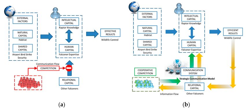
Sustainability 2020, 12, 8920                                                                        2 of 21

      Airport falconry has been estimated to cost approximately USD 130,000 for 24 h of service
and USD 65,000 for 8 h of service at airports of any size [2]; meanwhile, others have estimated
USD 25,000–150,000 [1] or 30,000–50,000 for medium-sized airports [15] for low-operation seasons,
nearly USD 950–2900 per week during peak seasons [16] or USD 50,000 per year in other cases [17],
and nearly USD 337,500 [18] for bigger airports. Airport safety managers therefore focus on increasing
the efficiency of airport falconry [19] to reduce expenses, but also on preserving its performance
and capability to create exclusion areas within the airport limits.
      Currently, falconry is characterized by a trial-and-error process where falconers identify
the “right-hunger” point of each raptor through a self-learning process that finally becomes part of
their expertise, which is typically concealed from potential competitors. Consequently, falconry has
become an ineffective process that lacks broad ornithological knowledge. Accordingly, falconers need
to improve their own learning curve as opposed to having a conceptualization of standard techniques.
Advantages could be acquired from other experiences in order to set standards that could enable
replication when employed in case studies. This type of knowledge, developed by each falconer, is
part of the intellectual capital that has accumulated and derived from the experiences of generations of
falconers or records that they may have kept regarding trial-and-error feeding routines that encourage
raptors to hunt for prey when they are released. The specific feeding timetables that lead raptors to
obtain the best and safest hunting results when released, based on what is known as the right-hunger
point, are crucial for understanding the feeding decision process that airport falconers should follow.
      The goal of this research was to analyze a case study in which an airport falconer’s knowledge is
systematically and thoroughly examined in order to model a dynamic system design that could help
falconers to perform their job more efficiently. This is made possible by baseline results that can be used
to predict the raptor status, which can aid in the decision-making process related to the modulation of
raptor feeding to encourage the raptors to maintain the right hunting actions as an example of applying
simulations to a practical case study [20].
      To achieve this goal, it was necessary to first develop a methodological analysis of a case study
based on experiences obtained from the Civil and Military Airport of San Javier (IATA: MJV, OACI:
LELC), which is located in the southeast of Spain at latitude 37.7785 and longitude −0.808289. This
airport has two operating runaways: 05 R/23 L, which is 2.300 m long and is used for military purposes
only (CASA C-101 and E-26 Tamiz), and 05 L/23 R, which is 1.580 m long and was previously used for
civil purposes (Boeing 757 or Airbus A321) until January 2019, when the new International Airport
of Murcia was put into service; since then, MJV has been reserved for military use only. Civil transit
statistics show that the median value of air operations was 9081 flights in 2018 and nearly 1,095,471
passengers in 2017. Since 2019, the statistical information regarding aircraft operations has not been in
the public domain due to its military implications.
      Regarding the airport wildlife control service, its assistance made it possible for us to access
the daily feeding records of raptors that the airport employed over 10 years (2004–2014). The statistical
analysis summarizing several allometric equations that linked the feeding of raptors with the best
results when they were released was also accessed. That previous research made it possible to advance
to a second stage, where simulation software was utilized to create a dynamic system model that can
support future decision-making processes related to airport falconry.
      This paper has several sections that explain the following: the typical organization of
wildlife control services at airports, the systemic approach analogy, the dynamic model proposal,
and the simulations performed with Vensim software to create feeding tables.

2. Materials and Methods

2.1. Wildlife Control Services and Airport Falconry
    The wildlife control service (WCS) employed in airport environments is complex (Figure 1),
involving the relational capital of falconers combined with facilities, infrastructures, techniques,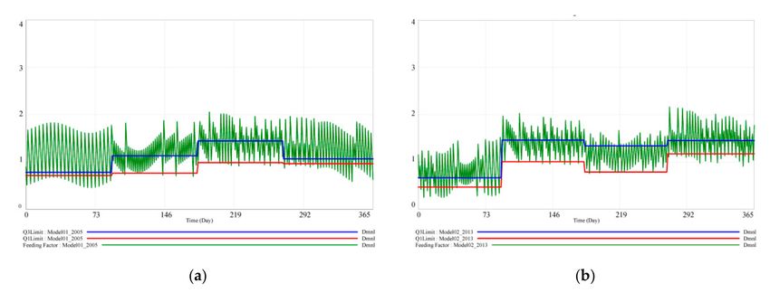
Sustainability 2020, 12, 8920                                                                                 3 of 21

knowledge, and added value resources in order to create wildlife exclusion areas [21]. Airport
falconry, following the instructions of the airport services manual from the International Civil Aviation
Organization [22], is an essential part of the task that the WCS performs in combination with other
techniques. Airport falconry is considered one of the most effective techniques implemented by
the WCS [7]. However, it should be considered as a variation of common falconry techniques in which
raptors are typically used to hunt injured or dead prey without intervention. Moreover, airport falconry
must preserve wildlife within the bounds of the airport [23]. This prompts falconers to develop tedious
training systems for raptors to make them return when a decoy is shown, including the use of tricks
that warn the wildlife of the raptor’s presence in the exclusion area, such as small bells or warning
systems using sound.

      Figure 1. Airport wildlife control service: knowledge management study of airport falconry. Source: [14].

      As described above, the aim of airport falconry is to create wildlife exclusion areas rather than to
kill prey. Therefore, to understand its implications, it should be redefined as the daily release of trained
raptors in airport fields to warn the wildlife in the area of the raptor hunting zones; consequently, this
will condition the wildlife to stay away from these zones. Moreover, airport falconry uses modifications
of traditional falconry in order to prevent mortality during this activity, thus allowing the coexistence
of wildlife and air transport operations.

2.2. Knowledge and Infrastructure Characterization
     WCS knowledge is characterized by intellectual capital and relational knowledge. Intellectual
capital refers to the skill in the use of raptors in two aspects: internal and external. Examples of
internal factors include the raptor training program, the release technique, and the feeding process.
The external aspects depend on the information gained from each airport, such as knowledge of
ornithology and habitats, transit operation ratio, airport design, maintenance weaknesses that offer
hiding places for wildlife, and even any possible blockage of water in drainage grates that attract
wildlife, among other factors.
     The WCS facilities are characterized by the housing provided for birds of prey. This includes all
equipment and workspace needed for falconers to care for and feed the raptors. The housing should
have enclosed and open areas that can support these activities (Figure 2). Furthermore, the housing
must have artificial places that resemble the raptors’ natural environment to reduce their stress.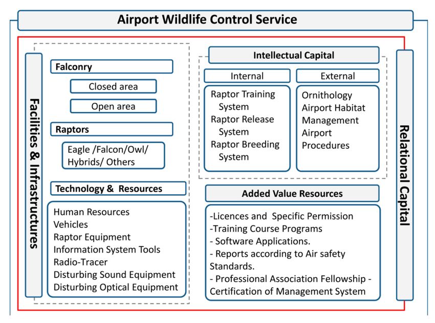
Sustainability 2020, 12, 8920                                                                         4 of 21

According to some examples and expert recommendations, the total of both areas should provide
a surface area of 3.5 m2 per raptor.
     Raptors are defined as a group of birds that have common relatives with genetic and anatomic
similarities, such as strong claws, sharp nails, and curved and hooked beaks; these birds usually
capture prey with their claws [24]. Raptors can be divided into five taxonomic groups: Cathartidae,
Pandionidae, Accipitridae, Sagittarius, and Falconidae for diurnal raptors, and Strigiformes (Strigidae
and Tytonidae) for nocturnal raptors [25].

                        Figure 2. Airport falconry infrastructure: housing for birds of prey [26].

      Airport activity has encouraged falconers to simplify the classification into two main groups
according to the raptor’s hunting strategy (Table 1). Thus, most airport services require some raptors
for high-altitude flights and other raptors for low-altitude or hand-to-hand flights. According to this
classification, raptors for the high-altitude range take advantage of the potential energy they gain
as they fall at a high speed over their prey; this allows them to hunt bigger prey while consuming
less energy. Meanwhile, this can increase the potential prey’s awareness of the raptors’ presence
and encourage them to recognize the exclusion area limits. On the other hand, for the low-altitude or
hand-to-hand range, raptors use short and fast flights that are considerably closer to the ground than
the flights of raptors at a high altitude. Consequently, this disperses the wildlife from covered zones
inside the exclusion area.
      As there is a clear difference in the hunting strategy between these two types of raptor, it is
evident that the energy consumption required for hunting should also be different. In order to apply
a systemic approach, the raptors were considered as a “black box”, where the main input is feeding
and the output is weight plus an evaluation of the hunting flight when the raptor is released. Therefore,
the type of raptor for this research did not affect the systemic characterization of the process by defining
the specific parameters for each raptor and the generic model. Thereafter, this would allow the analysis
of the reliability and accuracy of each model.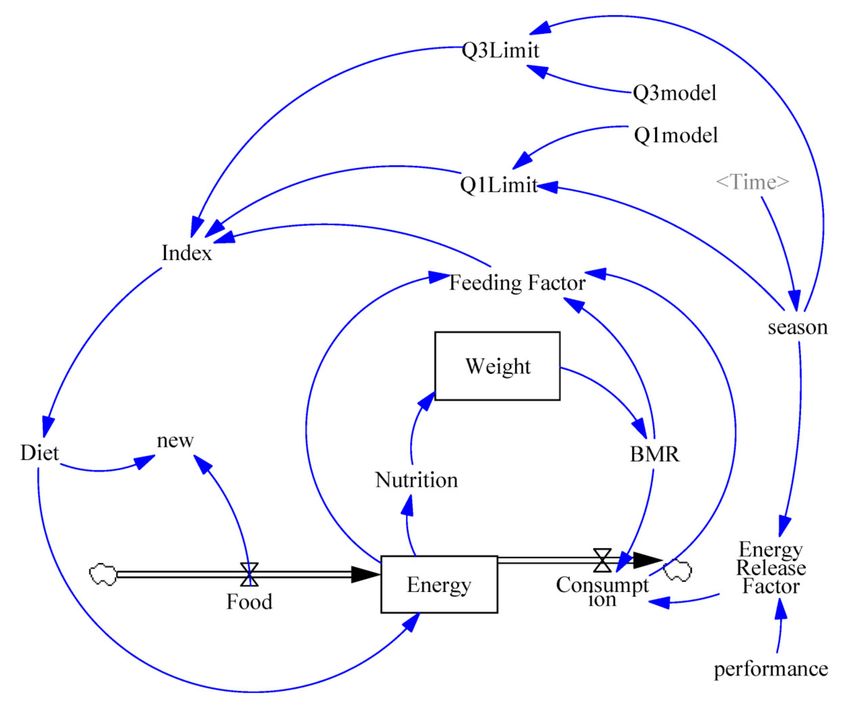
Sustainability 2020, 12, 8920                                                                                          5 of 21

                                Table 1. Typical raptors used by wildlife control service (WCS).

                            Height         Wingspan        Weight
  Raptor         Sex                                                                   Main Characteristics
                             (cm)            (cm)           (g)
                                               Low-altitude or hand-to-hand flights
 Accipiter        M             49–56        93–105        510–1170      Strong, nervous, with delicate feathers; males are
 Gentilis         F             58–64       108–127        820–1500     better for feathered prey and females for hairy prey
 Accipiter        M             29–34         58–65         110–200           Nervous, aggressive, fast metabolic rate
  Nisus           F             35–41         67–80         185–340            Appropriate for preying on other birds
 Parabuteo        M             50–60       103–125         450–750                   Calm, slow metabolic rate
 Unicinctus       F             50–60       103–125        750–1200         Ideal for preying on rabbits, hares, squirrels
   Buteo          M             45–56       105–135        690–1300                   Calm, low metabolic rate
 Jamaicensis      F             50–65       105–135        900–1460         Ideal for on preying rabbits, hares, squirrels
   Bubo           M             60–75       160–188       1580–3000                        Calm and tough
   Bubo           F             60–75       160–188       1750–4000                 Appropriate for night hunting
  Aquila          M              ~80          ~200        2650–3800             Aggressive, with slow metabolic rate
 Chrysaëtos       F              ~80          ~200        3600–4600          Requires a big area for flying and hunting
                                                      High-altitude flights
   Falco          M             38–45        89–100       600–700                    Calm, medium resistance
  Peregrinus      F             46–51       104–113      850–1300                Perfect for hunting feathered prey
   Falco          M              ~53        110–120      850–1200       Strong, good behavior when released hand-to-hand
  Rusticolus      F              ~56        120–130     1300–2100             Appropriate for hunting feathered prey
   Falco          M              ~45        100–110       730–990               High resistance, slow metabolic rate
  Cherrug         F              ~55        120–130      970–1300                   Perfect for any kind of prey
   Falco          M             35–40        90–100       500–600
                                                                             Considerably quiet, with high resistance
  Biarmicus       F             45–50       100–110       700–900
   Falco          M             25–30         50–62       125–250                  Nervous, high metabolic rate
  Columb.         F             25–30         50–62       150–300                Limited to hunting feathered prey
   Falco          M             32–35         71–80       190–240                   Calm, with high resistance
  Tinnun.         F             32–35         71–80       220–300                       High metabolic rate
   Falco          M              ~25           ~55        90–120                     Quiet, high metabolic rate
  Sparverius      F              ~25           ~55         90–120               Appropriate for hunting small birds.
   Falco          M             35–39         78–84       208–305                   Calm, with high resistance
  Femoralis       F             41–45        93–102       310–460                  Appropriate for bird hunting
                                                          Source: [24].

2.3. Systemic Characterization
     A systemic characterization of the energy consumption of raptors was first published in 1986,
when some authors defined a threshold value for the minimum calories that any raptor needed just
to survive [27] and calculated the basal metabolic rate (BMR) as an allometric equation that depends
on the raptor weight; see Equation (1). This type of equation was used afterwards [28] to define
a specific metabolic rate by multiplying a correction factor by the BMR depending on the type of
activity performed by the raptor:
                                        BMR = 78·(Weight)0.75                                     (1)

     The systemic approach is then defined by the feeding planning, which is a complex nutritional
matter in which several factors can affect the effectiveness, such as digestive efficiency, which depends
on the size of the raptor and can increase the food requirement by 10 to 25%; energy-expensive foraging
modes, which can increase the food requirement up to 7% for active hunters; the quality of food,
expressed by its nutritional components; and the environmental conditions, which also can affect
the nutrition efficiency by 75 to 85% [29]. As feeding considerations are part of the complex nutritional
matter affected by several factors (Figure 3), the decision-making process is simplified with the aid of
a closed loop, in which the raptor release results provide the necessary information for the falconer to
plan the daily feeding (Figure 4).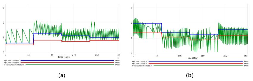
Sustainability 2020, 12, 8920                                                                      6 of 21

                                Figure 3. Factors that affect food requirements. Source: [14].

                                        Figure 4. Feeding decision-making process.

     The main disadvantage of this closed loop approach is that falconers usually do not have sufficient
information to make efficient decisions. This is because such information is limited to the most recent
feeding records. Consequently, airport falconers miss other useful information that could be extracted
from the statistical analysis of a raptor’s past records or from databases pertaining to similar raptor
species, which could be helpful in deciding the best feeding plan to reach the right-hunger point
at a given time. Based on this concept and a previous case study, results after each raptor’s release
could be calculated using allometric equations developed for that purpose [21]. The equations were
calculated for each season in order to provide the first and third quartile of feeding and establish
the upper and lower limits that should lead to the best result when the raptor is released.

2.4. Expected-Result Equations
     The expected-result equations were derived to provide essential information to falconers in order
to plan the feeding of raptors, considering six possible results of their release (see Table 2). For this
purpose, in the first stage of the research, eight raptor specimens (three females and five males; see
Table 3) and their daily feeding records for a period of 10 years (2004–2014) were analyzed, including
their flight evaluation records. Keeping the selected names for the raptors (Niobe, Thirma, Fenix,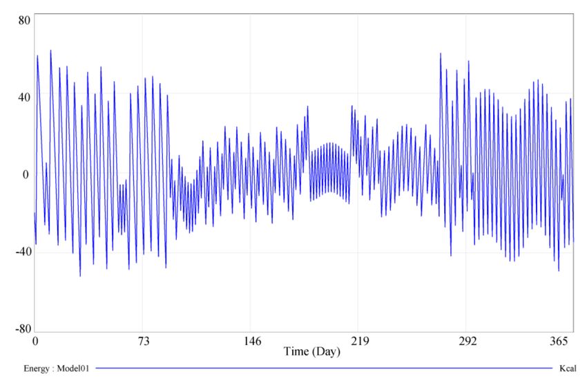
Sustainability 2020, 12, 8920                                                                                  7 of 21

Coz, Titi, Darko, Zeus, and Nico), which expressed the affective bond between raptor and falconer,
a database was built, adding numerical codification to represent each raptor’s gender and specimen
type to aid in reconciling the statistical analysis with the data.

                                             Table 2. Falconer’s evaluation range.

                         Value                                   Description
                            1        Raptor flies but does not return when called
                            2        Bad flight: raptor alights unexpectedly
                                     Regular flight: raptor’s flight height is insufficient; raptor
                            3
                                     does not fly over the entire area
                                     Good flight: raptor will reach the expected height but will
                            4
                                     not fly over the entire area
                            5        Very good: raptor flies over the entire area but returns late
                                     Excellent: raptor’s flight height is sufficient; raptor succeeds
                            6
                                     at hunting and returns when summoned

     The statistical analysis of the records allowed the derivation of equations that could predict
the expected result of a raptor’s release in relation to the feeding factor, which was defined as the ratio
of supplied calories to the raptor’s basal metabolic rate. The equations were calculated following
an exponential structure (see Equation (2)) according to the acceptance criterion of the highest value of
the square of the Pearson product–moment correlation coefficient, R2 .

                                                       ERQi =(a+b·FF)                                             (2)

     Here, ERQi represents the value of the expected result of a raptor release according to the limit value
defined by quartile i (Qi) of feeding factors that corresponded with this result, and a is an independent
term and b the factor that modulates the feeding factor, FF, defined as the coefficient between the calories
supplied by the falconer and the basal metabolic rate of the raptor; see Equation (1).
     These equations were also used to plot the curves marking out the area for the first, second,
and third quartiles, where the feeding factor may generate the best expected result (ER) for the raptor
(ER = 6). The expected-result equations for each raptor are listed in the corresponding tables as well as
for two generic models, considering the gender, where equations for female and male raptors were
created by a new regression of the expected results for each group (see Tables 3 and 4).

                                Table 3. Parameters of Equation (2) for each raptor analyzed.

                                     ERQ3                          ERMed                        ERQ1
            Raptor
                            a          b         R2        a          b        R2       a         b     R2
                         #01HPGH: Female specimen of Falco Rusticolus × Peregrinus (Niobe)
            Winter       −2.02        4.89      0.98     −2.32       5.62      0.96   −2.47      5.97   0.95
            Spring       −1.1         2.64      0.92     −1.74       3.74      0.95   −3.51      6.94   0.92
           Summer        −0.67        1.71      0.98     −0.74       2.31      0.94   −0.92      2.75   0.96
           Autumn        −1.23        2.84      0.93     −1.17       3.02      0.98   −0.84      2.74   0.99
                          #02HSGH: Female specimen of Falco Cherrug × Rusticolus (Thirma)
            Winter       4.12        −3.51      0.99      3.47      −3.19      0.92    1.11     −1.09   0.91
            Spring       −0.76       1.75       0.96     −0.06      1.41       0.97   −0.36     2.15    0.94
           Summer         −2         2.84       0.93     −1.6       3.26       0.92   −1.48     4.16    0.95
           Autumn        −0.85       1.82       0.99     −0.57      1.81       0.91   −0.47     1.93    0.91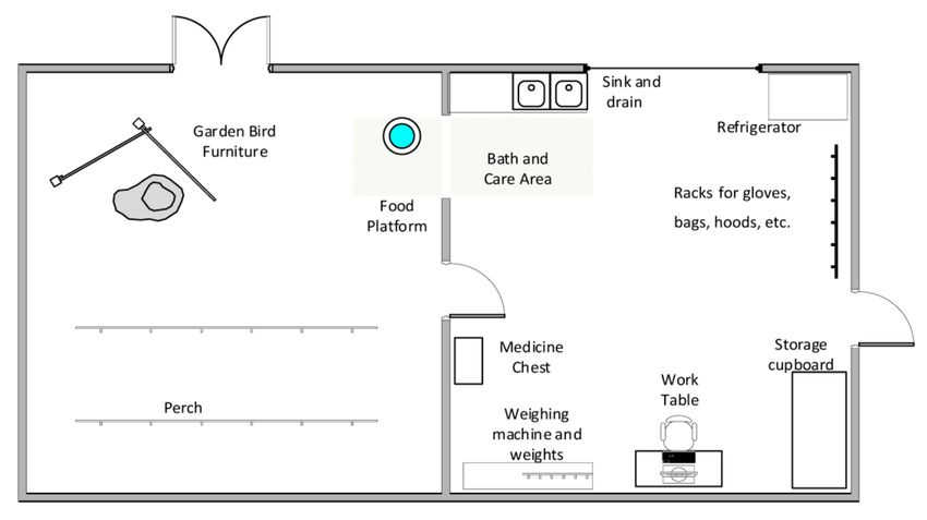
Sustainability 2020, 12, 8920                                                                                8 of 21

                                                      Table 3. Cont.

                                    ERQ3                       ERMed                       ERQ1
            Raptor
                            a          b       R2       a          b      R2        a        b         R2
                          #03HPGM: Male specimen of Falco Rusticolus × Peregrinus (Fenix)
            Winter       10.25       −4.61    0.99    25.77      16.89   0.98     11.17    −7.82      0.99
            Spring        4.16       −1.63    0.91     3.58      −1.62   0.97      2.96    −1.29      0.92
           Summer         3.62       −1.57    0.98     2.88      −1.23   0.95      2.72    −1.29      0.91
           Autumn        −1.66       2.01     0.92    −3.21      3.82    0.98     −5.92    6.95       0.98
                           #04HPGM: Male specimen of Falco Rusticolus × Peregrinus (Coz)
            Winter       −4.05       2.86     0.99    −5.21      3.85    0.98     −5.39    4.96       0.93
            Spring       9.18        −5.72    0.98     9.41      −6.62   0.96     10.99    −8.4       0.94
           Summer        −3.92       4.32     0.90    −5.96      6.31    0.92      5.80    −5.98      0.94
           Autumn        −3.58       3.18     0.99    −7.18      5.86    0.97     −4.67    6.94       0.94
                                    #05HPH: Female specimen of Falco Peregrinus (Titi)
            Winter        2.29        −1      0.99     2.34      −1.34   0.92     2.63     −2.07      0.91
            Spring        7.82       −4.78    0.99     8.81      −6.14   0.95     4.51     −3.67      0.96
           Summer         2.53       −1.25    0.92     2.58      −1.60   0.94     2.75     −2.06      0.94
           Autumn         2.31       −0.97    0.97     2.45      −1.28   0.94     2.30     −1.50      0.94
                          #06HPGM: Male specimen of Falco Rusticolus × Peregrinus (Darko)
            Winter       −0.86       1.14     0.90    −1.13       1.37   0.94    −12.82    10.44      0.97
            Spring       −3.59       2.73     0.93    −7.3        6.00   0.97    −3.36     2.73       0.93
           Summer        −6.08       4.23     0.98    −4.34       3.58   0.92    −2.32     2.52       0.98
           Autumn        −6.67       5.97     0.99    −5.79       5.44   0.94    −10.20     9.94      0.93
                           #07HPGM: Male specimen of Falco Rusticolus × Peregrinus (Zeus)
            Winter       −2.89       2.75     0.99    −4.06      3.70    0.91     −9.84    8.15       0.97
            Spring       5.86        −3.46    0.93     5.81      −3.52   0.99      5.47    −3.41      0.90
           Summer        4.44        −2.23    0.99     4.43      −2.47   0.96      4.31    −2.65      0.97
           Autumn        4.19        −1.83    0.96     6.21      −3.75   0.99      8.12    −5.81      0.94
                               #08HGSM: Male specimen of Falco Cherrug × Rusticolus (Nico)
            Winter       −3.76       2.84     0.95    −6.23      4.74    0.97    −9.33     7.18       0.99
            Spring       2.90        −3.03    0.97     3.28      −1.38   0.92      4.0     −1.98      0.96
           Summer        2.19        −0.62    0.92     2.13      −0.61   0.93     2.09     −0.69      0.99
           Autumn        −4.44       6.46     0.91    −7.50      5.80    0.95    −15.76    12.08      0.98
                                                       Source: [14].

                     Table 4. Parameters of Equation (2) for male/female classification of raptors.

                                    ERQ3                      ERMed                       ERQ1
            Raptor
                           a          b       R2       a          b      R2        a         b        R2
                           Generic modeling prediction of expected results for female raptors
            Winter       3.59       −2.77    0.99    3.68       −3.39    0.97    4.23     −4.95       0.99
            Spring      −3.4         1.19    0.99    −2.37       3.67    0.99   −5.62      8.89       0.99
            Summer      −22.6       21.74    0.99    −21.3      26.45    0.99   −17.04    25.25       0.99
            Autumn      24.92       −22.7    0.99    −18.1      21.45    0.95   −9.76     14.03       0.99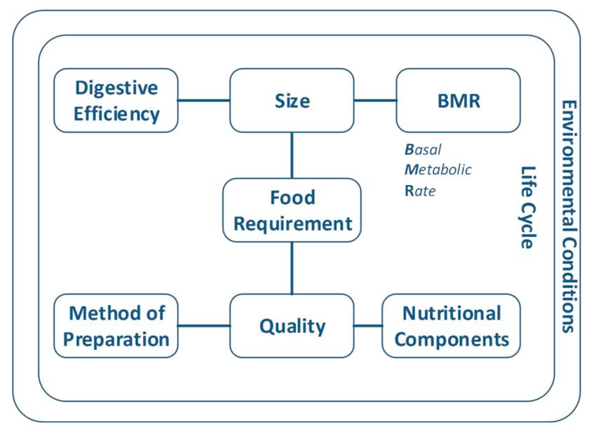
Sustainability 2020, 12, 8920                                                                           9 of 21

                                                     Table 4. Cont.

                                 ERQ3                        ERMed                       ERQ1
            Raptor
                           a        b       R2        a          b      R2        a        b     R2
                            Generic modeling prediction of expected results for male raptors
            Winter      −3.92     2.91      0.99    −4.31      3.5     0.97    −13.58    10.93   0.99
            Spring       5.92     −3.0      0.99      5.5      −3.1    0.92     4.98     −2.93   0.99
            Summer       4.59     −2.62     0.99     4.07      −2.1    0.99     3.72     −2.14   0.99
            Autumn      −9.18     6.99      0.91    −10.75     9.58    0.95    51.14     −41.6   0.98
                                                      Source: [14].

3. Proposed Dynamic System
     The nutritional balance required to lead raptors to reach the right-hunger point can be understood
as a dynamical system. Falconers adjust the food input to control the raptors’ weight to lead them to
right-hunger status. It is analogous to the process of filling a water tank (Figure 5) with two drainage
lines at the bottom: one line is for calories that satisfy the energy requirement to survive and perform
daily activities, and the other for calories that are used to increase the raptor´s weight. Controlling
the water tap represents feeding the raptor, and the tank level represents the energy modulated by
the raptor that will be used to satisfy the basal metabolic rate plus the exercise energy requirements,
transforming excess energy into fat, which in turn increases the raptor’s weight.

                                 Figure 5. Dynamic system: water filling tank analogy.

      Falconers, acting as decision-makers regarding the amount of food to be assigned, have to know
the daily weight of each raptor in order to calculate the basal metabolic rate and contrast it with
the input of calories. This ratio between caloric input and required minimum is commonly called
the feeding factor. Hence, a ratio less than 1 means that the falconer decided to reduce the raptor’s
weight, and a ratio greater than 1 means that the falconer opted to increase it. The basal metabolic rate
is calculated by an allometric equation that depends on weight, whereas the caloric input is obtained
by a food subsystem that determines the equivalent calorie counts of food items. The expected results
can be quickly obtained by using an equation that depends on the feeding factor.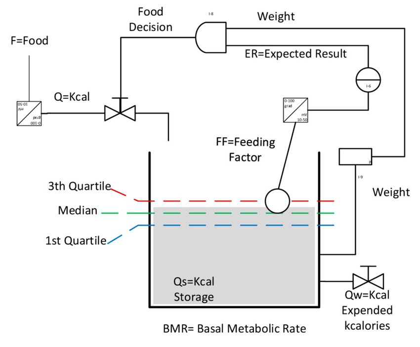
Sustainability 2020, 12, 8920                                                                        10 of 21

      Variable Characterization

•     Food: This is an independent and qualitative variable defined by the nutritional items the falconer
      supplies to the raptor. Food items are usually day-old chicks or chicken wings, thigh, or breast
      portions. Professional falconers source them from food raptor farms, which allow the tracking of
      nutritional information for each food item.
•     Q: This parameter, which is dependent on the food variable, is a quantitative and continuous
      variable that represents the calories supplied by each food input. The food transformation system
      transduces the food variable into a numerical value that represents the energy (calories) supplied
      to the raptor (Table 5).
•     Weight: Initially, this is an independent variable. In the model design, it becomes a dependent
      variable for stored and consumed energy; it is a quantitative and continuous variable that
      represents the weight of a raptor expressed in kg.
•     FF: This is a dependent variable that represents the feeding factor by means of the ratio of Q to
      BMR: FF = Q/BMR; it is a quantitative and continuous variable.
•     Season: This variable is dependent on time. It is a qualitative and discrete variable that represents
      the seasonal effects when modelling raptor behavior and nutritional needs.
•     ER: This variable, which is dependent on FF and season, is a quantitative and discrete variable
      (between 1 and 6) that evaluates the release of the raptor, with 1 representing the worst possible
      result and 6 the best possible result (Table 2).
•     BMR: This variable, which is dependent on weight, is a quantitative and continuous variable.
      The basal metabolic rate expresses the minimum number of calories that the raptor requires to
      survive (assuming it remains in a resting state), (see Equation (1)) [27].

                                              Table 5. Food–calorie conversion.

                                  Food Description                          kcal/Unit
                                   Day-old chicks                              39.6
                                Chicken wing portion                           57.96
                                Chicken breast portion                         38.22
                                 Extracted from nutritional descriptions of Labdial food supplier.

3.1. Simulation Software Implementation
     Industrial-strength simulations can help improve an airport falconer’s decision-making capacity
by implementing a dynamic system that can be used to obtain a feeding baseline plan associated with
the best expected result. In order to set up this type of simulation, Vensim is suitable software that
allows the creation of a dynamic model to run the required iterations for the final result. This software
offers a simple interface to design a high-quality model, data connections, flexible distribution,
and advanced algorithms.
     The model design is similar to the conventional problem of water tank filling (Figure 6), in which
there is an input of calories to feed the raptor and a minimum caloric energy required for the raptor to
survive, plus additional energy for the hunting flight. The tank-level objective is defined by the feeding
factor that leads to the best result, that is, the limits defined by the first and third percentiles of
the feeding factor that were previously obtained by the expected model for each raptor.
Sustainability 2020, 12, 8920 11 of 21
Figure 6. Proposed dynamic system designed with Vensim software.
The stored energy can be converted into a weight-change ratio by means of a statistical analysis
performed in previous research showing that for each kilocalorie supplied a day before weighing, it
can be assumed that the weight will increase by 0.1 g. This conversion ratio is the reference value
considered in this research, where several assumptions were made, and it may not be correct to
extrapolate them to other case studies with different boundary conditions. The seasonal component
affects not only the expected result, but also the energy consumption, because of the raptor’s daily
activities. This can be expressed in terms of BMR: 0.2 times the BMR for winter, 0.25 for spring, 0.3 for
summer, and 0.25 for autumn, as reported by international studies [28,29].
3.2. Vensim Variables
Vensim software uses different types of variables, such as level, auxiliary, data, constant, lookups,
and arrows, including an equation editor, in order to display the internal relationships between them.
In this case, the water tank analogy is an aid to understanding how raptor modeling uses level variables
such as energy and weight as storage capacity that represents a level for accumulating positive or
negative inputs, which can increase or decrease their initial values.
Auxiliary variables perform an important function; sometimes the main purpose is to provide easy
access to an intermediate operation value in order to clearly plot its effects on the process. For example,
the New variable is used to add the value of the Diet variable to the baseline food plan that corresponds
to the Food variable.
The rest of the variables are summarized in Table 6. These variables play a part in the three main
loops that combine them in groups of four, six, and seven steps per loop. The first loop depends
on the variables Weight, Consumption, Energy, and Nutrition; the second loop depends on Weight,
BMR, Feeding Factor, Index, Diet, Energy, and Nutrition; and the third loop depends on Weight,
BMR, Consumption, Feeding Factor, Index, Diet, Energy, and Nutrition. Feeding Factor is therefore
influenced by Energy, BMR, and Consumption; Diet is influenced by Index, which depends on Feeding
Factor, Q3Limit, and Q1Limit; and Consumption is defined by BMR and Energy Release Factor, all of
which are represented more clearly because of the causal tree that characterizes the Vensim model
(Figure 7).Sustainability 2020, 12, 8920 12 of 21
Figure 7. Causal trees for most relevant variables: (a) feeding factor, (b) diet, and (c) consumption.
Table 6. Variables used in Vensim.
Variable Description Unit
Auxiliary variable to express basal metabolic rate.
BMR kcal
Auxiliary variable that represents nutritional
variation. This variation on the planned standard
food depends on the Index variable. , where α,
β, and γ are calories (kcal) of standard portions of
food most commonly used to increase or decrease
the diet (Table 7).
Level of stored energy.
Auxiliary variable that expresses standard feeding
plan (in kcal), estimated by means of case study
Food kcal
analysis; most commonly 150 kcal.
Auxiliary variable indicating that if feeding factor is
over Q3 limits, its value is −1; if between Q3 and Q1
limits, its value is 0.5; if under Q1 limits, its value is
Index +1. Q3Limit, −1,0) + IF THEN
ELSE(Feeding Factor < Q1Limit,1,0)>>
Auxiliary variable for new feeding input.
Auxiliary variable that represents weight variation
caused by energy balance between calorie supply
Nutrition kg
and energy consumption.Sustainability 2020, 12, 8920 13 of 21
Table 6. Cont.
Variable Description Unit
Lookup variable that represents seasonal effects on
Performance daily activity.
Auxiliary variable that represents upper limit of
Q3Limit feeding factor (third quartile) that can lead raptor to Dml
a successful flight.
Auxiliary variable that represents lower limit of
Q1Limit feeding factor (first quartile) that can lead raptor to Dml
a successful flight.
Lookup variable that contains Q3 limits for different
raptor models. Models 01–08 correspond to species
Q3model and gender, models 09 and 10 are for female Dml
and male median values, respectively.
Lookup variable that contains all Q1 limits for
different raptor models. Models 01–08 correspond to
species and gender, models 09 and 10 are for female
Q1model Dml
and male median values, respectively.
Auxiliary variable: 1 for winter, 2 for spring, 3 for
summer, 4 for autumn. >
Shadow variable used to set timing.
Auxiliary variable for total energy consumed, defined
Consumption by BMR and energy needed to accomplish raptor’s kcal
activity.
Level variable with an initial value introduced for
each simulation; e.g., for a simulation of a young
Weight kg
raptor, the initial weight is 0.8 kg.
Auxiliary variable that is a factor to be multiplied by
Release Energy BMR and added to Consumption. Represents energy
Dml
Factor that will be consumed because of raptor activity.
Dml, dimensionless.
Table 7. Variation parameters (in kcal) of standard portions of food for each model.
Model: 01 02 03 04 05 06 07 08 Female Male
α −90 −90 −90 −90 −90 −90 −90 −90 −90 −50
β −20 −20 −20 −20 −20 −40 −20 −20 −20 10
γ 30 30 30 30 80 10 30 30 30 50
Food 150 150 100 100 150 100 100 100 170 100
3.3. Vensim Simulations
Simulations were performed for each model, that is, for each raptor selected, including all
the years of their existing records in the database. As the model is limited to a step time of one year,
the simulations were repeated for each year using the actual value recorded at the beginning of the year
as the initial weight.Sustainability 2020, 12, 8920 14 of 21
Finally, a new database was obtained for each raptor (models 01–08). In order to test the Vensim
model’s reliability (such as in the other examples), hindcasting was performed by checking whether
the model output corresponded to the forecasted values, and whether validation data corresponded to
observations [30]. This made it easy to compare several models by examining the mean square error
(see Equation (3)) or the symmetric mean absolute percentage error (see Equation (4)) as a modification
of this error when the divisor is half the sum of the actual and forecast values [31].
Thus, for each raptor, three models were compared with the developed model: the generic
model that depends on the raptor’s gender, the falconer behavior that modulates the feeding factor,
and the actual feeding plan designed by the falconer. The validation data represent the third percentile
value of the feeding factor for each season that leads the raptor to a successful flight when released.
The equations used are as follows:
n
1 X 2
MSE = Yi − Ŷi (3)
n
i=1
where Ŷi is a vector of n-predictions and Yi is the vector used as a reference; and
n
1 X |Ft − At |
SMAPE =
Ft +At
(4)
n
t=1 2
where Ft is the forecast value obtained with Vensim and At is the value used as a reference.
In both cases the reference value corresponded with the feeding factor (FF) from Equation (2) for
the highest possible result (ER = 6), applying the values in Table 3 for each case. The prediction vectors
and forecast values were the FF obtained with Vensim modeling, and the falconer trial-and-error
output labelled “Actual Observed” and “M/F Model” was the FF from Equation (2) for the highest
possible result (ER = 6), applying values in Table 4 for each case.
4. Results and Discussion
4.1. Simulation Results and Graphical Information
Vensim software allows simulation results to be configured in several ways. This can be in tables,
diagrams, graphics, or exportable files in .csv or .txt format that may be of interest in order to subsequently
perform statistical analysis on the results. Figures 8 and 9 show examples of results that were obtained
from the Vensim simulations. Figure 8 represents the energy balance that produces a weight increase or
reduction, and Figure 9 represents the forecast vs. actual weight for the time frame selected for a female
specimen of Falco rusticolus peregrinus (raptor #01HPGH).
The feeding factor results, listed in a table format, provide the numerical information that
the falconer can use to determine an initial feeding baseline in order to keep the raptor feeding between
the first and third percentile limits; these limits may lead to the best results when the raptor is released.
As for the weight forecast, Figure 9 shows how Vensim modeling offers a smooth forecast of the raptor’s
weight. This could be used by airport falconers as a baseline to set new feeding objectives from one
year to the next. However, forecasting weight is a difficult research problem because all the nutritional
components should be analyzed in order to accept forecast values. Thus, the feeding factor was used
as a control parameter to set new feeding objectives, because it refers to a basal metabolic rate that
depends on the actual weight of the raptor.Sustainability 2020, 12, 8920 15 of 21
Figure 8. Example of energy balance forecast result for model 01, raptor #01HPGH.
Figure 9. Weight forecast vs. actual weight for model 01, raptor #01HPGH, applied to 2011.
Therefore, the feeding factor allows the use of a dependent reference variable that can be easily
adjusted by airport falconers by applying their own conversion tables of food into calories instead of
using the list in Table 5.
The feeding forecast is a dynamic system where the first and third percentile limits provide a range
of values in which the feeding should be set by the falconer as a goal. It is difficult to achieve the exact
value of the feeding factor because food is supplied in full or partial portions of standard items. This
aspect is introduced into the simulation by defining the most common responses of falconers (Table 6)
to a diet variation when the feeding factor is over the third percentile (Q3), between the third and first
percentiles (inside the Q3–Q1 interval), or below the first percentile (Q1).
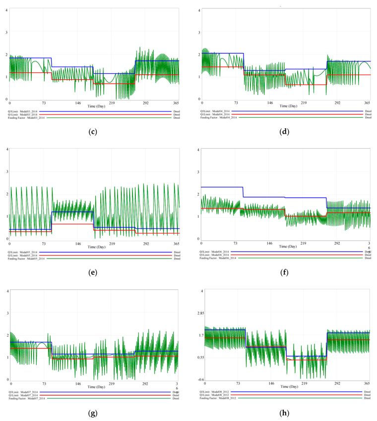
This circumstance explains why the feeding factor variance increases when its limits (Q3–Q1)
are considerably close in value (Figures 10 and 11). As for the reliability of simulations, results were
compared with the actual information recorded by the falconer from 2004 to 2014. This made it
possible to determine the mean squares and symmetric mean absolute percentage errors by analyzingSustainability 2020, 12, 8920 16 of 21
the differences between the forecast feeding factor and the feeding factor that can lead to the best
results for each raptor when released, referring to the third percentile.
Figure 10. Feeding factor plots for models 01–08: (a) raptor #01HPGH; (b) raptor #02HSGH; (c) raptor
#03HPGM; (d) raptor #04HPGM; (e) raptor #05HPH; (f) raptor #06HPGM; (g) raptor #07HPGM; (h)
raptor #08HGSM.Sustainability 2020, 12, 8920 17 of 21
Figure 11. Feeding factor plot according to raptor gender: (a) female and (b) male.
4.2. Simulation Reliability Results
The mean square error is a statistical indicator that penalizes higher differences between forecast
and actual values. The symmetric mean absolute percentage error is a statistical indicator that can be
used to contrast forecast models even though it is not a fully symmetric method, because the upper
and lower values in the forecast are not treated equally. Rather than characterizing the Vensim model
error, these indicators were used to identify the model that would fit better as a forecast model of
the raptor’s feeding process; therefore, the error value must be understood as a relative value used to
compare models for a specific raptor and a generic model based on the raptor’s gender. The results are
summarized in Table 8. The mean square error (MSE) for the models designed with Vensim for each
raptor was always lower than that obtained from actual observations of the airport falconer. Thus, it
could be assumed that the Vensim model for each raptor can improve the falconer’s decision-making
process regarding the feeding factor.
Table 8. Results of mean squared error (MSE) and symmetric mean absolute percentage error (SMAPE).
Model MSE * (Referring to Q3) SMAPE * (Referring to Q3) SMAPE ** (Referring to Q3)
(i) A B C A B C A B C
01 0.1719 0.4812 0.1986 28.37% 46.36% 29.09% 31.82% 49.65% 32.12%
02 0.1093 0.4187 0.1301 24.68% 45.23% 28.61% 27.58% 52.90% 30.82%
03 0.2570 0.2969 0.2848 34.16% 37.44% 35.70% 48.86% 53.95% 51.28%
04 0.2519 0.3120 0.3050 32.62% 35.22% 33.72% 44.73% 47.96% 46.11%
05 0.6594 0.7110 0.5506 57.84% 66.39% 61.26% 66.34% 70.48% 63.90%
06 0.5516 0.7076 0.6688 46.21% 52.91% 51.38% 54.29% 67.96% 63.72%
07 0.2670 1.2907 0.2981 38.29% 53.93% 46.68% 50.31% 62.05% 55.48%
08 0.2595 0.5807 0.2777 35.86% 42.85% 37.74% 38.90% 49.29% 47.58%
A: Forecast vector was FF values obtained with Vensim model. B: Forecast vector was formed by FF values recorded
by falconer using a trial-and-error system. C: Forecast vector was set with FF values from Equation (2) for ER =
6 applying values from Table 4 in each case. Reference vector corresponded to FF from Equation (2) for ER = 6
applying values from Table 3 in each case. * Includes all data; ** excludes data inside interval [Q1,Q3].
The generic model that depends on the raptor’s gender also provided a lower MSE than actual
observations, which can be used for new case studies that do not have sufficient data to design a specific
model. The models, except model 05, yielded a lower MSE compared to a reference generic model.
The MSE of the generic and specific models was 0.5506 and 0.6594, respectively. The reason for this
was that model 05 represented a young raptor that was in a growing trend instead of a conventional
activity. This motivated the falconer to increase the raptor’s weight with increased feeding, which
resulted in a bigger input of calories into the Vensim model beyond the required input (Table 7).
Although error comparison is a valid method to set acceptance criteria to determine which model
fits better with actual values referred to in the Q3 limit (previously calculated), there could be several
forecast values noted as errors, even though these may be within the acceptance interval [Q1,Q3].Sustainability 2020, 12, 8920 18 of 21
Therefore, to determine the symmetric mean absolute percentage error (SMAPE), two sets of values
were calculated: SMAPE values of all databases that conformed with all forecast values, and SMAPE
values of forecast databases in which feeding factors within the interval [Q1,Q3] were removed.
Table 8 summarizes SMAPE * results, which correspond with the symmetric mean absolute
percentage error calculated by considering the value of the third percentile of the feeding factor that
yielded the best result for the raptor´s release. The list also includes SMAPE **, which corresponds
with the symmetric mean absolute percentage error calculated only for feeding forecast values outside
the interval [Q1,Q3]. It can be observed that the lowest value of SMAPE * was 24.68%, corresponding
to model 02, which was designed for a female specimen of Falco cherrug rusticolus. The highest
value was 57.84%, corresponding to model 05, which was designed for a female specimen of Falco
peregrinus. The same trend is observed for SMAPE **, with values of 27.58 and 66.04% for models 02
and 05, respectively.
These results reveal that in all cases, specific models had lower error percentages than the falconer’s
actual observations. This further confirms that the Vensim model can be used to define a feeding
factor baseline to lead raptors to the right-hunger point. Moreover, this shows that generic models
that depend on raptor gender are suitable for forecasting when records are not sufficient to perform
statistical studies to design specific models.
5. Conclusions and Future Research
The aim of this research was to provide a baseline for the raptor feeding factor for airport falconry
in order to aid falconers in the decision-making process to lead raptors to the right-hunger point
and keep them there. A dynamic system was designed based on an analogy with the water tank filling
problem, where several feedback inputs allow control of feeding the raptor according to an interval
defined by the first and third percentile of the feeding factor, which would lead the raptor to succeed
when released.
The simulations performed allowed this baseline to be defined in a one-year framework, which
could be easily updated to obtain new forecast values of the feeding factor. To this end, Vensim
software, with its user-friendly interface, proved to be a useful tool to set all required parameters
in the analysis. However, several raptor species could not be simulated because certain features of
the case study did not include all types of raptors that can be used in airport falconry.
Even though this research did not analyze other case studies, it opens new research lines where
these results may be considered in relation to other airport features that may affect the feeding process;
consequently, adjustments to improve the results may be proposed. This perspective is deemed
relevant, because in the early stage of this research, a strategic communication model was proposed to
allow knowledge transfer among airport falconers through record sharing (Figure 12).
The developed Vensim model can be freely shared with other airport falconers as a key to unlock
the transfer of knowledge acquired from this study. Accordingly, a new study that includes new
parameters, such as the wildlife impact ratio per 100,000 operations (as defined by the International
Civil Aviation Organization), could be initiated [32]. This could encourage airport stakeholders to
analyze other case studies where the information obtained from this study could be used to investigate
new ways of evaluating the efficiency of airport falconry activities following a risk property-based
classification and big data analysis [33] alongside new ways of pattern recognition within big data
processes [34]. In addition, incoming research lines with regard to finding the right-hunger point
in addition to the best expected behavior of raptors when they are released can take advantage
of new solutions for the decision problem using fuzzy problem solving, such as by fuzzy Laplace
transforms [35], which could extend the research scope of this paper.
Furthermore, the feeding factor forecast opens a new cross-research opportunity by considering
logistical studies regarding food acquisition for raptors and the use of traceable food supplier data,
which could help airport falconers to optimize the food request process by minimizing delivery time
and transport cost.Sustainability 2020, 12, 8920 19 of 21
Figure 12. Comparison between (a) actual and (b) proposed system design for airport falconry.
Author Contributions: Conceptualization, J.L.R.-G.; methodology, J.L.R.-G. and F.C.-B.; software, F.C.-B.;
validation, J.L.R.-G. and A.J.B.P.; formal analysis, A.J.B.P.; investigation, J.L.R.-G. and A.J.B.P.; resources, J.L.R.-G.
and A.J.B.P.; data curation, J.L.R.-G. and F.C.-B.; writing—original draft preparation, J.L.R.-G.; writing—review
and editing, A.J.B.P. and F.C.-B.; supervision, J.L.R.-G. All authors have read and agreed to the published version
of the manuscript.
Funding: This research received no external funding.
Acknowledgments: The authors would like to express their sincere gratitude to Desheng Wu from the University
of the Chinese Academy of Sciences and Stockholm University, whose comments helped to improve this
paper considerably.
Conflicts of Interest: The authors declare no conflict of interest.
References
1. Dolbeer, R.A.; Wright, S.E.; Weller, J.; Begier, M.J. Wildlife Strikes to Civil Aircraft in the United States,
1990–2014. no. Serial Report Number 15, 2014. Available online: https://rosap.ntl.bts.gov/view/dot/6461
(accessed on 4 December 2016).
2. Allan, J.R. The cost of bird strikes and birdstrike prevention. In Human Conflicts with Wildlife: Economic
Considerations; National Wildlife Research Cener: Fort Collins, CO, USA, 2000; Volume 1, pp. 147–153.
Available online: https://digitalcommons.unl.edu/nwrchumanconflicts/18 (accessed on 12 March 2014).
3. Anderson, A.; Carpenter, D.S.; Begier, M.J.; Blackwell, B.F.; DeVault, T.L.; Shwiff, S.A. Modeling the cost of
bird strikes to US civil aircraft. Transp. Res. Part Transp. Environ. 2015, 38, 49–58. [CrossRef]
4. Schwarz, K.B.; Belant, J.L.; Martin, J.A.; DeVault, T.L.; Wang, G. Behavioral traits and airport type affect
mammal incidents with U.S. civil aircraft. Environ. Manag. 2014, 54, 908–918. [CrossRef]
5. Hesse, G.; Rea, R.V.; Booth, A.L. Wildlife management practices at western Canadian airports. J. Air Transp.
Manag. 2010, 16, 185–190. [CrossRef]
6. Blackwell, B.; DeVault, T.; Fernández-Juricic, E.; Dolbeer, R. Wildlife collisions with aircraft: A missing
component of land-use planning for airports. Landsc. Urban Plan. 2009, 93, 1–9. [CrossRef]
7. Zugasti, M. Birds at Airports: The Use of Falconry, 4th ed.; Aena Aeropuertos, S.A.: Madrid, Spain, 2008;
ISBN 9788496456884.
8. Cook, A.; Rushton, S.; Allan, J.; Baxter, A. An Evaluation of Techniques to Control Problem Bird Species on
Landfill Sites. Environ. Manag. 2008, 41, 834–843. [CrossRef] [PubMed]
9. Yang, D.-D.; Zhang, Z.-Q.; Hu, M.-W. Ranking birdstrike risk: A case study at Huanghua International
Airport, Changsha, China. Acta Ecol. Sin. 2010, 30, 85–92. [CrossRef]
10. Kitowski, I.; Grzywaczewski, G.; Cwiklak, J.; Grzegorzewski, M.; Krop, S. Falconer activities as a bird
dispersal tool at Deblin Airfield (E Poland). Transp. Res. Part Transp. Environ. 2011, 16, 82–86. [CrossRef]Sustainability 2020, 12, 8920 20 of 21
11. Blackwell, B.F.; Seamans, T.W.; Schmidt, P.M.; Vault, T.L.D.; Belant, J.L.; Whittingham, M.J.; Martin, J.A.;
Fernández-Juricic, E. A framework for managing airport grasslands and birds amidst conflicting priorities.
Ibis 2013, 155, 199–203. [CrossRef]
12. Ning, H.; Chen, W. Bird strike risk evaluation at airports. Aircr. Eng. Aerosp. Technol. Int. J. 2014, 86, 129–137.
[CrossRef]
13. Matyjasiak, P. Methods of bird control at airports. In Theoretical and Applied Aspects of Modern Ecology;
Wydawnictwo Uniwersytetu Kardynala Stefana Wyszynskiego: Warsaw, Poland, 2008; Volume 1, pp. 171–203.
ISBN 978-83-7072-562-4.
14. Roca-González, J.L.; Vera López, J.A.; Fernández Martínez, M. Raptor’s “Right Hunger” Characterization to
Develop Sustainable Exclusion Areas for wildlife at Civil & Military Airports. Appl. Math. Nonlinear Sci.
2016, 1, 335–344. [CrossRef]
15. Staton, D. An Analysis of Australian Birdstrike Occurrences 2002 to 2006; Safety publications, Australian
Transport Safety Bureau: Camberra City, Australia, 2008; p. 139. Available online: https://www.atsb.gov.au/
publications/2008/ar2008027/ (accessed on 27 February 2020).
16. Thiériot, E.; Patenaude-Monette, M.; Molina, P.; Giroux, J.-F. The Efficiency of an Integrated Program Using
Falconry to Deter Gulls from Landfills. Animals 2015, 5, 214–225. [CrossRef] [PubMed]
17. Littauer, G.; Glahn, J.; Reinhold, D.; Brunson, M.; Brunson, M.; Brunson, M. Control of Bird Predation at
Aquaculture Facilities: Strategies and Cost Estimates; SRAC Publication, Southern Regional Aquaculture Center:
Stoneville, MS, USA, 1997.
18. Clark, L.; Shivik, J.A.; Watkins, R.A.; VerCauteren, K.T.; Yoder, J.K. Human Conflicts with Wildlife:
Economic Considerations. In Proceedings of the National Wildlife Research Center Symposium, Fort
Collins, CO, USA, 1–3 August 2000; Available online: https://digitalcommons.unl.edu/nwrchumanconflicts/
(accessed on 27 February 2020).
19. Wilke, S.; Majumdar, A.; Ochieng, W.Y. A framework for assessing the quality of aviation safety databases.
Saf. Sci. 2014, 63, 133–145. [CrossRef]
20. Tvrdon, L.; Fedorko, G. Usage of Dynamic Simulation in Pressing Shop Production System Design. Int. J.
Simul. Model. 2020, 19, 185–196. [CrossRef]
21. Roca-Gonzalez, J.-L. Designing dynamical systems for security and defence network knowledge management.
A case of study: Airport bird control falconers organizations. Discrete Contin. Dyn. Syst.-S 2015, 8, 1311.
[CrossRef]
22. International Civil Aviation Organization. Airport Services Manual Part 3 Wildlife Control and Reduction, 4th ed.;
International Civil Aviation Organization: Montréal, QC, Canada, 2012; ISBN 978-92-9231-929-8.
23. Burger, J. Bird Control at Airports. Environ. Conserv. 1983, 10, 115–124. [CrossRef]
24. Ceballos, J.; Justribó, J.H. Manual Básico y Ético de Cetrería; Avium: Madrid, Spain, 2011;
ISBN 978-84-85707-63-8.
25. Ferguson-Lees, J.; Christie, D.A. Raptors of the World; Houghton Mifflin: Boston, MA, USA, 2001;
ISBN 978-0-618-12762-7.
26. Glasier, P. Falconry and Hawking; Charles Branford Publisher: London, UK, 1986; ISBN 978-07-13455557.
27. Sedgwick, C.J.; Haskell, A.; Pokras, M. Scaling drug dosages for animals of diverse body sizes. Wildl.
Rehabilators 1986, 5, 3–11.
28. Porkas, M.; Karas, A.; Kirkwood, J.; Sedgwick, C.J. An introduction to allometric scaling and its uses in raptor
medicine. In Raptor Biomedicine; University of Minesota Press: Minneapolis, MN, USA, 1993; Volume 37,
pp. 211–228.
29. Barton, N.W.H.; Houston, D.C. A comparison of digestive efficiency in birds of prey. Ibis 1993, 135, 363–371.
[CrossRef]
30. Morley, S.K.; Brito, T.V.; Welling, D.T. Measures of Model Performance Based On the Log Accuracy Ratio.
Space Weather 2018, 16, 69–88. [CrossRef]
31. Kim, S.; Kim, H. A new metric of absolute percentage error for intermittent demand forecasts. Int. J. Forecast.
2016, 32, 669–679. [CrossRef]
32. Roca-González, J.-L.; Vera-Lopez, J.-A.; Rodriguez-Bermudez, G. Organisational and costing aspects to
prevent wildlife strikes on airports: A case study of Spanish airport security managers. Saf. Sci. 2020, 122,
104520. [CrossRef]Sustainability 2020, 12, 8920 21 of 21
33. Wu, D.; Birge, J.R. Risk Intelligence in Big Data Era: A Review and Introduction to Special Issue. IEEE Trans.
Cybern. 2016, 46, 1718–1720. [CrossRef]
34. Xie, T.; Liu, R.; Wei, Z. Improvement of the Fast Clustering Algorithm Improved by K-Means in the Big Data.
Appl. Math. Nonlinear Sci. 2020, 5, 1–10. [CrossRef]
35. Çitil, H.G. Investigation of A Fuzzy Problem by the Fuzzy Laplace Transform. Appl. Math. Nonlinear Sci.
2019, 4, 407–416. [CrossRef]
Publisher’s Note: MDPI stays neutral with regard to jurisdictional claims in published maps and institutional
affiliations.
© 2020 by the authors. Licensee MDPI, Basel, Switzerland. This article is an open access
article distributed under the terms and conditions of the Creative Commons Attribution
(CC BY) license (http://creativecommons.org/licenses/by/4.0/).You can also read