Lightweight Contextual Ranking of City Pictures: Urban Sociology to the Rescue
←
→
Page content transcription
If your browser does not render page correctly, please read the page content below
Lightweight Contextual Ranking of City Pictures: Urban Sociology to the Rescue

  Vinicius Zambaldi †                 Joao Paulo Pesce †                 Daniele Quercia ‡                 Virgilio Almeida †
  fzvinicius@dcc.ufmg.br                jpesce@dcc.ufmg.br                 dquercia@acm.org                 virgilio@dcc.ufmg.br

                                              † Universidade Federal de Minas Gerais, Brazil
                                                     ‡ Yahoo Labs, Barcelona, Spain

                           Abstract                                        To complement those solutions (largely meant for the
                                                                        web), we set out to consider a key element that has been
  To increase mobile user engagement, photo sharing sites are
  trying to identify interesting and memorable pictures. Past
                                                                        hitherto left out: the idea of neighborhood. Pictures taken
  proposals for identifying such pictures have relied on either         in a neighborhood reflect the neighborhood itself and peo-
  metadata (e.g., likes) or visual features. In practice, tech-         ple’s idea of it. Since urban sociology has already dealt
  niques based on those two inputs do not always work: meta-            with those psychological aspects, we use prominent ur-
  data is sparse (only few pictures have considerable number of         ban theories that aimed at explaining, for example, why a
  likes), and extracting visual features is computationally ex-         neighborhood is recognizable and distinctive (Lynch 1960;
  pensive. In mobile solutions, geo-referenced content becomes          Milgram, Kessler, and McKenna 1972), and why it is per-
  increasingly important. The premise behind this work is that          ceived to be beautiful, quiet, and happy (Peterson 1967). In
  pictures of a neighborhood are related to the way the neigh-          so doing, we make the following main contributions:
  borhood is perceived by people: whether it is, for instance,
  distinctive and beautiful or not. Since 1970s, urban theories         • We gather geo-referenced Flickr pictures and contextual
  proposed by Lynch, Milgram and Peterson aimed at systemat-              variables (e.g., weather conditions) in the city of London
  ically capturing the way people perceive neighborhoods. Here            (Section 3).
  we tested whether those theories could be put to use for au-
  tomatically identifying appealing city pictures. We did so by         • We identify six main qualities that describe the way a
  gathering geo-referenced Flickr pictures in the city of Lon-            city is psychologically perceived (Section 4) and quantify
  don; selecting six urban qualities associated with those urban          those qualities using proxies computed from Flickr and
  theories; computing proxies for those qualities from online             Foursquare data (Section 5).
  social media data; and ranking Flickr pictures based on those
  proxies. We find that our proposal enjoys three main desirable        • We rank Flickr pictures based on those proxies and find
  properties: it is effective, scalable, and aware of contextual          that such a ranking enjoys three main desirable proper-
  changes such as time of day and weather condition. All this             ties (Section 6). First, it is effective, in that, the ranked
  suggests new promising research directions for multi-modal              results are similar yet complementary to the results pro-
  learning approaches that automatically identify appealing city          duced by existing metadata-based solutions. Second, it is
  pictures.                                                               computationally inexpensive and, as such, scalable: our
                                                                          proxies are defined at the level of city rather than of pic-
                     1    Introduction                                    ture and can be computed offline (no need for real-time
                                                                          updates). Third, it is aware of contextual factors (Section
To offer an engaging mobile experience, photo sharing                     7): different values of the same proxy can be computed
sites are trying to identify interesting and memorable geo-               as a function of, for example, the time of day or weather
referenced pictures. To determine which pictures are inter-               condition.
esting and memorable, researchers have heavily explored
web-based solutions based on either metadata (e.g., likes) or              As we shall conclude in Section 8, these results suggest
visual features, or the combination of both. The main idea is           that, to offer a better mobile experience, future multi-modal
that interesting pictures are those that have received a con-           learning research should further explore the idea of combin-
siderable number of likes or that contain the visual cues peo-          ing traditional features with domain-specific ones.
ple often perceive to be beautiful.
   Unfortunately, as we shall see in Section 2, metadata hap-                                  2   Related Work
pens to be sparse (only few pictures have considerable num-             To identify the pictures users tend to like, researchers have
ber of likes), and visual extraction is computationally ex-             often used metadata. This is generally of two types. The first
pensive and needs to be augmented with additional classes               is textual metadata and is the most widely used: it consists
of features to guarantee good levels of accuracy.                       of comments and tags users have annotated a picture with
Copyright c 2014, Association for the Advancement of Artificial         (van Zwol, Rae, and Garcia Pueyo 2010). The second type
Intelligence (www.aaai.org). All rights reserved.                       of metadata consists of social features and has received less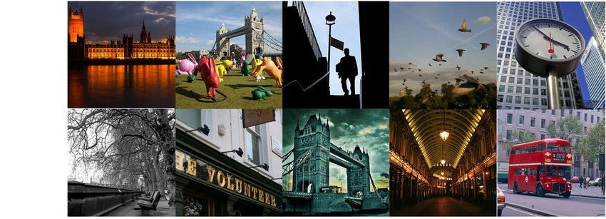
attention. van Zwol et al., for example, used the commu-
nication and social network of Flickr users for predicting
the number of likes (favorites) a picture has received (van
Zwol, Rae, and Garcia Pueyo 2010). They found that social
features alone yielded a good baseline performance, but the
addition of textual features resulted in greatly improved pre-
cision and recall.
   Despite showing good accuracies, approaches that rely
on metadata suffer from coverage. That is because the fre-
quency distributions of tags, comments, or any other social
feature are power law: few pictures are heavily annotated,
while many have little (if any) annotation (Sigurbjörnsson
and van Zwol 2008). As such, approaches solely relying on
metadata do not work for most of the pictures.
   In those situations, researchers have explored the use of
visual categorization. The most effective method is called
bag-of-word model (Datta et al. 2006). This computes de-
scriptors at specific points in an image. It has been shown
that, given an image’s descriptors, machine learning algo-         Figure 1: London Density Map of Photos in our Dataset.
rithms are able to predict whether people tend to find the
image interesting and appealing (Redi and Merialdo 2012).
The problem with visual categorization is that it is computa-
tionally expensive: it might take weeks to process 380 hours
of video frames (van de Sande, Gevers, and Snoek 2011). To
fix that, research effort has gone into designing faster meth-
ods and building new parallel computing architectures.
   Within the multimedia research community, a consid-
erable number of research papers have been proposing
the combined use of metadata and visual features. These
works employ multi-modal machine learning approaches
that model topical, visual, and social signals together. Their
goal has mainly been to predict which pictures users find ap-
pealing and aesthetically pleasing (van Zwol, Rae, and Gar-
cia Pueyo 2010).                                                  Figure 2: Fraction of Photos in each Hour of the Day (‘day’
   Those previous solutions have been designed to fit the         is [6am−10pm]). We have 79.5% of the pictures being taken
general-purpose scenario of web ranking. However, when            during the ‘day’ and 20.5% during ‘night’.
considering how pictures will be consumed on mobile
phones, one might find that location becomes key: ranking
pictures in location-based services might consider whether        and is computed based on the time each picture was taken:
the neighborhoods in which the pictures were taken are            if it was taken between 6am and 10pm, we consider it to be
highly visited, beautiful, or quiet. We set out to do just that   taken during the ‘day’ (similar to what (Martı́nez and San-
by identifying desirable urban qualities from seminal work        tamarı́a 2012) did); otherwise, we consider it to be taken at
done in the 1970s.                                                ‘night’. This results in 79.5% of the pictures being taken at
                                                                  ‘day’ and 20.5% at ‘night’ (Figure 2). Alternative temporal
                       3    Datasets                              segmentations could have been chosen. We explored a vari-
Within the bounding box of the city of London, we crawled         ety of them and they all resulted in comparable percentages
1.2M geo-referenced pictures using the Flickr public API.         for day vs. night. The imbalance for number of pictures be-
We also crawled their metadata, which includes: latitude and      tween day vs. night is natural as people tend to take more
longitude points, number of comments, tags, upload date,          pictures during the day. However, this imbalance does not
taken date, number of favorites (those are Flickr’s equiv-        compromise any of our results as there are enough pictures at
alent of likes), and number of views. The last two values         night to ensure statistically significance. The temporal span
have been used by past research as a signal of user prefer-       of the pictures in our dataset goes from 2002 to 2013.
ence for pictures (Yildirim and Süsstrunk 2013): the higher         The second contextual feature for which we collect data
a picture’s ratio of number of favorites to number of views,      concerns weather conditions. We collect weather data from
the more the picture’s views have been converted into user        the British Atmospheric Data Centre for 11 years (2002-
likes. Figure 1 shows the density of photos in our dataset        2013)1 . This consists of hourly observation and amounts to
across London.                                                    roughly 10GB of data. We classify weather conditions as
   In addition to geo-referenced pictures, we collect data
                                                                     1
about two contextual factors. The first is ‘time of the day’             http://badc.nerc.ac.uk/data/ukmo-midas/WH Table.html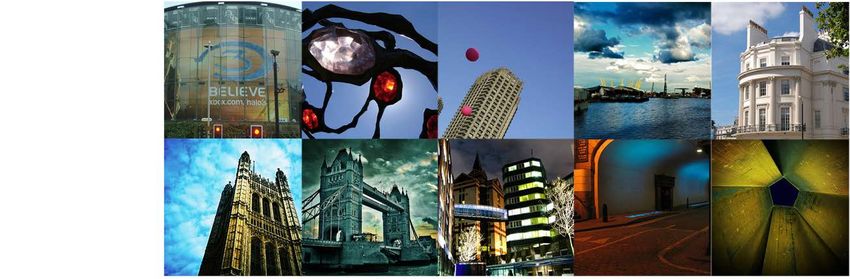
follows: cloudy vs. not-cloudy; hot vs. cold; humid vs. dry;        terms, this intuition translates into saying that i’s distinctive-
high visibility vs. low visibility; windy vs. not-windy.            ness Di is the residual (error) of predicting Ri from Ci . As
                                                                    a proxy for flow Ci , we use the number of distinct subway
                  4    Urban Qualities                              passengers who have visited i.

Before mining those datasets, we need to identify the urban         Subway data. To compute the flow of subway passengers,
qualities that reflect people’s psychological perceptions of        we resort to an anonymized dataset containing a record of
the city.                                                           every journey taken on the London Underground using an
                                                                    Oyster card in the whole month of March 2010. Such cards
4.1   Recognizability                                               are RFID-based technologies that replaced traditional paper-
                                                                    based magnetic stripe tickets in 2003. The dataset contains
Urban sociologists have suggested that the layout of urban
                                                                    76.6 million journeys made by 5.2 million users (each record
spaces affects our sense of community well-being. Everyone
                                                                    consists of a passenger’s trip from station a at time ta , to
living in an urban environment creates their own personal
                                                                    station b at time tb ), and is available upon request from the
“mental map” of the city based on features such as the routes
                                                                    public transportation authority.
they use and the areas they visit. In his 1960 book “The Im-
age of the City”, Kevin Lynch hypothesized that the more
recognizable the features of a city are, the more navigable         Predicting distinctiveness. We have defined distinctiveness
the city is. Good imaginability allows city dwellers to feel at     as the residual (error) of predicting an area’s recognizabil-
home (mental maps of good cities are economical of men-             ity from its number of subway passengers. Thus, to compute
tal effort) and, as a result, their collective well-being thrives   distinctiveness, we need to predict recognizability first and
(Lynch 1960). To put his theory to test, researchers have re-       then quantify the residual of such a prediction. Area i’s pre-
cently used a web game that crowdsources Londoners’ men-            dicted recognizability R̂i is based on the number of unique
tal images of the city (Quercia et al. 2013). The researchers       subway passengers (denoted by Ci ): R̂i = α + βCi 2 . Such
have replicated a well-known pen-and-paper experiment on-           an expression assumes that the flow of subway passengers at
line: that experiment was run in 1972 by Milgram. He re-            a place is a good proxy for the number of people who have
cruited his undergraduates in New York, showed them a vari-         visited the place, which is likely the case in London given
ety of urban scenes, and asked them to guess the locations of       the widespread use of the underground (Smith, Quercia, and
those scenes (Milgram, Kessler, and McKenna 1972). Based            Capra 2013). Upon the predicted values R̂i , we can com-
on the correct answers, he drew the recognizability (collec-        pute the area’s distinctiveness Di , which, given Milgram’s
tive mental) map his students had of New York. The web              original formulation, is the prediction error Di = Ri − R̂i .
game replicates that experiment, in that, it picks up ran-          In words, the less the flow of subway passengers predicts
dom urban scenes and tests users to see if they can judge           recognizability, the more distinctive the area is.
the location in terms of closest subway station, borough, or
region. In analyzing the results, the researchers found that        4.3   Eventfulness
areas suffering from social problems such as housing depri-
vation, poor living conditions, and crime are rarely present        In addition to studying whether an area is simply visited or
in residents’ mental images. We use one of the researchers’         not, one could also consider whether an area is routinely vis-
aggregate datasets. This contains one recognizability score         ited (e.g., the daily street from home to the train station)
for each subway station, and another one for each borough           or whether it is visited in exceptional situations (e.g., dur-
in London. We have 150 tube stations and 30 boroughs be-            ing weekends or holidays). Previous work has partly shown
fore filtering, and 60 stations and 20 boroughs after filtering     that routine places are expected to be associated with geo-
for unreliable scores.                                              referenced content that is less interesting than that associ-
                                                                    ated with places that are visited in exceptional circumstances
4.2   Distinctiveness                                               (Yildirim and Süsstrunk 2013).
                                                                       To capture that intuition, we compute a measure that we
It has been found that people recognize an area because of          call ‘routine score’. We do so on a Foursquare dataset re-
two main reasons: because they are exposed to it (e.g., a cen-      leased by (Cheng et al. 2011): 22,387,930 Foursquare check-
tral area attracts residents from all over the city), and be-       ins collected from September 2010 to January 2011. From
cause the area offers a distinctive architecture (e.g., it hosts    these check-ins, we extracted those that happen to be in Lon-
few star architects’ buildings). In his 1972 article, Milgram       don: 230,785 check-ins in 8,197 places from 8,895 distinct
simplified this idea by introducing the concept of distinc-         users. To avoid computing anomalous scores, we filter out
tiveness. He stated that a place’s recognizability can be ex-       users with less than 10 check-ins and places which were
pressed as Ri = f (Ci · Di ), where f is a function that pre-       visited by less than 10 distinct users. Then, for each user,
dicts a place’s recognizability from the centrality Ci of pop-      we compute the fraction of times (s)he visits each location.
ulation flow (number of people who visit place i) and the           By aggregating those user scores at each location (we used
place’s social or architectural distinctiveness Di . As a result,   a geometric average as scores are skewed), we are able to
an area is socially or architecturally distinctive if its recog-
nizability is not entirely explained by exposure to people but          2
                                                                          The coefficients α and β are those for which the values of Ci
is also partly explained by its distinctiveness. In quantitative    are best predicted from the observed values Ri .
compute a location’s routine score in the range [0, 1]: the of London: darker squares (larger values) contain crowd-
higher it is, the more routine visits the location enjoys. To sourced pictures considered to be beautiful, while lighter
ease illustration, from the routine score, we derive its com- squares (smaller values) contain pictures considered to be
plementary measure, which we call ‘eventfulness score’ and less beautiful. One could then build a predictive model for
is just 1 minus the routine score. beauty that estimates the extent to which those squares
are dark (or light) on input of, say, Flickr or Foursquare
4.4 Beauty, Quiet, and Happiness metadata (e.g., likes on pictures, check-ins in Foursquare
Not only mental maps but also aesthetically pleasing envi- venues). By having this model at hand and stratifying the
ronments are associated with community well-being. Re- input metadata according to, say, time of day (e.g., number
searchers in environmental aesthetics have widely studied of favorites for photos taken at night), one could test which
the relationship between well-being and the ways urban squares the model predicts to be beautiful at night, assuming
dwellers perceive their surroundings (Nasar 1994; Taylor that its predictions do not dramatically change with the con-
2009; Weber, Schnier, and Jacobsen 2008). In 1967, Pe- textual factors. We will test the validity of this assumption
terson proposed a methodology for quantifying people’s in Section 7.
perceptions of a neighborhood’s visual appearance (Peter- The input features are derived from Flickr and
son 1967): he selected ten dimensions that reflected visual Foursquare. These features include number of views, num-
appearance (e.g., preference for the scene, greenery, open ber of favorites, number of comments, number of tags, num-
space, safety, beauty) and had 140 participants rate 23 pic- ber of photos, number of unique Flickr users, number of
tures of urban scenes taken in Chicago along those dimen- unique Foursquare users, and number of check-ins. Since
sions (Peterson 1967). Based on his analysis, he concluded the urban qualities are defined at the levels of subway sta-
that preferences for urban scenes are best captured by asking tion and borough, we aggregate those features at the two lev-
questions concerning the beauty and safety of those scenes: els. Then, if skewed, the features are log-transformed and, as
beauty is synonymous with visual pleasure and appearance. such, their averages are not arithmetic but geometric.
To capture visual pleasure, the concept of beauty is thus key, On input of those features, we put the following models
and that is why it is our first perception quality. Beauty is in- to test: linear model (least squares), decision tree regres-
deed one of the three dimensions that recent work concerned sor, support vector regression, ADA boost regressor, gra-
with urban aesthetics has tried to quantify (Quercia, Ohare, dient boosting regressor, extra trees regressor and random
and Cramer 2013). In this work, researchers collected votes forest regressor. For all the models, we have tried different
on the extent to which hundreds of London urban scenes parameter values and found that the default ones specified
were perceived to be beautiful, quiet, and happy by more in the scikit-learn library4 produced reasonable results. For
than 3.3K crowdsourcing participants. We get hold of the brevity, we report only those results.
scores for beauty, quiet, and happiness at both subway and The predictive accuracies of the models are expressed
borough levels. with two measures: i) Mean Squared Error (MSE), which
The researchers chose quiet because of popular discus- reflects the differences between the values predicted by the
sions on ‘city life’. Sound artist Jason Sweeney proposed model under test and the actual values; and ii) Spearman’s
a platform where people crowdsource and geo-locate quiet rank correlation ρ between two ordered lists of areas: in one
spaces, share them with their social networks, and take au- list, areas are ranked by the model’s predicted values; in the
dio and visual snapshots. It is called Stereopublic3 and is “an other list, areas are ranked by the actual values; ρ ranges
attempt to both promote ‘sonic health’ in our cities and offer from -1 to 1: it is 0 if the two lists are dissimilar, +1 if the
a public guide for those who crave a retreat from crowds” - two lists are exactly the same (best match), and -1 if the two
both for those in need of quietness and for people with dis- lists are exactly reversed.
abilities, like autism and schizophrenia. Figure 3 shows the models’ error values (left panel) and
The remaining quality is that of happiness. This quality accuracy values (right panel) for “in sample” predictions5 .
reflects the ultimate goal behind the 1970s research we have The large pink area reflects the statistical significance of the
referred to: Milgram, Lynch and colleagues were after un- baseline being extremely low. The more sophisticated mod-
derstanding which urban elements help to create intelligible els (e.g., ADA boost, Gradient Boost) perform exceptionally
spaces and would ultimately make residents happy. well, yet simpler models (e.g., linear model, decision tree)
Overall, we consider the three qualities of beauty, quiet, show competitive performance: for all qualities other than
and happiness plus recognizability, distinctiveness, and quiet, the squared errors are below 0.03. The same goes for
eventfulness. Each of those qualities is defined at the two Spearman’s ρ, which is always above 0.50 for all models. If
geographic levels of study: subway and borough levels. we reduce the number of input features from 12 to 6, those
results do not significantly change, suggesting that overfit-
5 Modeling Urban Qualities ting has little to do with such good prediction accuracies. To
To see how our urban qualities change depending on contex- further reinforce this last point, we will now see to which
tual factors, we need to build predictive models for each of extent such predicted values are associated with actual ap-
them. To see why, consider our urban quality of beauty as
4
an example. Its values could be represented on a heat map http://scikit-learn.org/stable/
5
We could not use cross-validation given the limited number of
3
http://www.stereopublic.net/ subway stations or boroughs.Figure 3: Mean Squared Error (left panel) and Spearman’s Correlation ρ (right panel) for Area Rankings Produced by Seven
Models plus Baseline. Each panel shows the results at both borough and subway station levels.
pealing content.
6 Rankings by Urban Qualities
We have just established how accurately off-the-shelf
models can predict the urban qualities from Flickr and
Foursquare metadata. However, we have not yet ascertained
whether the predictions of those models would ultimately re-
sult into the selection of appealing geo-referenced pictures.
To ascertain that, we need to determine which pictures are
to be considered appealing. We do so by resorting to the
widely-used normalized measure of community (user) ap-
peal of picture i (Yildirim and Süsstrunk 2013):
number of favoritesi
appeali =
number of viewsi
Figure 5: Similarity (Spearman’s ρ) between the Ideal List
The higher a picture’s ratio of number of favorites to num-
and a List generated by one of our Urban Qualities. The
ber of views, the more the picture’s views have led to user
similarity between baseline and the ideal list is shown in
likes. Pictures with few views do not need to be filtered away
red with corresponding standard errors. For this barplot, the
as their presence does not affect the overall ranking: pictures
number of pictures per area is set to k = 3.
with many favorites and views will still be highly ranked.
We use the appeal measure to produce lists of geo-
referenced pictures. Each list orders areas in a different way
(we will see how) and, for each area, top k pictures ordered To quantitatively ascertain whether each of those two lists
by appeal are, in turn, shown. Given that pictures are always return appealing content, we build a third one, which we call
ordered by appeal, the desirability of such a list depends on ideal list: in it, pictures are ordered by appeal without any
the ordering of areas. We produce two lists with two distinct consideration for the areas in which they were taken. The
orderings. In the first, areas are ordered at random (baseline more similar the beauty list to the ideal list, the more the
list). In the second list, areas are ordered by a predicted ur- urban quality of beauty is able to promote pictures that users
ban quality (e.g., beauty list) 6 . As a result, both lists contain have liked on Flickr. To measure the similarity of the two
pictures that Flickr users have liked, but the order of areas in lists, we, again, use Spearman’s rank correlation ρ.
one list differs from that in other list. As such, by comparing Figure 5 shows the results, which suggest two notewor-
the two lists, one can establish whether the urban qualities thy considerations. The first is that the baseline list greatly
are useful for ranking city pictures or not. If there is no dif- differs from the ideal list (as the red line shows) and differs
ference between the ways the two lists fare, then either the from the remaining lists related to our urban qualities (sug-
urban quality of, say, beauty does not happen to promote ap- gesting that the ordering of areas matters). The second con-
pealing geo-reference photos or its predicted values do not sideration is that the working hypothesis behind our work
accurately reflect beautiful areas. holds true: ordering areas by a given urban quality tends to
preferentially promote city pictures that are indeed appeal-
6
We use an urban quality’s predicted values and not the actual ing. The quality that most successfully promotes appealing
values to test to which extent our predictions are reasonable and content is that of beauty (ρ = 0.69), followed by recog-
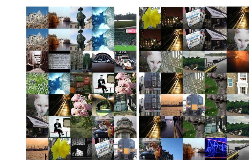
whether they could be used in realistic scenarios. nizability (ρ = 0.58), eventfulness (ρ = 0.53) and distinc-Figure 4: Pictures Ranked by Urban Qualities plus Baseline (last row). As an example, in the first row, top 5 (bottom 5) pictures
in the five most (least), say, recognizable areas are shown.
to be associated with appealing content, while quite areas
are not (the rank by quiet is comparable to the baseline).
This might be because quiet areas either are not associated
with appealing content or are difficult to predict out of the
metadata we have used here. Perhaps, further investigation
should go into enlarging the pool of metadata to include tex-
tual descriptors or even city-wide sound recordings 7 .
7 Contextual Factors
We now study how the predicted values of our urban quali-
Figure 6: Similarity (Spearman’s ρ) between the Ideal List
ties change depending on two contextual variables: time of
and a List Generated by one of our Urban Qualities. The
day, and weather conditions.
similarity varies with the number k of pictures per area (i.e.,
as the recommended list gets longer). To do so, in input of each of the models in the previous
section, we give different features whose values change with
the contextual variables. As we have mentioned in Section 5,
this methodology is valid only if a model does not dramati-
tiveness (ρ = 0.47). These results are further confirmed by
cally change with context. To test this assumption, we study
visually inspecting the set of pictures ranked by each urban
whether the predictive accuracies of our models do not sig-
quality (Figure 4).
nificantly change with time of day or weather, and we find
Figure 6 further shows that the Spearman correlation re- this to be the case (Figure 7).
mains high as the user list of suggested pictures grows: sug-
gesting five or even ten pictures in each area does not de-
7
grade the results at all. We also find that beautiful areas tend http://cs.everyaware.eu/event/widenoiseFigure 7: Accuracy of the Predicted Urban Qualities by Contextual Factors. Similarity (Spearman’s ρ) between predicted and
actual values for different contexts. The correlations do not significantly change for: day vs. night; cold vs. hot; dry vs. humid;
not-cloudy vs. cloudy; low vs. high visibility; not-windy vs. windy.
Figure 8: Rank Correlation (Spearman’s ρ) Between the Figure 11: Pictures in the Top 5 Most Recognizable Areas
Ideal List and a List Generated by one of our Urban Quali- During Hot vs. Cold Days.
ties for Day vs. Night.
Weather Variable Lower Condition Upper Condition
Air temperature cold hot
Wet bulb temp. dry humid
Wind speed not-windy windy
Cloud level not-cloudy cloudy
Visibility low-visibility high-visibility
Figure 9: Pictures in Top 5 most Recognizable Areas at Day Table 1: Binary Discretization of Five Weather Variables.
vs. Night. .
7.1 Time of day weather condition of the day a picture was taken, we asso-
Using the definition of day vs. night in Section 3, Figure ciate the five discretized values with the picture. For exam-
8 shows the similarity (Spearman ρ) between the ideal list ple, for a photo taken at 2007-06-09 17:05, its associated
and a list generated by a given urban quality during different weather variables are: wind speed is 2knots, air tempera-
times of the day. The higher the similarity, the more the gen- ture is 24.7◦ C, wet bulb temperature is 18.0◦ C, cloud level
erated list contains appealing content. We find that beautiful is 6oktas, and visibility is 12km. That translates into as-
areas tend to be associated with appealing content more dur- sociating the following discretized values with the picture:
ing the day than during the night (the cerulean bar decreases hot, humid, not-windy, low-visibility, and not-cloudy. Table
from day to night). In a similar way, eventful areas are as- 3 shows the fraction of photos taken under different weather
sociated with appealing content during the day, which might conditions: as one expects, photos are taken in non-cold and
reasonably suggest that people do not tend explore new parts non-dry days; also, people tend to avoid cloudy days while
of the city at night. Also, by visually inspecting the pictures preferring high visibility days.
in the top 5 most recognizable areas at day vs. those in the Figure 10 shows the similarity (Spearman ρ) between the
top 5 at night (Figure 9), one observes two distinctive sets ideal list and a list generated by a given urban quality under
of results, which speaks to the external validity of our ap- different weather conditions. We find that, with hot weather
proach. (which, in London, means a temperature above 16 degrees
Celsius), any type of area (whether it is recognizable, dis-
7.2 Weather tinctive, eventful, beautiful, or happy) is associated with ap-
For every day present in our weather dataset between 2002 pealing content. Dry and cold turn out to be the weather con-
and 2013, we discretize each of the five weather variables ditions that most negatively affect the production of appeal-
listed in Table 1 into lower class and upper class depending ing content. Again, ranking pictures during hot vs. cold days
on whether their values are in the bottom or upper quartiles results in meaningful and inexpensive segmentations (Figure
(Table 2 shows the resulting thresholds). Depending on the 11).Figure 10: Rank Correlation (Spearman’s ρ) Between the Ideal List and the Lists Generated by one of our Urban Qualities
across Different Weather Conditions.
Weather Condition tlower tupper Units further explore the use of urban features in cold-start situa-
tions, which are increasingly common.
Cold/Hot 7.2 15.9 degC
Dry/Humid 5.8 13.2 degC
Complementary to existing approaches. This work has to
Not-windy/Windy 5.0 11.0 knots
be considered complementary to existing approaches. By
Not-cloudy/Cloudy 2.0 8.0 oktas
no means, it is meant to replace ranking solutions based
Low-visible/High 12.0 29.0 km
on metadata or on visual features. Instead, all these solu-
Table 2: Upper and Lower Thresholds (tlower and tupper ) tions can be used together considering that they work un-
used to Discretize Weather Variables. der different conditions: whenever pictures come with rich
. metadata, then that metadata could be used to rank them;
by contrast, in cold-start situations, our lightweight ranking
combined with visual features might well be the only option
Weather Condition % < tlower % > tupper outside at hand. We have shown that this option is viable as it of-
Cold/Hot 16.4 40.5 43.1 fers good baseline performance. More generally, our results
Dry/Humid 17.5 36.0 46.5 speak to the importance of incorporating cross-disciplinary
Not-windy/Windy 24.2 31.8 44.0 findings. This work heavily borrows from 1970s urban stud-
Not-cloudy/Cloudy 34.4 26.8 38.7 ies and is best placed within an emerging area of Computer
Low-visible/High 18.9 27.3 53.8 Science research, which is often called ‘urban informatics’.
Researchers in this area have been studying large-scale ur-
Table 3: Fraction of Photos Under Different Weather Condi- ban dynamics (Crandall et al. 2009; Cranshaw et al. 2012;
tions. Noulas et al. 2012), and people’s behavior when using
location-based services such as Foursquare (Bentley et al.
2012; Cramer, Rost, and Holmquist 2011; Lindqvist et al.
8 Discussion 2011).
We now discuss the main limitations of this work, and how
to frame it within the context of emerging research. 9 Conclusion
In the web context, the problem of automatic identifica-
Limitations. This work is the first step towards using urban tion of appealing pictures has been often casted as a rank-
features to identify appealing geo-referenced content. In the ing problem. By contrast, in the mobile context, we posited
future, research should go into combining all classes of fea- that the research roadmap should differ and revolve around
tures together. One simple way of doing so is to order each the concept of neighborhood. Before this work, we did not
area’s pictures depending on how appealing they are (ap- know whether and, if so, how some of the 1970s theories
peal can be derived from visual features). The second limi- in urban sociology could be practically used to identify ap-
tation is that new ways of presenting pictures other than seg- pealing city pictures. We have shown that, upon theories
menting them by city neighborhoods (which are politically- proposed by Lynch, Milgram and Peterson, one is indeed
defined and might be arbitrary at times) are in order: one able to do so. We hope that these results will encourage fur-
could, for example, show pictures by areas that emerge from ther work on multi-modal machine learning approaches that
location-based data. Cranshaw et al. (Cranshaw et al. 2012) combine traditional (e.g., visual, textual, and social) features
used Foursquare data to draw dynamic boundaries in the with domain-specific urban features.
city: what they called ‘livehoods’. However, any work that
uses location-based data (including ours) should account for
the limitation of the data itself: the geographic distribution of
References
Foursquare check-ins is biased (Rost et al. 2013) (e.g., a user Bentley, F.; Cramer, H.; Hamilton, W.; and Basapur, S. 2012.
is likely to check-in more at restaurants than at home), and Drawing the city: differing perceptions of the urban environ-
that can greatly affect the computation of our routine scores. ment. In Proceedings of ACM Conference on Human Fac-
Finally, given our promising results, it might be beneficial to tors in Computing Systems (CHI).Cheng, Z.; Caverlee, J.; Lee, K.; and Sui, D. Z. 2011. Ex- Computer Supported Cooperative Work and Social Comput- ploring Millions of Footprints in Location Sharing Services. ing. In ICWSM. Sigurbjörnsson, B., and van Zwol, R. 2008. Flickr Tag Cramer, H.; Rost, M.; and Holmquist, L. E. 2011. Perform- Recommendation Based on Collective Knowledge. In Pro- ing a check-in: emerging practices, norms and ’conflicts’ in ceedings of the 17th ACM Conference on World Wide Web location-sharing using foursquare. In Proceedings of ACM (WWW). International Conference on Human Computer Interaction Smith, C.; Quercia, D.; and Capra, L. 2013. Finger On The with Mobile Devices and Services (MobileHCI). Pulse: Identifying Deprivation Using Transit Flow Analy- Crandall, D. J.; Backstrom, L.; Huttenlocher, D.; and Klein- sis. In Proceedings of ACM International Conference on berg, J. 2009. Mapping the world’s photos. In Proceed- Computer-Supported Cooperative Work (CSCW) . ings of ACM International Conference on World Wide Web Taylor, N. 2009. Legibility and aesthetics in urban design. (WWW) . Journal of Urban Design 14(2):189–202. Cranshaw, J.; Schwartz, R.; Hong, J.; and Sadeh, N. 2012. van de Sande, K. E.; Gevers, T.; and Snoek, C. G. 2011. The Livehoods Project: Utilizing Social Media to Under- Empowering Visual Categorization With the GPU. IEEE stand the Dynamics of a City. In International AAAI Con- Transactions on Multimedia 13(1). ference on Weblogs and Social Media (ICWSM). van Zwol, R.; Rae, A.; and Garcia Pueyo, L. 2010. Predic- Datta, R.; Joshi, D.; Li, J.; and Wang, J. Z. 2006. Studying tion of Favourite Photos Using Social, Visual, and Textual Aesthetics in Photographic Images Using a Computational Signals. In Proceedings of ACM Conference on Multimedia Approach. In Proceedings of the 9th European Conference (MM) . on Computer Vision (ECCV). Weber, R.; Schnier, J.; and Jacobsen, T. 2008. Aesthetics Lindqvist, J.; Cranshaw, J.; Wiese, J.; Hong, J.; and Zim- of streetscapes: Influence of fundamental properties on aes- merman, J. 2011. I’m the mayor of my house: examining thetic judgments of urban space 1, 2. Perceptual and motor why people use foursquare - a social-driven location sharing skills 106(1):128–146. application. In Proceedings of ACM Conference on Human Yildirim, G., and Süsstrunk, S. 2013. Rare is Interesting: Factors in Computing Systems (CHI). Connecting Spatio-temporal Behavior Patterns with Subjec- Lynch, K. 1960. The Image of the City. Urban Studies. MIT tive Image Appeal. In Proceedings of the 2nd ACM Inter- Press. national Workshop on Geotagging and Its Applications in Martı́nez, P., and Santamarı́a, M. 2012. Atnight: Visions Multimedia (GeoMM). through data. Mass Context 172–183. Milgram, S.; Kessler, S.; and McKenna, W. 1972. A Psy- chological Map of New York City. American Scientist. Nasar, J. L. 1994. Urban design aesthetics: The evaluative qualities of building exteriors. Environment and Behavior 26(3):377. Noulas, A.; Scellato, S.; Lambiotte, R.; Pontil, M.; and Mas- colo, C. 2012. A Tale of Many Cities: Universal Patterns in Human Urban Mobility. PLoS ONE. Peterson, G. L. 1967. A Model of Preference: Quantita- tive Analysis of the Perception of the Visual Appearance of Residential Neighborhoods. Journal of Regional Science 7(1):19–31. Quercia, D.; Pesce, J. P.; Almeida, V.; and Crowcroft, J. 2013. Psychological Maps 2.0: A web gamification enter- prise starting in London. In Proceedings of ACM Interna- tional Conference on World Wide Web (WWW) . Quercia, D.; Ohare, N.; and Cramer, H. 2013. Aesthetic Capital: What Makes London Look Beautiful, Quiet, and Happy? Redi, M., and Merialdo, B. 2012. Where is the Beauty?: Re- trieving Appealing Video Scenes by Learning Flickr-based Graded Judgments. In Proceedings of the 20th ACM Con- ference on Multimedia (MM). Rost, M.; Barkhuus, L.; Cramer, H.; and Brown, B. 2013. Representation and communication: Challenges in interpret- ing large social media datasets. In 16th ACM Conference on
You can also read