Assessment of the Performance of Satellite-Based Precipitation Products for Flood Events across Diverse Spatial Scales Using GSSHA Modeling System ...
←
→
Page content transcription
If your browser does not render page correctly, please read the page content below
geosciences
Article
Assessment of the Performance of Satellite-Based
Precipitation Products for Flood Events across Diverse
Spatial Scales Using GSSHA Modeling System
Chad Furl, Dawit Ghebreyesus and Hatim O. Sharif *
 Department of Civil and Environmental Engineering, University of Texas at San Antonio, 1 UTSA Circle,
 San Antonio, TX 78249, USA; chad.furl@gmail.com (C.F.); dawit.ghebreyesus@my.utsa.edu (D.G.)
 * Correspondence: hatim.sharif@utsa.edu; Tel.: +1-210-458-6478

 Received: 21 April 2018; Accepted: 24 May 2018; Published: 28 May 2018

 Abstract: Accurate precipitation measurements for high magnitude rainfall events are of great
 importance in hydrometeorology and climatology research. The focus of the study is to assess the
 performance of satellite-based precipitation products against a gauge adjusted Next-Generation Radar
 (NEXRAD) Stage IV product during high magnitude rainfall events. The assessment was categorized
 across three spatial scales using watershed ranging from ~200–10,000 km2 . The propagation of the
 errors from rainfall estimates to runoff estimates was analyzed by forcing a hydrologic-model with the
 satellite-based precipitation products for nine storm events from 2004 to 2015. The National Oceanic
 and Atmospheric Administration (NOAA) Climate Prediction Center (CPC) Morphing Technique
 (CMORPH) products showed high correlation to the NEXRAD estimates in all spatial domains, and
 had an average Nash-Sutcliffe coefficient of 0.81. The Global Precipitation Measurement (GPM) Early
 product was inconsistent with a very high variance of Nash-Sutcliffe coefficient in all spatial domains
 (from −0.46 to 0.38), however, the variance decreased as the watershed size increased. Surprisingly,
 Tropical Rainfall Measuring Mission (TRMM) also showed a very high variance in all the performance
 statics. In contrast, the un-corrected product of the TRMM showed a relatively better performance.
 The errors of the precipitation estimates were amplified in the simulated hydrographs. Even though
 the products provide evenly distributed near-global spatiotemporal estimates, they significantly
 underestimate strong storm events in all spatial scales.

 Keywords: hydrology; NEXRAD; remote sensing; GSSHA; flooding; GPM

1. Introduction
      Accurate precipitation measurements for high magnitude events are of key importance to a
number of areas in hydrometeorology and climatology research. In addition to research pursuits, these
measurements have great value to public well-being by providing the backbone of rainfall-runoff
prediction systems aimed at forecasting floods [1,2]. Over the past couple of decades in operational
settings, these datasets have primarily been generated with radar and rain gauge networks [3]. Radar
networks have the advantage of providing near real-time information over a continuous region at very
fine scales, mostly unattainable with ground-based gauge networks. Numerous validation studies
showed good performance of radar measurements, especially when combined with gauge networks for
bias adjustments/quality control (e.g., Wang, Xie [4], Habib, Larson [5]). However, lack of even global
distribution of radar network and problems such as beam blockage in complex terrain introduced
significant gaps in radar coverage that pushed researchers to explore robust solution [6].
      Satellite precipitation estimates provide a means for timely, near-global precipitation estimates,
and much of the recent effort has been put into their validation and verification [7–13]. Several

Geosciences 2018, 8, 191; doi:10.3390/geosciences8060191                   www.mdpi.com/journal/geosciences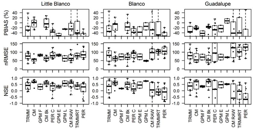
Geosciences 2018, 8, 191                                                                            2 of 18

products, including those provided by the recently launched Global Precipitation Measurement (GPM)
mission, now provide the spatiotemporal resolution needed to forecast or conduct post-event analysis
of flash floods. Even though the potential of satellite-based products was highly regarded, their
poor performances were reported widely across the globe, especially, in their ability to accurately
capture high magnitude precipitation events. Nikolopoulos, Anagnostou [14] demonstrated mean areal
precipitation is consistently underestimated in their satellite ensemble analysis of a high magnitude
precipitation event in Italy. AghaKouchak, Behrangi [15] examined several operational satellite
precipitation products across the southern Great Plains with respect to precipitation thresholds and
demonstrated the detection skill reduces as the choice of extreme threshold decreases. Mehran and
AghaKouchak [16] reported similar findings when comparing three operational satellite products
across the conterminous United States. Mei, Anagnostou [17] showed that satellite precipitation
estimates are more biased for frontal events than for short-duration events. However, the error
statistics of the products showed higher variability for the latter. Moreover, the products showed high
inconsistency across different terrain [12] and climatic conditions [11]. These and other studies stress
the need for more analysis and evaluation of the accuracy and performance of recent satellite products
in capturing the behavior of extreme precipitation events by comparing them against products from
ground-based measurement networks (radar or rain gauges).
      Satellite-based precipitation products were found to be more accurate in a dry season and
in wet tropical and dry zones than in semi-arid and mountainous regions. The uncertainty
amongst the products was higher in estimating heavy rainfall storms in a semi-arid area. Moreover,
the products, in general, overestimate the number of rainy days and underestimate the heavy
rainfall storms [11]. Amongst the highly cited satellite-based products in the literature, the National
Oceanic and Atmospheric Administration (NOAA) Climate Prediction Center (CPC) Morphing
Technique (CMORPH) and Precipitation Estimation from Remotely Sensed Information using Artificial
Neural Networks (PERSIANN)were reported to be spatially inconsistent [10–12,18–20]. The Tropical
Rainfall Measuring Mission (TRMM) and its continuation mission GPM were found in many studies
to be relatively consistent and more accurate but overestimated the average rainfall events and
underestimated the heavy storm events in general [11–13,19,21].
      The potential of high-resolution satellite precipitation estimates in hydrological applications
is supported by the facts that satellite measurements are not inhibited by local topography and
are available at a global scale. Forcing hydrological models with high-resolution satellite-based
precipitation products can provide a streamflow forecast for ungauged, complex terrain basins. The
manner in which rainfall errors propagate through a hydrologic model has important implications for
building operational flow forecasts for such basins. Propagation of errors is influenced by spatial and
temporal resolution of the satellite estimate, basin scale, and complexity of the physical interactions
represented by the watershed model, among others. Presently, the majority of detailed error
propagation studies were forced with radar rainfall data (e.g., Sharif, Ogden [22], Sharif, Ogden [23,24],
Vivoni, Entekhabi [25]) with comparatively less work done for satellite-based precipitation (e.g.,
Nikolopoulos, Anagnostou [14], Gebregiorgis, Tian [26], Maggioni, Vergara [27], Chintalapudi,
Sharif [28]). Moreover, most of the studies forced by satellite-based precipitation on propagation
error into hydrologic predictions were focused on grid-based evaluation or long-term basin-averaged
runoff response (e.g., Su, Gao [29], Wu, Adler [30]).
      Spatial scale (with respect to both satellite resolution and basin size) is an important aspect
in rainfall-to-runoff error propagation for satellite precipitation, and a more comprehensive
understanding of it plays a vital role in mitigation of natural disasters. Nikolopoulos, Anagnostou [14]
developed satellite rainfall ensembles for a single flood event and showed error propagation is
strongly related to the size and characteristics of the watershed and the satellite product resolution.
A rainfall-runoff process reduces the satellite-precipitation error variance in a mild-sloped catchment,
and this effect exhibits the basin-scale dependence [31]. However, many other factors also have a
Geosciences 2018, 8, 191                                                                            3 of 18

significant impact, such as precipitation type, magnitude, and spatiotemporal pattern, and basin
characteristics interact with the scale effect [31–33].
      The Gridded Surface Subsurface Hydrologic Analysis (GSSHA) model, which is fully distributed
and physically-based, was developed by the Department of Defense in order to simulate surface flows
in non-Hortonian watersheds and watersheds with diverse characteristics of runoff production [34].
The model employs a mass-conserving solution of partial differential equations to produce the different
components of hydrologic processes. The model was able to reproduce stream flows from a very
diverse watershed with reasonable accuracy [35]. Moreover, the grid size can be used to optimize the
required accuracy with the required computational power [36].
      In the present study, the performance of several satellite precipitation products with respect to
gauge corrected ground-based radar estimations for nine moderate to high magnitude events across
the Guadalupe River system in south Texas was investigated. The analysis was conducted across
three nested watersheds (ranging from 200 to 10,000 km2 in area) to capture and quantify the effect
of the scale on the propagation of the error. Satellite-based precipitation data sets were used to force
a fully distributed physics-based Gridded Surface Subsurface Hydrologic Analysis (GSSHA) model
to examine error propagation through the hydrologic model. Both gauge-corrected and uncorrected
satellite products were used, encompassing a variety of latency times, spatial resolutions, and temporal
resolutions. Satellite-based precipitation datasets used in the study include various products from
GPM, PERSIANN system, CMORPH, and TRMM.

2. Materials and Method

2.1. Watershed
     The Guadalupe River originates in south-central Texas and flows southeasterly until emptying
into the Guadalupe estuary/Gulf of Mexico. In this study, the testbed is the middle and upper
portions of the basin, with the watershed outlet taken near Gonzales, TX past the confluence of the
Guadalupe and San Marcos rivers (herein referred to as Guadalupe basin). At the outlet, the basin
drains approximately 9000 km2 . Two additional catchments within the watershed were delineated for
scale effect analysis: Little Blanco River (178 km2 ) and the Blanco River (1130 km2 ). The spatial extent
of the Guadalupe watershed along with the two nested watersheds is shown in Figure 1. Canyon Lake
reservoir is formed by an impoundment along the Guadalupe River and contains significant flood
storage, thus, we removed the dam from our watershed model to simulate a naturally flowing river
for the analysis of hydrograph error propagation.
     The Guadalupe River flows across distinct landscapes with varying hydrological characteristics.
The upper portion of the watershed is located in an area known as the Texas Hill Country. This region
is comprised of a karstic landscape with steep surfaces, exposed bedrock, and very thin clayey soils.
As the river passes through the Balcones Escarpment, it encounters the Edwards Aquifer recharge
and artesian zones. In these regions, soils are permeable and there is much groundwater-surface
water interaction. The lower portion of the river crosses the Blackland Prairies before entering the
Coastal Plain. A generalized soil map of the study area including the recharge and artesian areas of
the Edwards Aquifer is displayed in Figure 1. There are a number of studies available describing the
surface characteristics of the watershed in detail along with its flood hydrology [36–38].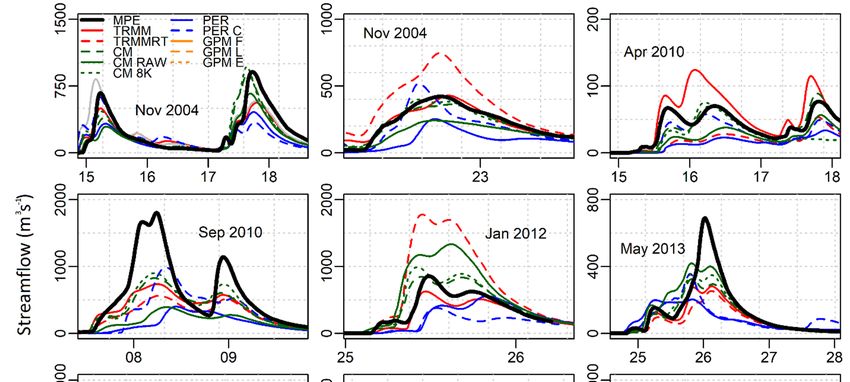
drains approximately 9000 km2. Two additional catchments within the watershed were delineated
for scale effect analysis: Little Blanco River (178 km2) and the Blanco River (1130 km2). The spatial
extent of the Guadalupe watershed along with the two nested watersheds is shown in Figure 1.
Canyon Lake reservoir is formed by an impoundment along the Guadalupe River and contains
significant   flood
Geosciences 2018, 8, 191storage, thus, we removed the dam from our watershed model to simulate       a
                                                                                                4 of 18
naturally flowing river for the analysis of hydrograph error propagation.

                                                 N

    Figure
    Figure 1.
            1. Location
                Locationand
                         andarea
                             areamap
                                  mapofofthe
                                          thestudy
                                               studywatersheds
                                                     watershedsalong with
                                                                 along    a generalized
                                                                       with             soil
                                                                            a generalized    map.
                                                                                          soil    Each
                                                                                               map.    of
                                                                                                    Each
    the three interior watersheds are outlined,  and the Edwards  Aquifer recharge and artesian zones
    of the three interior watersheds are outlined, and the Edwards Aquifer recharge and artesian zonesare
    displayed.
    are displayed.

2.2. Storm Events
      The Texas Hill Country is one of the most flash flood-prone areas of the entire United States due
to its flood-prone physiography and susceptibility to extreme precipitation [38,39]. Although not
considered among the very humid regions of the U.S., proximity to the Gulf of Mexico allows for
extremely moist tropical air masses to reach the Balcones Escarpment where they can be subjected to
orographic lift [40]. The region holds or has held several precipitation world records on time scales less
than 24 h (USGS 2014). The precipitation envelope curve for Texas is comprised mostly from events in
this region with others from the coastal plain. Once precipitation falls, the availability of steep slopes,
high drainage density, exposed bedrock, and clay-rich soils have the ability to produce extremely high
runoff coefficients with short lag times [41].
      Here, nine large precipitation events from 2004–2015 across the middle Guadalupe basin
were selected to examine satellite precipitation estimate performance and hydrologic model error
propagation. All of the storm event accumulations from the Stage IV precipitation record are presented
in Figure 2. The hydrometeorology of several of these events has been examined in detail including
Furl, Sharif [42] (May 2015 event), Furl, Sharif [40] (September 2010 event), and Sharif, Sparks [36]
(November 2004 events).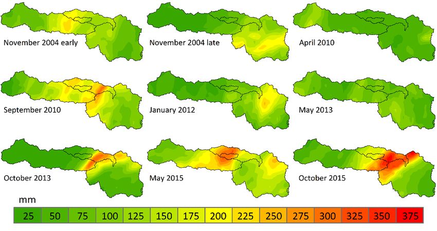
Here, nine large precipitation events from 2004–2015 across the middle Guadalupe basin were
selected to examine satellite precipitation estimate performance and hydrologic model error
propagation. All of the storm event accumulations from the Stage IV precipitation record are
presented in Figure 2. The hydrometeorology of several of these events has been examined in detail
including2018,
Geosciences Furl,  Sharif [42] (May 2015 event), Furl, Sharif [40] (September 2010 event), and Sharif,
               8, 191                                                                           5 of 18
Sparks [36] (November 2004 events).

     Figure 2. Total accumulations from stage IV data for individual storm events used in the analysis
     Figure 2.
     (mm). The  month and
     (mm). The month       year in
                       and year in which
                                   which the
                                          the storm
                                              storm occurred
                                                    occurred is
                                                             is displayed
                                                                displayed along
                                                                          along with
                                                                                 with outlines
                                                                                      outlines of
                                                                                               of the
                                                                                                  the interior
                                                                                                      interior
     watersheds.
     watersheds. Numbers
                 Numbers along
                           along the
                                  the legend
                                      legend represent
                                              represent the
                                                        the maximum
                                                            maximum value
                                                                       value from
                                                                              from each
                                                                                   each category.
                                                                                        category.

2.3. Precipitation Datasets
     In total, ten satellite precipitation products were examined,
                                                           examined, encompassing a variety of
spatiotemporalresolutions.
spatiotemporal   resolutions. Moreover,
                            Moreover,      the examined
                                      the examined        products
                                                   products          include
                                                            include gauge     gauge and
                                                                           corrected   corrected and
                                                                                          uncorrected
products to assess the impact of the adjustment. A brief description of the precipitation products is
included below.

2.3.1. NEXRAD Stage IV
     Each of the satellite precipitation datasets was compared to the National Weather Service (NWS)
and the National Centers for Environmental Prediction (NCEP) stage IV Quantitative Precipitation
Estimate (herein Stage IV) [43]. The precipitation estimate is a quality controlled multi-sensor product
(radar and gauges) produced by NCEP from the NEXRAD Precipitation Processing System [44] and the
NWS River Forecast Center precipitation processing [45]. Precipitation bins are 4 km × 4 km and have
an hourly temporal resolution. The primary radar operating across the study area is National Weather
Service in Austin/San Antonio (KEWX) station approximately 70 km from the watershed outlet.
     The authors acknowledge the inherent biases that accompany radar-based precipitation estimates.
However, the relatively fine space-time scales of the dataset provide the best means to describe
the spatiotemporal heterogeneity of the rainfall across the basin and make satellite comparisons.
Moreover, previous studies by the authors demonstrated that Stage IV products were more suitable
than observations by typical rain gauge networks as inputs to physically based distributed-parameter
models (e.g., [28,36]).

2.3.2. GPM
     The GPM core observatory was launched on 27 February 2014 providing a new means of satellite
global precipitation measurement. The GPM consists of a core-satellite and numerous others in its
constellation. The GPM mission is based on a constellation of microwave radiometers and integrated
IR sensors to cover the blind spot of the microwave sensors. The Integrated Multi-Satellite Retrievals
for GPM (IMERG) is the precipitation product developed by the GPM network. The core GPM
satellite carries a dual-frequency precipitation radar along with multichannel microwave imagers and
is used for calibration of the constellation satellites. Additionally, GPM can integrate infrared (IR)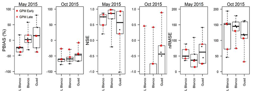
Geosciences 2018, 8, 191                                                                            6 of 18

measurements from geostationary data to cover areas not seen by constellation satellites. The data
produces a near global precipitation product with a spatial resolution of 0.1◦ and 30-min temporal
resolution [46,47].
     IMERG output is available in Early, Late, and Final runs, with a latency of approximately 4 h,
18 h, and 4 months, respectively. The Final IMERG run is calibrated by monthly gauge precipitation
data following a certain procedure (Huffman, Bolvin [46]). In the present study, version 3 processing
algorithms were used, and each of the three IMERG products were examined.

2.3.3. PERSIANN
     The PERSIANN system estimates rainfall from infrared image data provided by geostationary
satellites. PERSIANN data are calibrated in real time from independent microwave precipitation
estimates. The calibration process is based on an adaptive training technique which updates neural
network parameters when microwave data are available [48]. The data are available in 0.25◦ , 30-min
resolution approximately 2 days after the gridded IR images are collected. The rainfall product covers
tropical and middle latitudes from 50 S to 50 N [48,49].
     PERSIANN-Cloud Classification System (PERSIANN-CCS) allows for precipitation estimates at
the same temporal resolution and a finer spatial resolution (0.04◦ ). Additionally, the data are available
in near real-time. The system allows for the discernment and classification of cloud patch features
based on height, areal extent, and variable texture. These classifications are used to further refine
the assignment rainfall within each cloud. The product with a latency of two days was used for
PERSIANN-CCS in this study.

2.3.4. CMORPH
     CMORPH estimates precipitation from microwave-based precipitation images advected in time
using infrared images from geosynchronous satellites. The product combines the positive side of
the two satellites: estimated precipitation from low orbited satellites using microwave images and
transportation of the estimated precipitation in time using the IR from the geosynchronous satellites.
Microwave images are much better in estimating precipitation but they are not continuous, and IR
from geosynchronous satellites are available and are continuous in time. The precipitation product
is available at 30 min intervals with 8 km resolution as well as 3-h, 0.25◦ resolution. Precipitation
estimates are available approximately 18 h past instrument measurement [50]. CMORPH products used
in this study include the raw satellite-only precipitation product (CMORPH_RAW), the climate data
record (CDR) version (CMORPH CDR) and the published 8 KM resolution product CMORPH 8KM.

2.3.5. TRMM
     The Tropical Rainfall Measuring Mission (TRMM) employs a combination of microwave and
IR data to estimate precipitation at 0.25◦ every 3 h. The TRMM product is produced by combining
microwave estimates which are used to calibrate IR estimates from geosynchronous satellites. The IR
estimates are used to fill gaps left by the microwave sensors. TRMM 3B42 V7 and TRMM-RT 3B42
V7 were used in the study. Gridded monthly rain gauge values are used to adjust the TRMM 3B42
V7 estimates [51]. The TRMM-RT (Real-Time) product is a near real-time dataset with no gauge
adjustments. An overview of the availability of the entire dataset is shown in Table 1.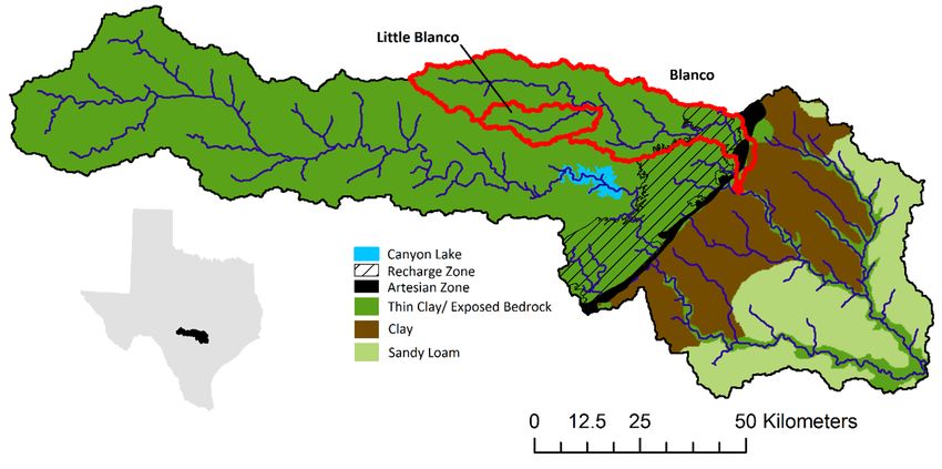
Geosciences 2018, 8, 191                                                                                          7 of 18

                           Table 1. Description of satellite precipitation dataset availability.

                           Nov. 2004     Nov.      Apr.   Sept.    Jan.     May      Oct.    May    Oct.    Gauge
                            Early      2004 Late   2010   2010     2012     2013     2013    2015   2015   Adjusted
       TRMM B42               x           x         x       x        x       x        x        x     x        Y
      TRMM-RT B42             x           x         x       x        x       x        x        x     x        N
       PERSIANN               x           x         x       x        x       x        x        x     x        N
     PERSIANN CCS             x           x         x       x        x       x        x        x     x        N
      CMORPH CDR              x           x         x       x        x       x        x       NA    NA        Y
      CMORPH 8KM              x           x         x       x        x       x        x       NA    NA        Y
      CMORPH RAW              x           x         x       x        x       x        x        x     x        N
    GPM IMERG EARLY          NA          NA        NA      NA       NA      NA       NA        x     x        N
    GPM IMERG LATE           NA          NA        NA      NA       NA      NA       NA        x     x        N
    GPM IMERG FINAL          NA          NA        NA      NA       NA      NA       NA        x     x        Y

2.4. Hydrologic Model
      Precipitation datasets were used to force the fully distributed physics-based GSSHA model [34,52].
Hydrological processes simulated included infiltration, landscape retention, overland flow, and stream
routing. Evapotranspiration and deep aquifer contributions were assumed to be insignificant relative
to the processes since the simulation is event based. Model preprocessing was conducted using ArcGIS
and Aquaveo’s Watershed Modeling System. Watershed terrain was constructed from USGS 10 m
digital elevation models (DEM) filled using the Cleandam algorithm distributed with the GSSHA
model. Land use and land cover data were extracted from the National Land Cover Database 2011
(NLCD 2011) dataset. Soils data were prepared from SSURGO datasets along with maps from the
Edwards Aquifer Authority defining the Edwards Aquifer recharge zone.
      Infiltration calculations were conducted using Green and Ampt with redistribution [53] and
pre-calibrated saturated hydraulic conductivity values taken from Rawls, Brakensiek [54]. Grid cells
were assigned to one of four land use classes for retention and overland roughness. Stream channels
were modeled using irregular cross sections for the main channel and large tributaries. The irregular
channel and floodplain geometry were extracted from a triangular irregular network constructed from
the DEM allowing for control of floodplain simulation. Upland tributaries were modeled as a uniform
trapezoidal profile. Reach specific Manning’s n values were assigned based on field observations and
prior modeling experience in this region of Texas. Routing was calculated using the diffusive wave
equation in 1D for streams and 2D for overland flow. The hydrological model was run on a 150-m grid
cell size with a 1-min simulation time step.
      Distributed models have the distinct advantage of allowing examination of hydrologic properties
at any point in the basin. In this study, three watershed models were constructed: Blanco watershed,
Upper Guadalupe watershed, and Middle Guadalupe watershed. Results from the Little Blanco
watershed were harvested from the proper interior node of the Blanco River watershed model.
The Middle Guadalupe model (i.e., implementation of the hydrologic model over Middle Guadalupe)
used streamflow from the outlets of the Blanco and Upper Guadalupe as boundary condition inflows,
thereby allowing a very fine gridded distributed model over a 9000 km2 basin. The Upper Guadalupe
model discharge hydrograph was input into the Middle Guadalupe at the outlet of Canyon Lake,
bypassing the reservoir.
      The Blanco watershed model was the primary model calibrated. Furl et al. [42] calibrated the
model to the November 2004 “early” event used here and achieved r2, Nash-Sutcliffe model efficiency
(NSE), and percent bias (PBIAS) values of 0.91, 0.90, and 10.2%, respectively for the calibration run.
Similar model parameter values were used for the Upper Guadalupe model. The setup for the Middle
Guadalupe followed hydrologic parameters described by Sharif, Sparks [36], which described the
November 2004 “late” event. It should be noted that our main objective with model calibration is to
provide realistic rainfall-runoff mechanisms such that error propagation analysis can be conducted.
Surface properties for the Blanco River watershed are shown in Table 2. The readers are directed to
Sharif, Sparks [36] and Furl et al. [42] for detailed descriptions of the watershed models and their
comparisons with measured flows.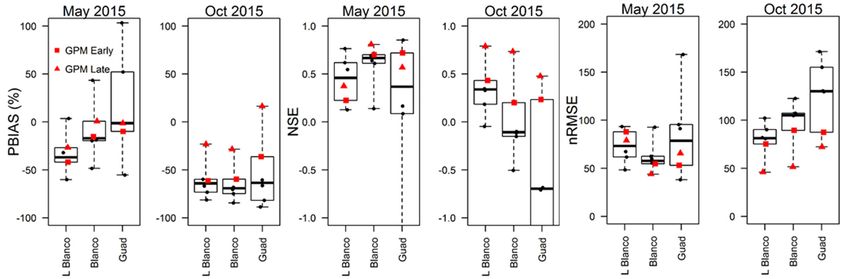
Geosciences 2018, 8, 191                                                                                 8 of 18

      Table 2. Gridded Surface Subsurface Hydrologic Analysis (GSSHA) infiltration and overland flow
      parameters for the Blanco watershed model.

                           Saturated Hydraulic                                    Manning’s
      Soil Texture/                               Capillary           Effective                  Retention
                              Conductivity                                         Roughed
       Land Use                                   Head (cm)           Porosity                  Depth (mm)
                                (cm·hr−1 )                                        Coefficient
     Recharge zone                10.0               23.6               0.417          -            -
          Clay                     1.2               0.06               0.385          -            -
         Loam                     0.01                1.3               0.434          -            -
       Fine loam                  0.02               2.18               0.412          -            -
        Fine silt                 0.01               0.68               0.486          -            -
       Fine sand                  0.03               23.6               0.417          -            -
         Urban                      -                  -                  -          0.18          5.0
         Forest                     -                  -                  -          0.25          5.0
         Shrub                      -                  -                  -          0.20          5.0
    Grasslan/agriculture            -                  -                  -          0.30          5.0

2.5. Evaluation Criteria
      Satellite precipitation results were analyzed by comparing mean areal precipitation hyetographs
with those generated from the Stage IV precipitation record. Here, the reference hydrographs were
those driven by the reference precipitation product (radar). It will not be appropriate to use observed
hydrographs as a reference since we do not have a precipitation product that will perfectly produce the
observed hydrographs. A weighting method was used in the averaging routine to account for rainfall
bins only partially covering a portion of the basin. For comparisons, satellite hyetographs were scaled
to a one-hour time step using a simple linear transformation in order to match the Stage IV record.
The comparison period was confined to when the Stage IV record indicated 1 mm of precipitation had
fallen across the basin until rainfall ceased. Streamflow hydrograph comparisons were conducted in a
similar manner by comparing satellite generated model output with the hydrograph generated by the
Stage IV record. The analysis period was determined by visually examining the Stage IV generated
hydrographs and capturing from just before the rising limb of the hydrograph until after the falling
limb. The comparisons for hyetographs and hydrographs were completed using the percent bias
(PBIAS), normalized root-mean-square-error (nRMSE), and Nash-Sutcliffe model efficiency (NSE)
statistics. Simple relative error in precipitation, peak flow, and volume of flow was calculated for
error propagation analysis. Calculations were completed using the hydroGOF package [55] in R
environment as follows:
                                                       ∑ N ( S i − Oi )
                                       PBIAS = 100 × i=1 N                                           (1)
                                                            ∑ i = 1 Oi
                                                     q
                                                        1    N                 2
                                                        N ∑ i = 1 ( S i − Oi )
                                   nRMSE = 100 ×                                                     (2)
                                                               nval
                                          (
                                                    sd(Oi ), norm = “sd”
                            where nval =
                                             Omax − Omin , norm = “maxmin”
                                                                            2
                                                             ∑iN=1 (Si − Oi )
                                             NSE = 1 −                      2                               (3)
                                                             ∑iN=1 Oi − O
                                                             ∆x  x −x  x
                                    relative error (δx ) =      = 0   = 0 −1                                 (4)
                                                              x     x   x
where:

Si is the simulated rainfall (estimated by the product),
Oi is the estimated rainfall by NEXRAD stage IV,
x0 is the estimated rainfall by the product/precipitation/simulated peak flow with the product, and
x is the estimated rainfall NEXRAD stage IV/simulated peak flow with NEXRAD stage IV rainfall.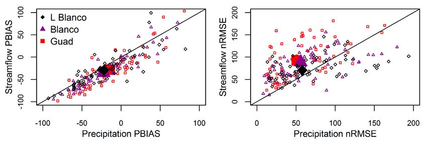
Geosciences 2018, 8, 191 9 of 18
Geosciences 2018, 8, x FOR PEER REVIEW 9 of 17
3. Results and Discussion
Generally, the satellite-based precipitation products showed less variability in the case of the
3.1. Precipitation
Guadalupe basin (Large) relative to the two smaller watersheds (Figure 4). This could be mainly
Precipitation
because from thepower
of the smoothing StageofIVmean record averaged
value over theover largethe entiredomain
spatial watershed ranged
(filtering from
the noise
approximately
introduced by the products). Both products from CMOPRH (labeled as CM and CM 8K) showed 72
50–150 mm, and storm durations lasted from just a few hours to approximately h.
very
Among the 27 isolated storm event and watershed size combinations (9 storm
high correlation with the stage IV product in all spatial domains with very high Nash coefficient. events × 3 watersheds),
the
GPM satellite-based
Early was foundprecipitation products showed
to be inconsistent with a very a widehighrange
variancelevelofofNash
accuracy when compared
coefficient to
in all spatial
the Stage IV estimates. As shown in Figure 3, for the largest spatial
domains, however, the variance was decreased as the watershed size increase. Surprisingly, TRMM domain, satellite precipitation
estimates
showed ashowed
very highthevariance
ability toin very
all closely match radar
the performance results
statics, (November
especially 2004two
in the (late),
smallMay 2013), and
watersheds.
consistently overestimate (November 2004, early) and also systematically
In contrast, the TRMM-RT product showed relatively better performance. As described above, the underestimate precipitation
(October
performance 2015). The products
of GPM Final producttendedwas to significantly
inferior to the underestimate
earlier ones. The in four events
whole and onlyofonce
distribution the
overestimated when compared to NEXRAD
performance statistics is provided in Figure 4. Stage IV estimates. In addition to the inherent errors
in theInsatellite
order toproducts
provide due
some tocomparison
calibration and the rainfall
between estimation
satellites products,technique
performance (i.e.,statistic
microwave or
results
infrared), the relatively coarse resolution of the products may have contributed
were pooled from all spatial domains for each individual satellite product. Table 3 displays the to the underestimations
errors.
median,Underestimation
average, and range is of
more pronounced
the statistics afterfor
thisthe large events
aggregation. Forwhere
the 0.25°satellite underestimates
uncorrected products,
the high intensity periods. Interestingly, the Final GPM
performance statistics indicated CMORPH RAW > TRMM-RT > PERSIANN for the nine product underestimates rainfall more than
events
the earlier products.
examined. Sapiano and This can also
Arkin [10] be attributed
found to the nature
that correlations were ofhighest
the eventswithwhere
CMORPH climatology and
in an inter-
gauge adjustments did not capture the localized intensity of the events.
comparison and validation study on sub-daily satellite precipitation data. For the gauge corrected In the rest of the four storm
events,
products theatNEXRAD product
0.25°, there was very seemedlittletodifference
fit the averagebetween of allTRMM
the satellite-based
and CMORPH products
when(Figure
the same3).
The satellite-based
events were compared products
(2015failed
events to unavailable
capture the storm events that
for CMORPH). It occurred
is difficultintothedraw
Fall (September,
conclusions
October)
about the performance of GPM given that only two events were measured. GPM results areIn
with the exception of the 2004 storm where they tended to overestimate the storm. contrast,
compared
the margin of error was very low in storm
to the other products for the 2015 events below. events that occurred in May.
Figure 3. Storm
Stormevent
eventrainfall
rainfallaccumulations
accumulationsaveraged
averagedover
overthethe
Blanco watershed.
Blanco Legend
watershed. labels
Legend are
labels
abbreviated
are as follows:
abbreviated MPE—Stage
as follows: IV, TRMM—TRMM
MPE—Stage IV, TRMM—TRMM 3B42, CM—CMORPH CDR, GPM
3B42, CM—CMORPH CDR,F—GPM
GPM
IMERG FINAL,
F—GPM IMERGCM 8K—CMORPH
FINAL, 8KM, PER
CM 8K—CMORPH C—PERSIANN
8KM, CCS, GPM
PER C—PERSIANN E—GPM
CCS, IMERG EARLY,
GPM E—GPM IMERG
EARLY, GPM L—GPM
GPM L—GPM IMERG
IMERG LATE, CMLATE, CM RAW—CMORPH
RAW—CMORPH RAW, TRMM-RT—TRMM-RT
RAW, TRMM-RT—TRMM-RT 3B42,
3B42, and PER—
and PER—PERSIANN.
PERSIANN.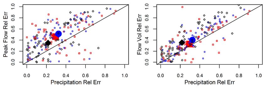
Geosciences 2018, 8, 191 10 of 18
In general, the satellite products (adjusted and unadjusted) underestimated the storm events from
the stage IV record at all spatial scales with the exception of some storm events. This is not surprising
given the small sample size focused on events on the tail side of the distribution. Other researchers
have noted similar satellite underestimations for high magnitude events [14–16,56]. However, it should
be noted there was no strong correlation between percent bias and total accumulated precipitation
for any of the three spatial domains. Moreover, satellite-based products underestimated heavy storm
events in larger spatial domains (0.4 to 1.3 million km2 ) in several regions of Africa [11].
Generally, the satellite-based precipitation products showed less variability in the case of the
Guadalupe basin (Large) relative to the two smaller watersheds (Figure 4). This could be mainly
because of the smoothing power of mean value over the large spatial domain (filtering the noise
introduced by the products). Both products from CMOPRH (labeled as CM and CM 8K) showed very
high correlation with the stage IV product in all spatial domains with very high Nash coefficient. GPM
Early was found to be inconsistent with a very high variance of Nash coefficient in all spatial domains,
however, the variance was decreased as the watershed size increase. Surprisingly, TRMM showed a
very high variance in all the performance statics, especially in the two small watersheds. In contrast,
the TRMM-RT product showed relatively better performance. As described above, the performance
of GPM Final product was inferior to the earlier ones. The whole distribution of the performance
statistics
Geosciencesis2018,
provided
8, x FORin Figure
PEER 4.
REVIEW 10 of 17
Figure4.4.Boxplots
Figure Boxplotsfor
forhyetograph
hyetographperformance
performancestatistics
statisticsfor
forall
allspatial
spatialdomains.
domains.X-axis
X-axislabels
labelsare
are
abbreviatedasasfollows:
abbreviated follows:TRMM—TRMM
TRMM—TRMM3B42, 3B42,CM—CMORPH
CM—CMORPHCDR, CDR,GPM
GPMF—GPM
F—GPMIMERG IMERGFINAL,
FINAL,
CM8K—CMORPH
CM 8K—CMORPH8KM, 8KM,PER
PERC—PERSIANN
C—PERSIANNCCS, CCS,GPM
GPME—GPME—GPMIMERGIMERGEARLY,
EARLY,GPM GPML—GPM
L—GPM
IMERGLATE,
IMERG LATE,CM CMRAW—CMORPH
RAW—CMORPHRAW, RAW,TRMM-RT—TRMM-RT
TRMM-RT—TRMM-RT3B42, 3B42,and
andPER—PERSIANN.
PER—PERSIANN.
Boxplotsdisplay
Boxplots displaythe
thelower
lowerand
andupper
upperquartiles
quartilesand
andmedian.
median.Whiskers
Whiskersextend
extendtotothe
thedata
datapoint
pointnearest
nearest
±± 1.5
1.5 ** interquartile
interquartilerange.
range.
Table to
In order 3. Satellite
providehyetograph performance
some comparison statistics
between aggregated
satellites across the
products, three spatialstatistic
performance domains.results
were pooled from Gauge all spatial
Correctiondomains for each individual satelliteNo product. Table 3 displays the
Gauge Correction
GPM CMORPH PERSIANN GPM GPM CMORPH TRMM-
◦ uncorrected
median, average,TRMM and range CMORPH of theFINAL
statistics8KM
after this CCS
aggregation.
EARLY For the
LATE 0.25 RAW RT products,
PERSIANN
performance PBIASstatistics
−3.9 indicated
−2.9 CMORPH
−51.9 0.2 RAW >−28.2 TRMM-RT −30.4 > PERSIANN
−17.6 −12.2 for the
−14.2nine events
−39.7
nRMSE 58.2 29.5 111.2 31.4 66.9 83.5 57.3 72.3 79.3 84.1
examined.
Average Sapiano
NSE 0.42 and 0.89Arkin [10]−0.32 found 0.87 that correlations
0.38 were highest
0.01 0.62 with CMORPH
0.32 0.26 in
0.06 an
PBIAS −4.4 −7.0 −54.1 −4.6 −29.7 −40.3 −24.3 −24.7 −37.2 −46.3
inter-comparison
nRMSE and
48.0 validation
26.9 study
117.8 on sub-daily
28.0 satellite
59.8 precipitation
88.7 57.2 data. For
67.9 the gauge
73.2 corrected
90.0
products 0.25◦ , there
Median atNSE 0.77 was0.93very little
−0.40 difference
0.92 between0.63 TRMM 0.16and CMORPH
0.64 when the
0.53 0.45same events
0.18
PBIAS 143.1 69.3 32.1 84.3 132.5 74.8 54.0 140.4 135.2 134.0
were compared
nRMSE (2015
210.7 events 56.5 unavailable
63.5 for
54.7CMORPH). 153.2 It is difficult
138.2 to draw140.9
56.1 conclusions
123.0 about the
176.0
Range NSE 5.0 0.4 1.4 0.5 2.9 2.4 0.7 2.3 2.4 3.9
Count 27 21 6 21 27 6 6 27 27 27
3.2. Impact of Spatial Resolution
Several papers have noted a scale dependence of error caused by the inability of coarse-Geosciences 2018, 8, 191 11 of 18
performance of GPM given that only two events were measured. GPM results are compared to the
other products for the 2015 events below.
Table 3. Satellite hyetograph performance statistics aggregated across the three spatial domains.
Gauge Correction No Gauge Correction
GPM CMORPH PERSIANN GPM GPM CMORPH
TRMM CMORPH TRMM-RT PERSIANN
FINAL 8KM CCS EARLY LATE RAW
PBIAS −3.9 −2.9 −51.9 0.2 −28.2 −30.4 −17.6 −12.2 −14.2 −39.7
nRMSE 58.2 29.5 111.2 31.4 66.9 83.5 57.3 72.3 79.3 84.1
Average NSE 0.42 0.89 −0.32 0.87 0.38 0.01 0.62 0.32 0.26 0.06
PBIAS −4.4 −7.0 −54.1 −4.6 −29.7 −40.3 −24.3 −24.7 −37.2 −46.3
nRMSE 48.0 26.9 117.8 28.0 59.8 88.7 57.2 67.9 73.2 90.0
Median NSE 0.77 0.93 −0.40 0.92 0.63 0.16 0.64 0.53 0.45 0.18
PBIAS 143.1 69.3 32.1 84.3 132.5 74.8 54.0 140.4 135.2 134.0
nRMSE 210.7 56.5 63.5 54.7 153.2 138.2 56.1 140.9 123.0 176.0
Range NSE 5.0 0.4 1.4 0.5 2.9 2.4 0.7 2.3 2.4 3.9
Count 27 21 6 21 27 6 6 27 27 27
3.2. Impact of Spatial Resolution
Several papers have noted a scale dependence of error caused by the inability of coarse-resolution
products to adequately represent mean areal precipitation in smaller basins because their sampling
involves an area much larger than the basin (e.g., Nikolopoulos, Anagnostou [14]). Here, we investigate
the scale dependence of rainfall error first by comparing the CMORPH and PERSIANN products with
their fine-scale counterparts and then by examining changes in PBIAS as a function of watershed size.
The PERSIANN CCS product has a spatial resolution of 0.04 degrees and has a similar size to
stage IV bins across the study area. When compared to PERSIANN, the PERSIANN CCS product
consistently performed better in each of the three watersheds for all performance statistics. However,
the gap in performance statistics did not grow as watershed size decreased, as may be expected if
scale issues were the root cause of the discrepancy. It is difficult to identify the primary causes for the
differing performance given PERSIANN CCS uses different processing algorithms.
Unlike the PERSIANN products, there was virtually no difference between CMORPH and
the CMORPH 8KM product with regard to performance statistics. This suggests the downscaling
techniques employed by the CMORPH 8KM product are not adequate if their intent is to provide a
more detailed spatial representation of rainfall.
3.3. GPM Rainfall Events
The two largest rain events from the dataset occurred in May and October of 2015, and both
resulted in significant flash flood events along the Blanco River [42]. These events were captured by
GPM and offer an initial look at GPM performance for short duration high magnitude storms. Figure 5
shows performance statistic results for each of the real-time products (PERSIANN, PERSIANN-CCS,
TRMM-RT, and CMORPH RAW) along with the Early and Late GPM runs. Generally, the GPM
products performed better than did the other real-time satellite products. For the May 2015 event,
the Early product produced better estimates than the Late run, with the opposite pattern for the
October 2015 event. Gauge corrected estimates (Table 3) showed a significant underestimation of the
events, which is not surprising given it is adjusted to monthly values. The Early GPM product failed to
capture the storm event of October 2015 showed by the negative value of Nash coefficient (Figure 5).
As anticipated, hydrograph results closely mimic the rainfall fields with respect to their ability to
overestimate and underestimate the reference Stage IV forcing. The hydrographs driven by Stage IV
rainfall along with satellite results for the nine storm events at the Guadalupe basin outlet are shown
in Figure 6 (same as Figure 3). The hydrographs from the products were able to capture the bi-modal
behavior of the hydrograph but with a high range of accuracy levels for November 2004 and May
2014 events. Some of the errors were quite high, indicating that the rainfall errors were amplified in
the resulting runoff hydrograph. In the case of the events that have a one peak hydrograph, most
of the products tend to underestimate the hydrograph by a considerable amount. As expected, thein May, the magnitude and the pattern of the stage IV seem to be the mean value of the hydrographs
from the satellite-based products.
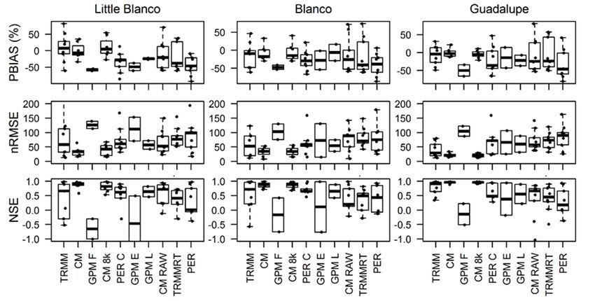
The performance of the precipitation products in the simulated hydrograph followed a similar
pattern as described in the precipitation analysis. However, the variability of the products seems to
increase 2018,
Geosciences as the scale of the watershed increases. Boxplot results showing performance statistics
8, 191 at
12 of 18
each of the three basins are displayed in Figure 7. The CMORPH product (labeled as CM) showed
higher Nash coefficient in Little Blanco (the smallest basin) but as the size of the watershed increased,
hydrographs
the performance drivenwasby thetoGPM
seen Early and
plummet. Late products
A similar hadobserved
pattern was less errors
in than
mostthose driven by
the products the
when
Final products due to the severe underestimation of rainfall by the latter as described
moving from Little Blanco to Guadalupe. All evaluation criteria showed a very wide range and high above (see
Figures
variability3 and
and 4). Inmagnitude
error all the fall in
events, theofpattern
the case of the hydrograph
the Guadalupe Basin (Figurewas more
7). The or less captured,
accumulated effect
but with very significant underestimation of the precipitation. For the events
of all the discrepancies in the products across the watershed caused a significant increase that occurred in May,in
the
variability at the outlet. However, the increase in spatial domain of the watershed improved the
magnitude and the pattern of the stage IV seem to be the mean value of the hydrographs from the
satellite-based
performance ofproducts.
the GPM Late product across all the criteria.
Figure 5.
Figure 5. Performance
Performance statistic
statistic results
results for the non-gauge
for the non-gauge adjusted
adjusted satellite
satellite results for the
results for the May
May and
and
October 2015
October 2015 storms
storms that
that included
included the
the GPM
GPM products.
products.
Geosciences 2018, 8, x FOR PEER REVIEW 12 of 17
Figure
Figure6.6.Streamflow
Streamflowhydrographs
hydrographsatatthe
theBlanco
Blancowatershed
watershedoutlet.
outlet.Legend
Legendlabels
labelsare
areabbreviated
abbreviatedas
as
follows:
follows: MPE—Stage IV, TRMM—TRMM 3B42, CM—CMORPH CDR, GPM F—GPM IMERGIMERG
MPE—Stage IV, TRMM—TRMM 3B42, CM—CMORPH CDR, GPM F—GPM FINAL,
FINAL, CM 8K—CMORPH
CM 8K—CMORPH 8KM,
8KM, PER PER C—PERSIANN
C—PERSIANN CCS,
CCS, GPM GPM E—GPM
E—GPM IMERG EARLY,
IMERG EARLY, GPM L—GPMGPM
L—GPM IMERG LATE, CM RAW—CMORPH RAW, TRMM-RT—TRMM-RT
IMERG LATE, CM RAW—CMORPH RAW, TRMM-RT—TRMM-RT 3B42, and PER—PERSIANN. 3B42, and PER—
PERSIANN.Geosciences 2018, 8, 191 13 of 18
The performance of the precipitation products in the simulated hydrograph followed a similar
pattern as described in the precipitation analysis. However, the variability of the products seems to
increase as the scale of the watershed increases. Boxplot results showing performance statistics at
each of the three basins are displayed in Figure 7. The CMORPH product (labeled as CM) showed
higher Nash coefficient in Little Blanco (the smallest basin) but as the size of the watershed increased,
the performance was seen to plummet. A similar pattern was observed in most the products when
moving from
Figure Little Blanco
6. Streamflow to Guadalupe.
hydrographs at theAll evaluation
Blanco criteria
watershed outlet.showed
Legend alabels
veryare
wide range and
abbreviated as high
variability and
follows: error magnitude
MPE—Stage in the case of the
IV, TRMM—TRMM Guadalupe
3B42, CM—CMORPH Basin (Figure
CDR, GPM7). The accumulated
F—GPM IMERGeffect
of allFINAL,
the discrepancies
CM 8K—CMORPH 8KM, PER C—PERSIANN CCS, GPM E—GPM IMERG EARLY, variability
in the products across the watershed caused a significant increase in GPM
at theL—GPM
outlet. However,
IMERG LATE,the increase in spatial domain
CM RAW—CMORPH of the
RAW, watershed improved
TRMM-RT—TRMM-RT the performance
3B42, and PER— of
the GPM Late product across all the criteria.
PERSIANN.
Figure 7.
Figure 7. Boxplots
Boxplots for hydrograph performance
for hydrograph performance statistics
statistics for
for all
all spatial
spatial domains.
domains. X-axis
X-axis labels
labels
representations are
abbreviations and boxplot representations are the
the same
same asas those
those described
describedin inFigure
Figure4.4.
3.4. GPM
3.4. GPM Model
Model Simulations
Simulations
GPM products
GPM products showed
showed aa higher
higher Nash
Nash Coefficient
Coefficient thanthan their
their counterparts
counterparts in both events
in both events in
in all
all
spatial scales except in the case of Little Blanco for the May 2015 event. Moreover,
spatial scales except in the case of Little Blanco for the May 2015 event. Moreover, the Late GPM the Late GPM
product outclassed
product outclassedthe
theEarly
EarlyGPM
GPMproduct
productininalmost
almostallallthe
thecriteria
criteriaand
and
ininallall spatial
spatial domains.
domains. There
There is
is no clear pattern of the impact of scale effect on a single product but, in case of
no clear pattern of the impact of scale effect on a single product but, in case of GPM products, GPM products, the
the performance of the PBIAS was improved as the spatial domain increased. However, the variability
of the performance of the non-gauge adjusted products increased as the spatial domain size increased
(Figure 8).Geosciences
Geosciences 2018,
2018, 8,
8, xx FOR
FOR PEER
PEER REVIEW
REVIEW 13
13 of
of 17
17
performance
performance of of the
the PBIAS
PBIAS was
was improved
improved as
as the
the spatial
spatial domain
domain increased.
increased. However,
However, the
the variability
variability
of
of the
the performance
2018, 8, 191 of
performance
Geosciences of the
the non-gauge
non-gauge adjusted
adjusted products
products increased
increased as
as the
the spatial
spatial domain
domain size
size increased
increased
14 of 18
(Figure 8).
(Figure 8).
Figure
Figure 8.
Figure 8. Performance
8. Performance statistic
Performance statistic results
statistic results for
results for the
for the non-gauge
the non-gauge adjusted
non-gauge adjusted satellite
adjusted satellite results
satellite results for
results for the
for the May
the May and
May and
and
October
October 2015
2015 storms
storms that
that included
included the
the GPM
GPM products
products (for
(for the
the hydrographs).
hydrographs).
October 2015 storms that included the GPM products (for the hydrographs).
3.5.
3.5. Error
Error Propagation
Propagation
3.5. Error Propagation
The
The error
error was
was seen
seen to
to propagate
propagate from from the
the precipitation
precipitation dataset
dataset to to the hydrograph at the outlet.
The error was seen to propagate from the precipitation dataset to the
the hydrograph
hydrograph at at the
the outlet.
outlet.
The
The propagation
propagation was
was magnified
magnified in
in all
all of
of the
the criteria
criteria shown
shown in
in Figure
Figure 9
9 except
except in
in the
the case
case of
of the
the
The propagation was magnified in all of the criteria shown in Figure 9 except in the case of the
streamflow
streamflow PBIAS.
PBIAS. Moreover,
Moreover, the
the pattern
pattern was
was seen
seen across
across all
all the
the spatial
spatial domains
domains in
in the
the same
same manner.
manner.
streamflow PBIAS. Moreover, the pattern was seen across all the spatial domains in the same manner.
The scale
The scale effect
scaleeffect
effectofof the
ofthe spatial
thespatial
spatial domains
domains does
does not seem to
to affect the error propagation, as
as they were
The domains does notnot
seemseem affect
to affect the the
errorerror propagation,
propagation, as they they
were were
very
very
very close
close in
in all
all the
the evaluation
evaluation criteria
criteria (Figure
(Figure 9).
9).
close in all the evaluation criteria (Figure 9).
Figure
Figure 9.9. Annual
Annual Error propagations descriptions
Error propagations descriptions comparing
comparing streamflow
comparing streamflow and and precipitation
precipitation percent
percent
bias (PBIAS)
(PBIAS)
bias (PBIAS) and
and normalized
normalized root-mean-square-error
root-mean-square-error (nRMSE)
(nRMSE)
(nRMSE) (top
(top left
left and
and top
top right,
right, respectively)
respectively)
and relative
and relative error
errorinin
relativeerror precipitation
precipitation
in versus
versus
precipitation peak
versus peak
flowflow
peak relative
relative
flow error error
relative error (bottom
(bottom left)
left) and
(bottom and
and streamflow
streamflow
left) volume
streamflow
volume
relative relative
volume error error
error (bottom
(bottom
relative right)
right) N.B.
(bottom the N.B.
right) the
the big
big markers
N.B. big markers
representrepresent
markers the meanthe
represent mean
mean value.
value.
the value.
4.
4. Conclusions
ConclusionsGeosciences 2018, 8, 191 15 of 18
4. Conclusions
Precipitation is the main driver of all the hydrologic models that are used to predict/forecast the
relationship between rainfall and runoff. Moreover, rainfall amount and distribution represent the
major components of the floodplain analysis and water resource management practices. That is why
it is a significant achievement to capture the spatial and temporal distribution of rainfall, since the
accuracy of almost all hydrologic processes depends on the accuracy of the precipitation estimates.
Rain gauges are only reliable for a very small area because of the intermittent behavior of precipitation.
Radars have problems with beam blockage in complex terrain and lack even distribution across the
globe. Satellite-based precipitation estimation with high spatiotemporal resolution has a potential to
capture the spatiotemporal distribution of precipitation if the products and algorithms are improved
to a reasonable accuracy.
The assessment of ten satellite-based precipitation products was carried in relation to the radar
stage IV (NCEP product) over Guadalupe river basin with a drainage area of around 9000 km2 .
Moreover, the assessment was done in two smaller sub-watersheds of the Guadalupe river basin (Little
Blanco River (178 km2 ) and the Blanco River (1130 km2 )). This procedure was done to assess the scale
impact on the accuracy of the products. Nine significantly large events with a wide spatial coverage
were used in the analysis.
Furthermore, to understand the propagation of rainfall error into the predicted runoff, hydrologic
model simulations were implemented. GSSHA, a physically-based fully distributed hydrologic model,
forced with those ten satellite-based precipitation products, was used to simulate the rainfall-runoff
relationship for the basins. The most widely used model evaluation criteria such as Nash-Sutcliffe,
PBIAS, nRMSE, and relative error were used in the assessment of both precipitation and hydrographs
of the outlet.
The products underestimated the storm events in relation to the radar product Stage IV.
This pattern was seen in several other studies over various regions of the world [14–16,56]. Moreover,
the satellite-based precipitation products showed a very compact distribution in all the evaluation
criteria in the case of the largest basin. Both products of CMORPH showed a very high correlation in
all spatial domains and was reflected with an average Nash-Sutcliffe coefficient of 0.81. GPM Early
was found to be inconsistent with a very high variance of Nash coefficient in all spatial domains (from
−0.46 to 0.38), however, the variance was decreased as the watershed size increased. This is mainly
due to the smoothing caused by averaging over a larger area. Among all GPM products, the Final
product underestimated rainfall most, indicating that the methodology used to prepare the product
(using climatology and rain gauges) probably was not able to capture the areas and/or periods of very
intense localized rainfall. Surprisingly, TRMM also showed a very high variance in all the performance
statics, especially in the two small watersheds (from −4.0 to 0.99 with an average of 0.16). In contrast,
the TRMM RT (non-gauge corrected product of TRMM) product showed relatively better performance
of Nash-Sutcliffe with an average of 0.39 and a range from 0.05 to 0.82.
The pattern of the precipitation estimates was also reflected on the simulated hydrograph forced
by the precipitation products. The average Nash-Sutcliffe coefficient was reduced from 0.81 in
precipitation to 0.58 in the runoff for CMORPH. CMORPH product showed higher Nash coefficient
in Little Blanco (the smallest basin) but as the size of the watershed increased, the performance was
seen to plummet. A similar pattern was observed in most of the products when moving from Little
Blanco to Guadalupe. However, the increase in the spatial domain of the watershed improved the
performance of the GPM Late product across all the criteria.
The error was seen to amplify as it propagated from the precipitation dataset to the hydrograph
at the outlet. The propagation was magnified in all of the evaluation criteria except in the case of the
streamflow PBIAS. Moreover, the pattern was seen across all the spatial domains in the same manner.
The scale effect of the spatial domains does not seem to affect the error propagation as it was very close
in all of the evaluation criteria.Geosciences 2018, 8, 191 16 of 18
In summary, the satellite-based precipitation products provide very high spatiotemporal
resolution precipitation estimates. However, the estimates lack accuracy, especially at a local scale.
The products underestimate heavy storm events significantly, and the errors were amplified in the
runoff hydrographs generated.
Author Contributions: H.O.S. and C.F. designed the overall study. C.F. downloaded the remote sensing products
and prepared and performed the hydrologic model simulations with input from H.O.S. D.G. helped C.F. with
post-analysis of the model outputs and preparation of the first draft. C.F. and H.O.S. reviewed and revised the
manuscript. H.O.S. did the final overall proofreading of the manuscript.
Funding: This research was funded by U.S. Army Research Office (Grant W912HZ-14-P-0160).
Acknowledgments: This research funded in part by the U.S. Army Research Office (Grant W912HZ-14-P-0160).
This support is cordially acknowledged.
Conflicts of Interest: The authors declare no conflict of interest.
References
1. Dai, A. Precipitation Characteristics in Eighteen Coupled climate models. J. Clim. 2006, 19, 4605–4630.
[CrossRef]
2. New, M.; Todd, M.; Hulme, M.; Jones, P. Precipitation measurements and trends in the twentieth century.
Int. J. Clim. 2001, 21, 1889–1922. [CrossRef]
3. Krajewski, W.; Smith, J. Radar hydrology: Rainfall estimation. Adv. Water Resour. 2002, 25, 1387–1394.
[CrossRef]
4. Wang, X.; Xie, H.; Sharif, H.; Zeitler, J. Validating NEXRAD MPE and Stage III precipitation products for
uniform rainfall on the Upper Guadalupe River Basin of the Texas Hill Country. J. Hydrol. 2008, 348, 73–86.
[CrossRef]
5. Habib, E.; Larson, B.F.; Graschel, J. Validation of NEXRAD multisensor precipitation estimates using an
experimental dense rain gauge network in south Louisiana. J. Hydrol. 2009, 373, 463–478. [CrossRef]
6. Maddox, R.A.; Zhang, J.; Gourley, J.J.; Howard, K.W. Weather radar coverage over the contiguous United
States. Weather Forecast. 2002, 17, 927–934. [CrossRef]
7. Nicholson, S.E.; Some, B.; McCollum, J.; Nelkin, E.; Klotter, D.; Berte, Y.; Diallo, B.M.; Gaye, I.; Kpabeba, G.;
Ndiaye, O.; et al. Validation of TRMM and other rainfall estimates with a high-density gauge dataset for
West Africa. Part II: Validation of TRMM rainfall products. J. Appl. Meteorol. 2003, 42, 1355–1368. [CrossRef]
8. McCollum, J.R.; Krajewski, W.F.; Ferraro, R.R.; Ba, M.B. Evaluation of biases of satellite rainfall estimation
algorithms over the continental United States. J. Appl. Meteorol. 2002, 41, 1065–1080. [CrossRef]
9. Ebert, E.E.; Janowiak, J.E.; Kidd, C. Comparison of near-real-time precipitation estimates from satellite
observations and numerical models. Bull. Am. Meteorol. Soc. 2007, 88, 47–64. [CrossRef]
10. Sapiano, M.; Arkin, P. An intercomparison and validation of high-resolution satellite precipitation estimates
with 3-hourly gauge data. J. Hydrometeorol. 2009, 10, 149–166. [CrossRef]
11. Thiemig, V.; Rojas, R.; Zambrano-Bigiarini, M.; Levizzani, V.; de Roo, A. Validation of satellite-based
precipitation products over sparsely gauged African river basins. J. Hydrometeorol. 2012, 13, 1760–1783.
[CrossRef]
12. Hirpa, F.A.; Gebremichael, M.; Hopson, T. Evaluation of high-resolution satellite precipitation products over
very complex terrain in Ethiopia. J. Appl. Meteorol. Climatol. 2010, 49, 1044–1051. [CrossRef]
13. Mantas, V.; Liu, Z.; Caro, C.; Pereira, A.J.S.C. Validation of TRMM multi-satellite precipitation analysis
(TMPA) products in the Peruvian Andes. Atmos. Res. 2015, 163, 132–145. [CrossRef]
14. Nikolopoulos, E.I.; Anagnostou, E.N.; Hossain, F.; Gebremichael, M.; Borga, M. Understanding the scale
relationships of uncertainty propagation of satellite rainfall through a distributed hydrologic model.
J. Hydrometeorol. 2010, 11, 520–532. [CrossRef]
15. AghaKouchak, A.; Behrangi, A.; Sorooshian, S.; Hsu, K.; Amitai, E. Evaluation of satellite-retrieved extreme
precipitation rates across the central United States. J. Geophys. Res. Atmos. 2011, 116. [CrossRef]
16. Mehran, A.; AghaKouchak, A. Capabilities of satellite precipitation datasets to estimate heavy precipitation
rates at different temporal accumulations. Hydrol. Process. 2014, 28, 2262–2270. [CrossRef]You can also read