Using global variance-based sensitivity analysis to prioritise bridge retrofits in a regional road network subject to seismic hazard
←
→
Page content transcription
If your browser does not render page correctly, please read the page content below
Bhattacharjee, G., and Baker, J. W. (2021). “Using global variance-based sensitivity analysis to
prioritise bridge retrofits in a regional road network subject to seismic hazard.” Structure and
Infrastructure Engineering (in press).

 Using global variance-based sensitivity analysis to prioritise bridge
   retrofits in a regional road network subject to seismic hazard
                             Gitanjali Bhattacharjee, Jack W. Baker

Abstract
This paper presents a novel method for prioritising bridge retrofits within a regional road network
subject to uncertain seismic hazard, using a technique that accounts for network performance while
avoiding the combinatoric computational costs of exhaustive searches. Using global variance-based
sensitivity analysis, a probabilistic ranking of bridges is determined according to how much their
retrofit statuses influence the expected cost of the road network disruption. Bridges’ total-order
sensitivity (Sobol’) indices are estimated with respect to the expected cost using the hybrid-point
Monte Carlo approximation method. A bridge’s total-order Sobol’ index measures how much its
retrofit status influences the variance of the expected cost of the road network performance and
accounts for the effect of its interactions with other bridges’ retrofit states. For 71 highway bridges
in San Francisco, a retrofit strategy based on bridges’ total-order Sobol’ indices outperforms other
heuristic strategies. The proposed method remains computationally tractable while accounting for
the probabilistic nature of the seismic hazard, the uniqueness of individual bridges, network effects,
and decision-makers’ priorities. Because this method leverages existing risk assessment tools and
models without imposing further assumptions, it should be extensible to other types of networks
under different types of hazards and to other decision variables.

Keywords: transportation networks, sensitivity analysis, risk management, retrofitting, earth-
quake engineering, decision making

1    Introduction
This paper presents a novel method for prioritising bridge retrofits within a regional road network
subject to uncertain seismic hazard, using a technique that accounts for network effects and dis-
ruptions while avoiding the combinatoric computational costs of exhaustive searches. This method
uses global variance-based sensitivity analysis (SA) to compute a probabilistic ranking of bridges
according to how much their retrofit status influences the decision variable of interest. The pro-
posed method is demonstrated on a network of B = 71 unique bridges in the San Francisco Bay
Area for two decision variables of interest: (1) the expected cost of the road network performance
(2) the ratio of the cost of bridge seismic retrofits to the expected cost of the road network per-
formance. The performance of the proposed method is compared to that of other heuristic retrofit
prioritisation strategies.

    The key contribution of this research is in providing a flexible decision-support tool with which
to manage risks to complex, real-world networks. The proposed SA-based retrofit prioritisation
method builds upon existing event-based probabilistic hazard frameworks that include a set of po-
tential seismic scenarios, described by magnitudes and occurrence rates established using seismic

                                                  1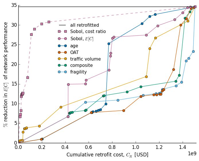
Bhattacharjee, G., and Baker, J. W. (2021). “Using global variance-based sensitivity analysis to
prioritise bridge retrofits in a regional road network subject to seismic hazard.” Structure and
Infrastructure Engineering (in press).

risk assessment procedures. This method leverages existing tools and models without imposing
further assumptions – it should therefore be extensible to other types of networks under different
types of hazards and with consideration given to different decision-makers’ priorities.

    This paper is organised as follows: Section 2 reviews pre-earthquake bridge seismic retrofit
prioritisation strategies, Section 3 introduces the proposed bridge retrofit prioritisation method,
Section 4 presents an example application to illustrate the proposed method and compare its
performance with that of other heuristic retrofit strategies, Section 5 provides further discussion of
how to implement the proposed method, and Section 6 gives conclusions.

2    Background
Road networks are lifelines and play an important role in everyday life as well as in response and
community recovery after an earthquake, as they enable repairs to other lifelines (Frangopol &
Bocchini, 2012). Bridges are often the most fragile components of road networks subject to seis-
mic hazard, and bridge damage due to earthquakes can be costly (e.g., Gordon, Richardson, &
Davis, 1998). Retrofitting is an effective method of mitigating the risk of bridge damage due to
earthquakes (e.g., Giovinazzi et al., 2011). Deciding which bridges within a large road network to
retrofit to meet a particular system performance objective remains a challenging problem, due to
the size and complexity of the road network, the large number of possible retrofit combinations,
and the number of earthquake rupture scenarios that must be considered to describe the regional
seismic hazard (Gomez & Baker, 2019).

    Approaches to pre-earthquake bridge seismic retrofit prioritisation can be broadly categorised
as heuristic or optimization-based. Heuristic approaches prioritise bridges for retrofit accord-
ing to an importance measure. Characteristic-based, conditional, reliability-based, and network
topology-based importance measures constitute four classes of commonly used importance mea-
sures. Characteristic-based importance measures are the least computationally expensive, as they
rely only on information about an individual bridge’s particular characteristics, such as the average
number of vehicles that pass over it in a day (e.g., Buckle et al., 2006; Miller, 2014). More so-
phisticated characteristic-based importance measures like the indices method proposed by Buckle
et al. (2006) combine multiple criteria, including bridges’ structural characteristics, socioeconomic
importance, and site seismic characteristics (Buckle et al., 2006; Sims, 2000). Buckle et al. (2006)
also proposed the expected damage method, which involves assessing the severity of the expected
damage of each bridge in the road network for a single earthquake, and the seismic risk assessment
method, which involves estimating the effect on system performance of bridge damage for a given
hazard level. Rokneddin (2013) extends the expected damage method of Buckle et al. (2006) to ac-
count for how bridge fragilities change with time by ranking bridges using time-dependent fragility
analysis. These prioritisation methods do not take into account the topology or performance of the
road network and assess bridges independently of one another.

    Conditional importance measures quantify the probability that a system component has failed
given that the system as a whole has failed, and are generally applicable to infrastructure network
components (Rokneddin, 2013; Song & Kiureghian, 2005). They allow the analyst to include some
measure of network performance when assessing the importance of individual components in the
network. Basic conditional importance measures include the risk achievement worth (RAW), risk
reduction worth (RRW), and boundary probability (BP), each of which estimates the sensitivity

                                                  2
Bhattacharjee, G., and Baker, J. W. (2021). “Using global variance-based sensitivity analysis to
prioritise bridge retrofits in a regional road network subject to seismic hazard.” Structure and
Infrastructure Engineering (in press).

of a system’s failure probability to the states of its constituent components – when a component is
damaged (RAW), when a component is invulnerable (RRW), and when a component is upgraded
(BP) (Dutuit & Rauzy, 2015; Song & Kiureghian, 2005). Barker, Ramirez-Marquez, and Rocco
(2013) propose two variants of the RAW and RRW that incorporate a measure of network resilience.
RAW, RRW, and BP do not account for the vulnerability of the network components to damage,
nor any dependencies that might exist between them, and are computed in a deterministic setting,
thus neglecting key features of an infrastructure network (Borgonovo & Plischke, 2016; Frangopol
& Bocchini, 2012; Miller, 2014; Song & Kiureghian, 2005). Because they require estimation of both
system and component failure probabilities, conditional importance measures may be expensive to
compute compared to other importance measures (Rokneddin, 2013; Song & Kiureghian, 2005).
Miller (2014) proposes a composite importance measure to classify bridges for preliminary retrofit
screening according to how frequently they appear in damage maps that result in high losses in
network performance. The composite importance measure is probabilistic and can capture non-
linearities in the road network performance that result from simultaneous bridge failures .

     Moghtaderi-Zadeh and Kiureghian (1983) develop a geometric method for efficiently identifying
“critical” components (whether nodes or edges) of large lifeline networks exposed to seismic hazard.
Small changes in the strength of these critical components produce significant changes to the net-
work’s reliability (Moghtaderi-Zadeh & Kiureghian, 1983). M. Liu and Frangopol (2005) formulate
the reliability importance factor of a bridge in a road network as the ratio of the change in reliability
of the road network when a bridge’s reliability changes to that of the change in the reliability of the
individual bridge. Their formulation is intended to prioritise bridges for maintenance rather than
retrofit and does not take into account seismic hazard (M. Liu & Frangopol, 2005). The random
forests importance measure proposed by Rokneddin (2013) accounts for bridges’ vulnerability and
their roles in the larger road network and results in a probabilistic ranking, but does not account
for the performance of the road network in terms of congestion. Another approach to quantify the
importance of different bridges in a road network is to adapt metrics from classic network anal-
ysis, such as bridges’ betweenness centrality (e.g., Rokneddin, Ghosh, Dueñas-Osorio, & Padgett,
2013). Rokneddin (2013) also proposes BridgeRank, which combines a bridge’s topological impor-
tance with its fragility to determine its importance within the road network. BridgeRank does
not account for network performance or multiple earthquake scenarios, though it does consider the
network topology (Rokneddin, 2013).

    The computational tractability of importance measures for large infrastructure networks comes
at the expense of other desirable characteristics, among them that an importance measure should
account for the likelihood of bridge damage in different scenarios, the performance of the road net-
work, and the effects of multiple bridge failures. Most of the importance measures discussed above
sacrifice at least one of these qualities. Furthermore, most importance measures account only for
the effects of bridge damage and neglect to model the effects of bridge retrofits; none incorporate
budgetary constraints.

    Optimisation-based approaches select a subset of bridges within a road network to retrofit
such that a user-defined objective is met and guarantee a solution with some degree of optimality.
Two-stage stochastic programs are popular in infrastructure risk management literature (Grass &
Fischer, 2016) and allow for simultaneous consideration of pre- and post-earthquake decisions, i.e.,
retrofit and repair, as well as budgetary constraints (Barbarasoglu & Arda, 2004; Fan, Liu, Lee, &
Kiremidjian, 2010; Gomez & Baker, 2019; C. Liu, Fan, & Ordóñez, 2009; Miller-Hooks, Zhang, &
Faturechi, 2012; Peeta, Sibel Salman, Gunnec, & Viswanath, 2010). Optimisation-based approaches

                                                   3
Bhattacharjee, G., and Baker, J. W. (2021). “Using global variance-based sensitivity analysis to
prioritise bridge retrofits in a regional road network subject to seismic hazard.” Structure and
Infrastructure Engineering (in press).

also offer flexibility in terms of decision-makers’ priorities: objective functions include measures of
road network sustainability (Dong, Frangopol, & Saydam, 2014), reliability (Zhang & Wang, 2016),
resilience (Miller-Hooks et al., 2012), maximum network flow (Chang, Peng, Ouyang, Elnashai, &
Spencer, Jr., 2012), and aggregate retrofit and repair costs (Gomez & Baker, 2019). Optimisation-
based approaches have been demonstrated on smaller systems, but application to large networks
remains challenging. Most have been applied to networks with fewer than 20 bridges (e.g., Dong
et al., 2014; Fan et al., 2010; Peeta et al., 2010), with some notable exceptions: Chang et al.
(2012) consider 616 bridges of the same structural type, and Gomez and Baker (2019) consider 65
unique bridges. Common simplifications include considering one earthquake scenario rather than
conducting a probabilistic analysis (e.g., Chang et al., 2012; Miller-Hooks et al., 2012; Zhang &
Wang, 2016), modelling bridges as having identical structural characteristics (e.g., Chang et al.,
2012), assuming that retrofitted bridges cannot be damaged (e.g., C. Liu et al., 2009), or assuming
that bridges fail independently of one another (e.g., Peeta et al., 2010).

3     Methods
3.1   Global variance-based sensitivity analysis
Saltelli, Tarantola, Campolongo, and Ratto (2004) define sensitivity analysis as “the study of how
the uncertainty in the output of a model . . . can be apportioned to different sources of uncertainty
in the model input”. Local (or deterministic) SA is performed around a particular point of interest
in the model input space, in contrast to global (or probabilistic) SA, which considers the entire
model input space (Borgonovo & Plischke, 2016; Saltelli et al., 2004). A global variance-based SA
aims to attribute the variability in a scalar output quantity of interest q to variability in the nB
input quantities f = [f1 , f2 , ...fnB ] given some function (not necessarily expressible in closed form)
relating the two, g(f ) = q. Equation (1) gives the basic form of a global SA problem.

                                             f → g(f ) → q                                            (1)
     Sensitivity indices quantify the portion of the variability of q associated with an input fb , b ∈
{1, . . . , nB }. Computing the sensitivity indices of a set of inputs requires treating each input as
a random variable by assigning it a distribution. The portion of the variance of q that can be
attributed to an input fb is bounded by the first- and total-order sensitivity indices of fb . The
first-order sensitivity index, given in Equation (2), quantifies how much of the variance in q can
be attributed solely to variance in fb . In Equation (2), {b} denotes a set containing only the input
variable indexed by b.

                                                    V [E[q|f{b} ]]
                                           S 2b =                                                     (2)
                                                        V [q]
    A second-order sensitivity index quantifies how much of the variance in q can be attributed to
variance in fb and a second input, denoted fc , including interactions between those two variables.
An interaction is that part of the response of the output q to the values of fb and fc “that cannot
be expressed as a superposition of effects separately due to” fb and fc (Saltelli et al., 2004). The
total-order sensitivity index of fb , given in Equation (3), is the sum of the first- and all higher-order
sensitivity indices of fb . It quantifies how much of the variance in the output quantity q can be
attributed to variance in the input quantity fb and its interactions with all other input variables,
denoted by the set {b}.

                                                      4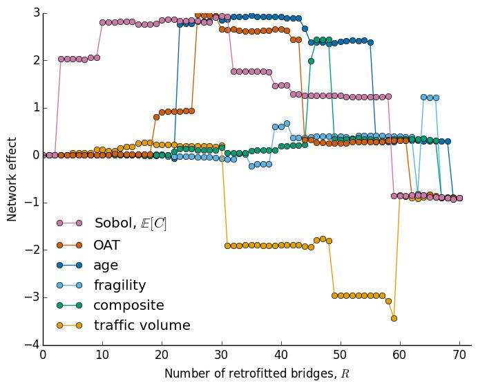
Bhattacharjee, G., and Baker, J. W. (2021). “Using global variance-based sensitivity analysis to
prioritise bridge retrofits in a regional road network subject to seismic hazard.” Structure and
Infrastructure Engineering (in press).

                                              2     E(V [q|f {b} ])
                                             Sb =                                                    (3)
                                                        V [q]
                                                                         2
Both the first and total-order index of fb take values in [0, 1]. S b = 0 indicates that the input fb
is non-influential – i.e., variability in its value does not contribute to variability in the output. It
can therefore be fixed to any value within its distribution without impacting the output variance
(Saltelli et al., 2008). Larger indices indicate that the associated inputs are more influential with
respect to the output.

3.2   Estimation of total-order Sobol’ indices
The total-order sensitivity index in Equation (3) is expensive to compute exactly (Saltelli et al.,
2008). Sobol (1993) developed an estimator for the total-order sensitivity index by using a hybrid-
point Monte Carlo approximation approach, summarised for a set of input variables and function
g(f ) in Algorithm 1. This estimator is referred to as the total-order Sobol’ index.

Algorithm 1 Computing normalised estimated total-order Sobol’ indices for nB input variables.
  procedure ComputeTotalSobolIndices(nB )
     Assign each input variable fb an appropriate distribution
     Sample N vectors, denoted fi , of size nB by sampling each input variable fb independently
     Sample N vectors, denoted fi0 , of size nB by sampling each input variable fb independently
     for b = 1, ..., nB do
           2
        τ̂ b ← 0
        for i = 1, ..., N do
                2                          0 ))2
             τ̂ b + = (g(fi ) − g(fi,b0 : fi,b
                   2
           2    τ̂ b
         τ̂ b ← 2N
         ˆ 2 ← τ̂ 2b
         S                    . This is the normalised total-order Sobol’ index of input variable fb .
           b     σ̂ 2
                 2
             ˆ
      return S                    . This is a vector of n elements in which the bth element is S  ˆ 2.
                                                                 B                                     b

     Equation (4) gives the estimate of the unnormalised total-order Sobol’ index for an input
                             0 denotes the hybrid point, constructed by interleaving elements of the
variable fb , where fi,b0 : fi,b
vectors fi,b0 and fi,b according to to their subscripted index sets: {i, b0 } denotes the realisations of
                    0

all input variables except that indexed by b in the i-th sample of f and {i, b} denotes the realisation
of the input variable indexed by b in the i-th sample of f 0 .
                                             N
                                   2       1 X                      0
                                 τ̂ b =        (g(fi ) − g(fi,b0 : fi,b ))2                          (4)
                                          2N
                                              i=1

      Equation (5) gives the estimate of the normalised total-order Sobol’ index for an input variable
fb , obtained by dividing the unnormalised estimate by the sample variance σ̂ 2 , as given in Equation
(6). Equation (7) computes the sample mean, needed in Equation (6).
                                                            2
                                                    ˆ 2 = τ̂ b
                                                    S                                                (5)
                                                      b
                                                          σ̂ 2

                                                        5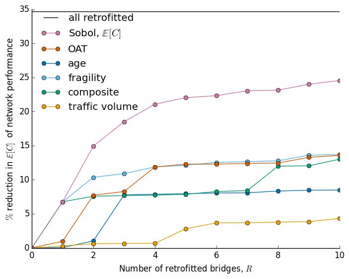
Bhattacharjee, G., and Baker, J. W. (2021). “Using global variance-based sensitivity analysis to
prioritise bridge retrofits in a regional road network subject to seismic hazard.” Structure and
Infrastructure Engineering (in press).

                                                      N
                                                1 X
                                     σ̂ 2 =        (g(fi ) − µ̂)2                                (6)
                                              N −1
                                                     i=1
                                                     N
                                                   1 X
                                              µ̂ =     g(fi )                                    (7)
                                                   N
                                                      i=1

3.3     Bridge retrofit prioritization as a sensitivity analysis problem
Given a set of nB bridges and a limited number of retrofits R < nB to allocate among them, the
objective is to retrofit the bridges whose improved performance results in the greatest improvement
in the performance of the road network. This requires modeling both bridge seismic retrofit and
road network performance, detailed in this section, and formulating the SA problem. The proposed
method is agnostic to the particular measure of road network performance used, which should
reflect the priorities of the analyst using the proposed method to inform a retrofit prioritisation
policy. In this paper, the road network performance is measured by a cost C.

3.3.1    Ground-motion and damage maps
To characterise the regional seismic hazard to which the road network is subject, nS earthquake
scenarios are generated from a seismic source model that specifies the rates at which earthquakes
of particular magnitudes, locations, and faulting types occur. For each earthquake scenario j, an
empirical ground-motion prediction equation (GMPE) is used to model the ground-motion intensity
at each location of interest b. A GMPE predicts the mean of the log ground-motion intensity (ln Y )
as well as the ground-motion intensity within- and between-event residual standard deviations. A
typical GMPE is function of many inputs, including the moment magnitude of the earthquake
scenario Mj , the closest horizontal distance from location b to the surface projection of the fault
plane Rbj , and the average shear wave velocity down to 30 meters at the bth location Vs30,b . For
each of the nS earthquake scenarios, m ground-motion intensity maps can be sampled by sampling
m realisations of the spatially-correlated ground-motion intensity residual terms (see, e.g., Han and
Davidson, 2012 for a survey of sampling methods). The set of nS × m ground-motion intensity
maps is indexed using n (i.e., n = 1, . . . , nS × m). Given residuals, the total log ground-motion
intensity at a bridge b in a particular scenario n can be computed per Equation (8),

                         ln Ybn = ln Y (Mj , Rbn , Vs30,b , . . . ) + σbn bn + τn ηn            (8)
     where σbn is the within-event residual standard deviation, bn is the normalised within-event
residual in ln Y , τn is the between-event residual standard deviation, ηn is the normalised between-
event residual in ln Y , and the other parameters are as defined above. Both bn and ηn are standard
normal random variables. bn represents location-to-location variability, and its vector can be mod-
elled using a spatially-correlated multivariate normal distribution. ηn represents between-event
variability, and its vector can be modelled using a standard univariate normal distribution. The
result of this procedure is a set of nS × m ground-motion intensity maps. The annual rate of occur-
rence for the nth ground-motion intensity map is the original rate of occurrence of the associated
earthquake scenario nS , divided by m, since m ground-motion intensity maps are simulated per
earthquake scenario.

    Given a ground-motion intensity map, nD damage maps are sampled. A damage map is a vector
of nB binary variables, each indicating whether a particular bridge b is damaged. The probability

                                                      6
Bhattacharjee, G., and Baker, J. W. (2021). “Using global variance-based sensitivity analysis to
prioritise bridge retrofits in a regional road network subject to seismic hazard.” Structure and
Infrastructure Engineering (in press).
that a bridge experiences at least some level of damage given a particular ground-motion intensity
can be quantified using the bridge’s fragility function, as given in Equation (9),
ln fyb
!
P (DSb ≥ ds|Yb = y) = Φ (9)
βb
where Yb denotes the ground-motion intensity at site b in ground-motion intensity map n, Φ is
the standard normal cumulative distribution function, and fb and βb are the mean and standard
deviation, respectively, of the ln Yb value required to cause the damage state of interest ds to occur
or be exceeded for the bth bridge (Miller, 2014). In this work, values of βb are constant, in line
with the recommendations of Buckle (1994). Bridge damage results in the partial or total closure
of the roads carried by the damaged bridge. Further details of modeling bridge damage are given
in Section 4.3.
3.3.2 Bridge seismic retrofit
The seismic retrofit of a bridge b ∈ {1, . . . , nB } is modelled as an increase in the median of the
fragility function, fb , as shown in Figure 1. The effect of a retrofit is quantified by a scaling factor,
ωb ≥ 1, by which fb is multiplied (as devised in e.g., Kim and Shinozuka, 2004; Padgett and
DesRoches, 2009 and used in e.g., Dong et al., 2014). In Figure 1, ωb = 1.25, shifting the fragility
curve to the right and reducing the probability of the bridge sustaining at least damage state ds at
every level of ground-motion intensity. The magnitude of ωb depends on the bridge characteristics
and intervention and can be determined from the literature.
Figure 1: The fragility functions of a bridge with and without seismic retrofit, modelled as an
increase in the median of the fragility function, fb , with βb = 0.6 before and after retrofit.
7Bhattacharjee, G., and Baker, J. W. (2021). “Using global variance-based sensitivity analysis to
prioritise bridge retrofits in a regional road network subject to seismic hazard.” Structure and
Infrastructure Engineering (in press).
The seismic retrofit of a bridge b could be modelled more generally as a change in its state
as defined by both the median and dispersion of its fragility curve, (fb , βb ), without increasing
the complexity of Algorithm 1. Padgett and DesRoches (2009) note, “Shifts in the median value
are often indications of the most notable changes in vulnerability.” An analyst implementing the
proposed method should consider whether modeling changes in dispersion as a result of retrofit is
appropriate for their particular use case.
3.3.3 Costs of road network performance
Disruptions to a road network can result in direct and indirect costs. Direct costs are those associ-
ated with restoring damaged road network components to their original states (Dong et al., 2014;
Hackl, Adey, & Lethanh, 2018). In addition to repairing damage from ground-shaking, restora-
tion may be necessary to rehabilitate aging bridges or to repair damage due to traffic accidents,
and including these costs is important when performing life-cycle analyses or coupling the pro-
posed method with life-cycle costs (Decò & Frangopol, 2013). Restoring all network components
to full functionality takes time t, during which the network will experience some level of disruption
relative to its undamaged state (e.g., Kiremidjian, Stergiou, & Lee, 2007). These ongoing disrup-
tions can result in various indirect costs, including travel delays (due to congestion or rerouting)
relative to the undamaged road network and connectivity losses, which occur when destinations
that were reachable on the undamaged network become unreachable on the network with damaged
components (Hackl et al., 2018). Other indirect costs include those associated with operating the
road network, casualties, and environmental impacts such as carbon dioxide emissions and energy
waste (Decò & Frangopol, 2013; Dong et al., 2014). Whichever sources of indirect cost considered,
translating these network-level impacts of bridge damage to monetary units allows the consider-
ation of multiple modes of loss at once. For each of the nS × m ground-motion intensity maps
considered, nD damage maps are sampled, over which the average cost of the road network per-
formance is computed for that particular ground-motion intensity map. The expected cost of the
road network performance, E[C], can then be computed as the weighted average of the average cost
associated with each ground-motion intensity map. The example of Section 4 includes the details
of implementing a simple cost model; the proposed method is agnostic to the particular cost model
used.
3.3.4 Sensitivity analysis problem formulation
The bridge retrofit problem is formulated as the SA problem in Equation (10),
f → Ψ̂(f ) → ES [C(f )] (10)
where f ∈ RnB is a vector in which each element is fb , the median of the fragility function
of bridge b ∈ {1, . . . , nB } that is associated with the damage state of interest, and Ψ̂(f ) is a
function that approximates ES [C(f )], the expected cost of the road network performance given
bridge fragilities f and a set of ground-motion intensity maps, denoted S, as in Equation (11),
nS nD
X 1 X
Ψ̂(fi ) = wj C(Djk (fi )) (11)
nD
j=1 k=1
where fi is the i-th sample (vector) of bridge fragility function parameters, nS is the number
of ground-motion intensity maps in S (i.e., m = 1 ground-motion intensity map per earthquake
scenario), wj is the annual probability (or weight) of the ground-motion intensity map j, nD is
8Bhattacharjee, G., and Baker, J. W. (2021). “Using global variance-based sensitivity analysis to
prioritise bridge retrofits in a regional road network subject to seismic hazard.” Structure and
Infrastructure Engineering (in press).
the number of damage maps per ground-motion intensity map, Djk is the k-th realisation of the
damage map sampled from ground-motion intensity map j, and C() is the cost model. The cost
with no bridge damage is 0, and therefore not included in Equation (11). In this formulation, the
2
total-order Sobol’ index τ̂ b of a bridge’s fragility function parameter fb quantifies how much its
variance contributes to the variance in the expected total cost of the road network’s performance.
The larger a bridge’s total-order Sobol’ index, the more influence its fragility has on the expected
total cost of the road network’s performance. To identify the bridges whose retrofit results in the
2
greatest improvement in the road network’s performance, the total-order Sobol’ index τ̂ b of every
bridge is estimated.
2
As described in Section 3.1, τ̂ b includes the interactions, of all orders, of the bridge’s fragility
function parameter with those of all other bridges in the group of bridges under study. The inclusion
of these interactions between bridges’ fragilities preserves the networked nature of this problem,
i.e., that the bridges are part of a larger road network whose performance depends non-linearly and
non-additively on their fragilities.
Using N samples of the fragility function parameter vector f , the total-order Sobol’ index
2
of each bridge b ∈ {1, . . . , nB } is estimated using Equation (4), where i ∈ {1, . . . , N } indexes
τ̂ b
the sample of f and the generic function g() is replaced with our approximation of the expected
cost, Ψ̂() (Sobol, 1993). To facilitate the comparison of bridges’ total-order Sobol’ indices, their
normalised values, Sˆ 2 , are reported using Equations (5) through (7). There are three prerequisites
b
for setting up the SA problem in Equation (10) such that Sobol’ indices can be computed.
1. The input variables fb are independent.
2. The distribution of each input variable fb is known (i.e., can be sampled from).
3. The output quantity of interest ES [C(f )] is a deterministic function of the input f .
With respect to Prerequisite 1, bridge fragilities are assumed to be independent of one another.
Because of Prerequisite 1, no retrofit budget can be imposed as a constraint when computing Sobol’
indices – doing so would make bridges’ fragility function parameters dependent. With respect to
Prerequisite 2, the fragility function parameter fb of each bridge is modelled as a binomial random
variable with equal probabilities of being unretrofitted and retrofitted. With respect to Prerequi-
site 3, given a fixed set of ground-motion intensity maps and a fixed seed for damage simulation,
ES [C(f )] is deterministic.
Once the total-order Sobol’ indices of a set of nB bridges have been estimated following Al-
gorithm 1, with the function Ψ̂(f ) replacing g(f ), the bridges are ranked in decreasing order of
importance. This SA will be valid for the given set of ground-motion intensity maps; Section 4 will
involve testing whether the resulting ranking is stable over other sets of ground-motion intensity
maps.
4 Illustrative example
Each step in the proposed method is demonstrated on nB = 71 state-owned highway bridges in
San Francisco. Results are presented for the expected total cost of the road network performance
(E[C]), and a strategy for incorporating retrofit costs is demonstrated. The particular models used
9Bhattacharjee, G., and Baker, J. W. (2021). “Using global variance-based sensitivity analysis to
prioritise bridge retrofits in a regional road network subject to seismic hazard.” Structure and
Infrastructure Engineering (in press).
and assumptions made in this example are not necessary to apply the proposed method; an analyst
implementing the proposed method should select models and make assumptions appropriate for
their particular use case.
4.1 Ground motion and damage maps
A set of 1992 ground-motion intensity maps is generated using the OpenSHA Event Set Calculator.
As described in Section 3.3.1, each map comprises spatially correlated ground-motion intensities
at all nB = 71 bridge sites of interest and has an associated rupture scenario and annual occur-
rence rate (Miller, 2014). The ground-motion intensity measure for these maps is the 5%-damped
pseudo absolute spectral acceleration (Sa) at a period of 1 second, the required input to the bridge
fragility functions provided by Caltrans (Miller, 2014). Settings for the OpenSHA Event Set calcu-
lator were the Second Uniform California Earthquake Rupture Forecast (UCERF2) as the seismic
source model, the Boore and Atkison ground-motion prediction equation (Boore & Atkinson, 2008),
and Wald and Allen’s topographic slope model for the the shear wave velocity, Vs30 (Miller, 2014).
To reduce computational expense, a subset of 30 ground-motion intensity maps, denoted S1 , is
initially selected from the set of 1992 ground-motion intensity maps using an optimisation method
that minimises the difference between the annual exceedance curves of S1 and the full set of maps
(Miller & Baker, 2013). The total-order Sobol’ indices of each bridge in the set of interest are
estimated using S1 according to Algorithm 1. Another subset of 45 ground-motion intensity maps
S2 is then selected from the same portfolio of ground-motion maps using the same optimisation
method and settings used to produce S1 . S2 contains 19 maps also included in S1 , though they are
weighted differently (i.e., have different annual occurrence rates wj ) in each set. S2 is used to test
(1) the performance of various bridge retrofit selection strategies and (2) whether bridge Sobol’
indices computed on a smaller set of scenarios (S1 ) result in good performance on a larger set of
scenarios. Both S1 and S2 produce the same ground-motion hazard at selected locations and the
same distribution of numbers of damaged bridges – within a user-defined tolerance – as would the
full set of maps, and are therefore hazard-consistent (Miller & Baker, 2013).
In this example, fb is the median of the fragility function associated with the extensive damage
state of bridge b; values of fb were provided by Caltrans (Miller, 2014). Extensive bridge damage
necessitates complete closure of the carried road and any associated underpasses, which are modelled
as modifications of edge properties in the graph of the road network as detailed in Section 4.3.2.
For this example, bridges not in the set of interest are considered invulnerable, an assumption not
necessary to implement the proposed method.
4.2 Bridge seismic retrofit
The parameter ω is chosen according to each bridge’s structural class, taking values ranging from
ω = 1.17 to ω = 1.33 from Padgett and DesRoches (2009). While these values are associated with
particular structural interventions (such as installing steel restrainer cables or column jackets), here
they are taken as illustrative values only, for the purpose of demonstrating the proposed method.
4.3 Cost of road network performance
As shown in Equation (12), the cost of road network performance C is modelled as a function of
Cdirect , the costs associated with repairing damaged bridges, Cindirect , the costs associated with
delays and unsatisfied travel demand, and t, the time period over which damage and the resulting
10Bhattacharjee, G., and Baker, J. W. (2021). “Using global variance-based sensitivity analysis to
prioritise bridge retrofits in a regional road network subject to seismic hazard.” Structure and
Infrastructure Engineering (in press).
drop in network performance persist (Hackl et al., 2018). The specification of this model’s param-
eters is described here for a single damage map. The traffic and cost model used in this example is
relatively simple. More sophisticated models might include variable demand on the road network
after an earthquake (e.g., Feng, Li, & Ellingwood, 2020) or more detailed modelling of road network
restoration after an earthquake.
C = Cdirect + t × Cindirect (12)
4.3.1 Direct costs
The direct cost, Cdirect , is the sum of the repair costs of all the bridges in the road network for a
given damage map.
B
(b)
X
Cdirect = Cdirect (13)
b=1
The direct cost associated with bridge b is computed per Equation (14),
Cdirect = 1(b) × RCR × Ab × unit replacement cost
(b)
(14)
where 1(b) is an indicator function that evaluates to 1 if bridge b is damaged and 0 otherwise,
RCR is the mean repair cost ratio associated with the extensive damage state, and Ab denotes
the area of bridge b. The product of the latter two terms in Equation (14) is the replacement
cost of bridge b. In this example, the unit replacement cost of a bridge is 293 USD per square
foot, or 3153.8 USD per square meter (Recording and Coding Guide for the Structure Inventory
and Appraisal of the Nation’s Bridges, 1995). An analyst who wished to incorporate more detailed
information on the replacement costs of particular bridges could do so by modifying the latter two
terms of Equation 14).
4.3.2 Indirect costs
The indirect cost of the road network performance, Cindirect , is modelled as a function of delays
and unsatisfied travel demand for a given damage map. Aggregate travel time T and unsatisfied
demand U are estimated on both undamaged and damaged versions of the road network using a
graph of the road network, the demand on the road network, and an iterative traffic assignment
(ITA) algorithm. The San Francisco Bay Area road network is modelled as a directed graph
G = (V, E): V comprises 11, 958 vertices representing road intersections and E comprises 33, 005
edges representing road links (Miller, 2014). The graph also includes 34 dummy nodes representing
the centroids of travel superdistricts specified by the San Francisco Metropolitan Transportation
Commission’s travel model (Erhardt et al., 2012). The dummy nodes are used as the origins and
destinations for the ITA algorithm. Each dummy node is connected to at least one real node and
one real edge (Miller, 2014). Each edge in E has properties that determine its traversal time given
a traffic volume according to the Bureau of Public Roads travel time function,
4 !
qa
ta = tf 1 + 0.15 (15)
cf
where tf is the free-flow travel time, ta is the capacity-dependent travel time, cf is the hourly
capacity, and qa is the hourly flow on the edge (Bureau of Public Roads, 1964). All bridges in the
road network are associated with edges in E. To model a complete road closure due to a damaged
11Bhattacharjee, G., and Baker, J. W. (2021). “Using global variance-based sensitivity analysis to
prioritise bridge retrofits in a regional road network subject to seismic hazard.” Structure and
Infrastructure Engineering (in press).
bridge, the associated edges are modified to have an hourly capacity cf = 0 and both free-flow and
capacity-dependent travel times tf , ta = ∞ to ensure no trips use those edges.
The daily demand on the road network is defined using the Bay Area Household Travel Survey
of 2000 (International, 2000). In this example, the demand is fixed, i.e., invariant before and after
an earthquake. The edge capacities of the links in G are hourly; the daily demand is scaled by a
factor of 0.053 to get the hourly demand during the 6 am - 10 am window (Miller, 2014; Wang,
Guan, & Wang, 2012). Using an ITA algorithm, about 580, 000 trips are assigned to the road net-
work between the 1156 OD pairs throughout the region. These trips represent the demand on the
road network during one hour of the 6am - 10am peak travel window. The ITA algorithm divides
the demand into four parts containing 40%, 30%, 20%, and 10% of the total trips. It assigns the
first 40% of the trips to the shortest path, in terms of the sum of the traversed edges’ free-flow
travel times tf , between the origin and destination. The shortest path is found using Djikstra’s
algorithm. The link flows qa are updated to reflect the assigned trips, and the capacity-dependent
travel times ta are updated according to Equation (15). The ITA algorithm then assigns each re-
maining portion of the demand in a similar fashion; at each iteration, the edge weights considered
by Djikstra’s shortest path algorithm are ta rather than tf , reflecting congestion already on the
road network.
For a given damage map, the costs associated with delays, Cdelays , and those associated with
unsatisfied demand, Cconnectivity , are summed to get the indirect cost of the road network perfor-
mance per Equation (16) (Hackl et al., 2018).
Cindirect = Cdelays + Cconnectivity (16)
= α × ∆T + γ × ∆U (17)
where α is the value of time, γ is labor productivity, ∆T is the increase in travel time, and ∆U is the
increase in unsatisfied demand; both ∆T and ∆U are computed relative to the undamaged network.
The parameters α and γ vary regionally and are estimated here for the San Francisco Bay
Area. In this example, the demand on the road network as surveyed in 2000 is used as an input
to the travel model; therefore, economic data from the year closest to 2000 is used to compute α
and γ – that year is 2007, the first year for which state-level gross regional product information
is available from the United States Bureau of Labor Statistics. For the San Francisco Bay Area,
the median household income in 2007 was 100, 118.38 in 2020 dollars (Metropolitan Transportation
Commission, 2019), resulting per Equation (18) in a value of travel time α = 48 USD per hour of
delay (Belenky, 2011).
median household income, USD
α= (18)
2080 hours worked per year
The gross regional product of California in 2007 was 1, 955, 856 million USD in 2020 dollars
while the number of labor hours in 2007 was 25, 101 million (Pabilonia, Jadoo, Khandrika, Price,
& Mildenberger, 2019), resulting per Equation (19) in γ = 78 USD per hour per lost trip.
Annual gross regional product of California
γ= (19)
Annual labor hours in California
When a commuter cannot make a trip due to damage on the road network, it is assumed that
they miss an 8-hour work-day. Commuters are assumed to have a five-day (40 hour) work week,
12Bhattacharjee, G., and Baker, J. W. (2021). “Using global variance-based sensitivity analysis to
prioritise bridge retrofits in a regional road network subject to seismic hazard.” Structure and
Infrastructure Engineering (in press).
and all trips considered during the one hour modelled are assumed to be commutes. Delays and
connectivity losses for the single hour of demand assigned to the road network are assumed to
persist throughout the day.
A restoration time of t = 125 days for an extensively damaged bridge is used per Shinozuka,
Murachi, Dong, Zhou, and Orlikowski (2003). The hourly indirect costs from Equation (16) are
therefore multiplied by 125 days and 24 hours per day to get Equation (20).
hours
Cindirect = 125 days × 24 × (Cdelays + Cconnectivity ) (20)
day
Assuming that demand during a peak commuting window persists throughout the day, that
all trips in that window are commutes, and that the road network is not restored before 125 days
almost certainly results in an over-estimate of indirect losses in this example.
4.4 Results: total-order Sobol’ indices
Using Algorithm 1, each bridge’s total-order Sobol’ index with respect to E[C] is estimated using
N = 370 samples of the fragility function parameter vector f and the smaller set of ground-motion
maps S1 , with nD = 10 damage maps per ground-motion map. Table 1 lists the normalised
estimated total-order Sobol’ indices of the 10 most influential bridges, and Figure 2 shows their
locations.
Ranking ˆ 2 , E[C]
S b
1 0.707
2 0.087
3 0.062
4 0.027
5 0.027
6 0.026
7 0.017
8 0.007
9 0.006
10 0.004
... ...
Σ 0.97
Table 1: The 10 most influential bridges with respect to the expected total cost of the road network
performance, E[C], and their normalised estimated total-order Sobol’ indices based on N = 370
samples.
4.5 Results: testing retrofit strategies
For comparison with the results of the proposed method, bridges are ranked according to five other
heuristic retrofit strategies. To get the composite ranking of a bridge, bridges are first ranked
according to their age (from oldest to youngest), fragility function parameter fb (from least to
greatest), and daily average traffic volume (from most to least busy). The ranking of each bridge
(ranging from 1 to 71) according to each of these characteristics is then summed to get a composite
13Bhattacharjee, G., and Baker, J. W. (2021). “Using global variance-based sensitivity analysis to
prioritise bridge retrofits in a regional road network subject to seismic hazard.” Structure and
Infrastructure Engineering (in press).
Figure 2: A map showing bridge locations and the relative magnitudes of their estimated total-
order Sobol’ indices, with respect to the expected total cost of the road network performance (E[C]),
based on N = 370 samples.
score; the bridges with the smallest composite scores are the most important. The retrofit strat-
egy referred to as one-at-a-time (OAT ) analysis is the only retrofit strategy besides the total-order
Sobol’ index-based strategy that takes into account the performance of the road network to prioritise
bridges. OAT analysis is a classic local (deterministic) sensitivity analysis technique, often used for
networks, in which the performance of the network when a single component is damaged is assessed
for each component in the network (Borgonovo & Plischke, 2016). The components are then ranked
according to the reduction in network performance that occurs when they are individually damaged.
Figure 3a shows the percent reduction in E[C] as a function of R, the number of bridges
retrofitted. Expected cost is computed using the testing set, S2 , to ensure that the results are not
due to over-fitting. The performance of each retrofit strategy is bounded by the percent reduction
in E[C] when R = 0 (0%) and when R = nB (34.6%). At every value of R, the retrofit strategy
based on bridges’ total-order Sobol’ indices (henceforth referred to as the Sobol’ strategy) produces
the largest reduction in expected cost. The amount by which the Sobol’ strategy outperforms
the next best strategy is particularly striking in Figure 3a from R = 2 to R = 50. Figure 3b
shows the percent reduction in E[C] for just R ≤ 10. The gap between the Sobol’ strategy and
the next-best method is almost 5% at R = 2 and grows to more than 10% at R = 10, at which
point the 10 retrofits selected by the Sobol’ strategy account for almost 71% of the total reduction
in the expected cost of the road network performance that can be achieved by retrofitting all bridges.
Figure 4 shows exceedance curves for the total cost of the road network performance, C, when
14Bhattacharjee, G., and Baker, J. W. (2021). “Using global variance-based sensitivity analysis to
prioritise bridge retrofits in a regional road network subject to seismic hazard.” Structure and
Infrastructure Engineering (in press).
(a) (b)
Figure 3: Reduction in the expected total cost of the road network performance, E[C], given
varying numbers of bridges retrofitted according to different prioritisation strategies. (a) Results
for R ≤ 71. (b) Results for R ≤ 10.
R = 8 bridges are retrofitted according to each of the six retrofit strategies tested. For each strategy
shown, the annual rate of exceedance, λ, of the cost (or loss) is computed using Equation (21),
nS nD
1 X
1(Cjk ≥ c)
X
λ= wj (21)
nD
j=1 k=1
where nS is the number of ground-motion intensity maps in S2 , wj is the annual rate of occur-
rence of the rupture associated with the ground-motion intensity map indexed by j ∈ {1, . . . , nS },
nD is the number of damage maps sampled per ground-motion intensity map, and 1() is an indica-
tor function that evaluates to 1 if the cost Cjk associated with the k-th realisation of the damage
map sampled from ground-motion intensity map j exceeds c, a cost threshold of interest, and to
0 otherwise. While the loss exceedance curve of the Sobol’ strategy is comparable to those of the
other retrofit prioritisation strategies at more frequent and lower-cost events, it performs much bet-
ter than the other strategies at costs > 2 × 10⁹ USD, hewing closely to the curve associated with
retrofitting all bridges. This suggests that the Sobol’ strategy mitigates the more costly impacts of
lower-probability events more effectively than the other retrofit strategies.
4.6 Network effects
Figure 5 shows that the Sobol’ strategy performs better than other strategies tested in part because
it more quickly identifies network effects among bridges. A network effect occurs when the reduction
in the expected total cost that occurs when two bridges are retrofitted is greater than the sum of
the reductions that occur when each bridge is retrofitted separately (e.g., Saltelli et al., 2004). This
is expressed mathematically in Equation (22), where R denotes the number of retrofits carried out,
E[C|R = 0] denotes the expected cost of the road network performance when no retrofits have been
carried out, E[C|{r1 , . . . , rR }] denotes the expected cost of the road network performance given a
particular set of retrofits {r1 , . . . , rR }, and E[C|rn ] denotes the expected cost of the road network
performance given a single retrofit rn .
15Bhattacharjee, G., and Baker, J. W. (2021). “Using global variance-based sensitivity analysis to
prioritise bridge retrofits in a regional road network subject to seismic hazard.” Structure and
Infrastructure Engineering (in press).
Figure 4: The annual rate of exceedance, λ, of the total cost of the road network performance, C,
for R = 8 retrofits chosen according to six of the retrofit strategies tested.
R
X
E[C|R = 0] − E[C|{r1 , ..., rR }] > (E[C|R = 0] − E[C|rn ]) (22)
n=1
Figure 5 plots Equation (23), the difference between the left- and right-hand sides of Equation
(22) when expressed as percentages. A positive result of Equation (23) indicates a network effect.
The Sobol’ strategy achieves the maximum network effect of almost 3% at R = 10; the retrofit
strategy based on bridges’ ages is the next to attain the maximum network effect but does so only
at R = 23. Other strategies never achieve the maximum network effect.
R
!
E[C|R = 0] − E[C|{r1 , ..., rR }] X (E[C|R = 0] − E[C|rn ])
network effect = − × 100% (23)
E[C|R = 0] E[C|R = 0]
n=1
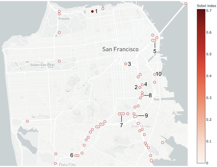
4.7 Accounting for retrofit costs
The proposed method does not allow for an explicit constraint on the total cost of bridge seismic
retrofits as an optimisation problem might (e.g., Gomez & Baker, 2019). By changing the function
whose sensitivity is being analysed, budgetary considerations can be incorporated into an analysis.
To choose a set of retrofits that maximises the reduction in the expected cost of the road network
performance per dollar spent on retrofits, Equation (24) can be used, where CR (f ) denotes the cost
of a set of retrofits described in f .
16Bhattacharjee, G., and Baker, J. W. (2021). “Using global variance-based sensitivity analysis to
prioritise bridge retrofits in a regional road network subject to seismic hazard.” Structure and
Infrastructure Engineering (in press).
Figure 5: Network effects (as given by Equation (23) of bridge retrofits carried out according to six
retrofit prioritisation strategies.
E[C]
Ψ̂(f ) = (24)
CR (f )
To implement Equation (24), it is assumed that retrofitting a bridge costs 25% as much as
repairing it. Figure 6 shows that a strategy based on total-order Sobol’ indices estimated with
respect to Equation (24) outperforms the six other strategies tested. For just 13% of the cost of
retrofitting all 71 bridges, the Sobol’ cost-ratio-based strategy achieves 87.5% of the total reduction
in the network performance cost that can be achieved by retrofitting bridges. That the Sobol’
cost-ratio-based strategy performs so well is not surprising, since none of the other strategies can
take into account the cost of retrofits, a commonly cited limitation of heuristic methods for retrofit
prioritisation. Because the total-order Sobol’ indices with respect to Equation (24) were estimated
using the same set of N = 370 sample evaluations used to prioritise bridges with respect to E[C]
in Sections 4.4 and 4.5, no additional simulations of road network performance were required.
5 Discussion
Implementing Algorithm 1 is straightforward; standard verification problems are well documented,
e.g., estimating the Sobol’ indices of the Ishigami function (Ishigami & Homma, 1990). This section
discusses other practical considerations for using this method: its computational complexity, the
number of samples required, and the effect of the binomial distribution parameter p.
17Bhattacharjee, G., and Baker, J. W. (2021). “Using global variance-based sensitivity analysis to
prioritise bridge retrofits in a regional road network subject to seismic hazard.” Structure and
Infrastructure Engineering (in press).
Figure 6: Reduction in the expected total cost of road network performance, E[C], versus the cost of
retrofitting varying numbers of bridges according to different prioritisation strategies, one of which
is the Sobol’ index strategy based on Equation (24), which accounts for both the road network
performance and the cost of retrofits.
5.1 Computational complexity
Evaluating Ψ̂(fi ) requires sampling damage maps and simulating traffic on each damage map.
Simulating traffic is much more computationally expensive than sampling damage maps. Therefore,
knowing the number of traffic simulations required for a particular number of bridges, nB , number
of ground-motion maps, nS , number of damage maps per ground-motion map, nD , and number
of samples of f , N , is necessary to plan experiments. Equation (25) gives the number of function
evaluations nf required to compute the total-order Sobol’ indices for each bridge in a set of nB
bridges for the function Ψ̂(fi ) ≈ ES [C(f )] using Algorithm 1.
nf = (N × nS × nD )(nB + 1) (25)
Though nf may seem large, the Sobol’ index method is well suited to parallelisation over
samples of f because each sample is evaluated independently. As described in Section 4, if multiple
outputs of interest are stored from each sample evaluation, the same set of samples can be used to
evaluate the sensitivities of each output.
18Bhattacharjee, G., and Baker, J. W. (2021). “Using global variance-based sensitivity analysis to
prioritise bridge retrofits in a regional road network subject to seismic hazard.” Structure and
Infrastructure Engineering (in press).
5.2 Number of samples required
The number of samples required to estimate the Sobol’ indices of a set of bridges is not evident a
priori, in part because the criteria that define a satisfactory estimate vary by application. If the
objective of a study is to develop a probabilistic ranking of bridges to retrofit, then one criterion
might be that the ranking is a confident one, e.g., that the 95% confidence intervals of the bridges’
sensitivity indices do not overlap. This may be difficult to achieve in practice. If the objective of
a study is to select a limited number R of bridges to retrofit, a more achievable criterion might be
that the 95% confidence intervals of the R and R + 1 most influential bridges should not overlap.
Finding an appropriate sample size for an application will likely prove an iterative process and
depend on available computational resources and objective, as it did in the case study, for which 370
samples were used as the basis for the Sobol’ strategy. To investigate the goodness of the ranking
established on the basis of that sample size, in this section 90 additional samples (an increase of
about 25%) are used to estimate bridges’ total-order Sobol’ indices and establish a “final” ranking
against which rankings based on smaller sample sizes can be compared.
Figure 7 shows the convergence of the total-order Sobol’ indices (with respect to E[C]) as a
function of the sample size, N , for the bridges ranked 3rd through 7th most important. Figure 7
was produced using bootstrapping: at each value of N ≤ 460, N samples of the fragility function
parameter vector f that had been previously generated were randomly chosen (with replacement),
on the basis of which bridges’ total-order Sobol’ indices were estimated according to Algorithm 1.
At each N , the aforementioned step was repeated 100 times to estimate the mean, standard devi-
ation, and 95% confidence interval of each bridge’s total-order Sobol’ index. Previous evaluations
of f and associated hybrid points were used.
While the relative importance of the 3rd and 7th most important bridges in Figure 7 is clear
even at N = 10, the 95% confidence intervals of the 4th, 5th, and 6th ranked bridges overlap
even at the maximum N = 460. If our objective were to select R = 4 bridges to retrofit, this
result would be less than ideal. The similarity of the three bridges’ total-order Sobol’ indices
may indicate that selecting any one of them as the fourth retrofit would have a similar effect on
E[C] – however, that cannot be inferred from their total-order indices alone. Let b4 , b5 , and b6
denote the three bridges with similar total-order Sobol’ indices as ranked using N = 460 samples
(i.e., without bootstrapping). To know which bridge would have the greatest effect on EC as the
fourth retrofit, each bridge’s fourth-order sensitivity index with respect to the three bridges already
selected for retrofit would have to be estimated. In lieu of that inconvenient computation, these
three bridges can instead be ranked in decreasing order of their estimated first-order Sobol’ indices
(per Sobol, 1993 and using 370 samples): b6 , b5 , b4 . Because b6 has a larger first-order Sobol’
index than the other two bridges but a similar total-order index, retrofitting b6 fourth would be
expected to reduce E[C] more than retrofitting b4 or b5 . This result is evident in Figure 8, which
shows the performance of Sobol’ index-based retrofit strategies for R ≤ 10 based on sample sizes
of N = 100, 150, 200, 300, 400, and 460. At R = 4, the best-performing strategy chooses b6 , beating
the other strategies by about 1.5%. At R = 5, the best-performing strategies choose b6 , beating the
other strategy by about 2.25%. Whether estimating bridges’ first-order Sobol’ indices is warranted
depends on the objective and the results of the total-order analysis – since the method developed
by Sobol’ for first-order index estimation requires evaluating different hybrid points than those used
to estimate total-order Sobol’ indices, the additional computational expense may be considerable
(Sobol, 1993).
19You can also read