Assessment of Hydrogen Production Costs from Electrolysis: United States and Europe - Author
←
→
Page content transcription
If your browser does not render page correctly, please read the page content below
Assessment of Hydrogen Production Costs from
         Electrolysis: United States and Europe

Author:

A DAM C HRISTENSEN
adam@threeseas.co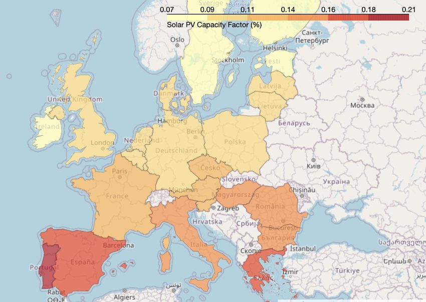
Copyright c 2020

This research was funded by the International Council on Clean Transportation

Final release, June 1, 2020
ii

Contents

1   Executive Summary                                                                                                                                                 1

2   Renewable Hydrogen: Study Outline                                                                                                                                 3
    2.1 Model Scenarios . . . . . . . . . . . . . . . . . . . . . . . . . . . . . . . . . . . . . . . .                                                               4

3   Renewable Generation                                                                                                                                              5
    3.1 Literature Review . . . . . . . . . . . . . . . . . . . . . . . . . . . . . . . . . . . . . . . .                                                             5
    3.2 Overall Economic Modeling Methodology . . . . . . . . . . . . . . . . . . . . . . . . . . .                                                                   7
    3.3 Results – Electricity Prices . . . . . . . . . . . . . . . . . . . . . . . . . . . . . . . . . . .                                                            9

4   Hydrogen Production                                                                                                                                              13
    4.1 Literature Review . . . . . . . . . . . . . . . . . . . .                    .   .   .   .   .   .   .   .   .   .   .   .   .   .   .   .   .   .   .   .   13
    4.2 Electrolyzer CAPEX Costs . . . . . . . . . . . . . . .                       .   .   .   .   .   .   .   .   .   .   .   .   .   .   .   .   .   .   .   .   14
        4.2.1 Comparison of CAPEX Costs to other Studies                             .   .   .   .   .   .   .   .   .   .   .   .   .   .   .   .   .   .   .   .   17
    4.3 Electrolyzer OPEX Costs . . . . . . . . . . . . . . . .                      .   .   .   .   .   .   .   .   .   .   .   .   .   .   .   .   .   .   .   .   18
    4.4 Other System Costs . . . . . . . . . . . . . . . . . . .                     .   .   .   .   .   .   .   .   .   .   .   .   .   .   .   .   .   .   .   .   18
    4.5 Electrolyzer Lifetime . . . . . . . . . . . . . . . . . .                    .   .   .   .   .   .   .   .   .   .   .   .   .   .   .   .   .   .   .   .   19
    4.6 Conversion Efficiency . . . . . . . . . . . . . . . . . .                    .   .   .   .   .   .   .   .   .   .   .   .   .   .   .   .   .   .   .   .   19
    4.7 Overall Economic Modeling Methodology . . . . . . .                          .   .   .   .   .   .   .   .   .   .   .   .   .   .   .   .   .   .   .   .   19

5   Results                                                                                                                                                          21
    5.1 Scenario #1: Results . . . . . . . . . .     .   .   .   .   .   .   .   .   .   .   .   .   .   .   .   .   .   .   .   .   .   .   .   .   .   .   .   .   21
         5.1.1 United States - Hydrogen Prices       .   .   .   .   .   .   .   .   .   .   .   .   .   .   .   .   .   .   .   .   .   .   .   .   .   .   .   .   22
         5.1.2 Europe - Hydrogen Prices . . .        .   .   .   .   .   .   .   .   .   .   .   .   .   .   .   .   .   .   .   .   .   .   .   .   .   .   .   .   26
    5.2 Scenario #2: Results . . . . . . . . . .     .   .   .   .   .   .   .   .   .   .   .   .   .   .   .   .   .   .   .   .   .   .   .   .   .   .   .   .   30
         5.2.1 United States - Hydrogen Prices       .   .   .   .   .   .   .   .   .   .   .   .   .   .   .   .   .   .   .   .   .   .   .   .   .   .   .   .   30
         5.2.2 Europe - Hydrogen Prices . . .        .   .   .   .   .   .   .   .   .   .   .   .   .   .   .   .   .   .   .   .   .   .   .   .   .   .   .   .   34
    5.3 Scenario #3: Results . . . . . . . . . .     .   .   .   .   .   .   .   .   .   .   .   .   .   .   .   .   .   .   .   .   .   .   .   .   .   .   .   .   38
         5.3.1 United States - Hydrogen Prices       .   .   .   .   .   .   .   .   .   .   .   .   .   .   .   .   .   .   .   .   .   .   .   .   .   .   .   .   38
         5.3.2 Europe - Hydrogen Prices . . .        .   .   .   .   .   .   .   .   .   .   .   .   .   .   .   .   .   .   .   .   .   .   .   .   .   .   .   .   42

6   Study Comparison                                                                                                                                                 46
    6.1 Summary of Results from IEA Report . . . .               .   .   .   .   .   .   .   .   .   .   .   .   .   .   .   .   .   .   .   .   .   .   .   .   .   46
         6.1.1 IEA Future of Hydrogen – Figure 12 .              .   .   .   .   .   .   .   .   .   .   .   .   .   .   .   .   .   .   .   .   .   .   .   .   .   46
         6.1.2 IEA Future of Hydrogen – Figure 13 .              .   .   .   .   .   .   .   .   .   .   .   .   .   .   .   .   .   .   .   .   .   .   .   .   .   48
         6.1.3 IEA Future of Hydrogen – Figure 14 .              .   .   .   .   .   .   .   .   .   .   .   .   .   .   .   .   .   .   .   .   .   .   .   .   .   48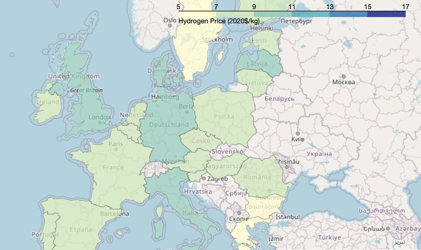
iii

      6.1.4 IEA Future of Hydrogen – Figure 16 . . . . . . . . . . . . . . . . .      .   .   .   .   .   .   .   .   .   49
6.2   Summary of Results from Bloomberg New Energy Finance Report . . . . .           .   .   .   .   .   .   .   .   .   51
      6.2.1 Capital Costs for Chinese Electrolyzers . . . . . . . . . . . . . . .     .   .   .   .   .   .   .   .   .   51
      6.2.2 Modeling Assumptions and Technical Parameters . . . . . . . . . .         .   .   .   .   .   .   .   .   .   51
      6.2.3 H2 Cost – Grid Connected/Continuous Operation . . . . . . . . . .         .   .   .   .   .   .   .   .   .   52
      6.2.4 H2 Cost – Grid Connected/Off-Peak Electricity Prices . . . . . . .        .   .   .   .   .   .   .   .   .   52
      6.2.5 H2 Cost – Grid Connected/Curtailed Electricity . . . . . . . . . . .      .   .   .   .   .   .   .   .   .   52
      6.2.6 H2 Cost – Direct Connection to a Renewable Electricity Generator          .   .   .   .   .   .   .   .   .   53
      6.2.7 Electricity Price Projections . . . . . . . . . . . . . . . . . . . . .   .   .   .   .   .   .   .   .   .   54
      6.2.8 CAPEX Forecasting . . . . . . . . . . . . . . . . . . . . . . . . .       .   .   .   .   .   .   .   .   .   54
6.3   Summary of Results from IRENA Report . . . . . . . . . . . . . . . . . .        .   .   .   .   .   .   .   .   .   55
      6.3.1 IRENA – Figure 9 . . . . . . . . . . . . . . . . . . . . . . . . . .      .   .   .   .   .   .   .   .   .   55
      6.3.2 IRENA – Figure 10 . . . . . . . . . . . . . . . . . . . . . . . . . .     .   .   .   .   .   .   .   .   .   56
      6.3.3 IRENA – Figure 11 . . . . . . . . . . . . . . . . . . . . . . . . . .     .   .   .   .   .   .   .   .   .   57
      6.3.4 IRENA – Figure 14 . . . . . . . . . . . . . . . . . . . . . . . . . .     .   .   .   .   .   .   .   .   .   58
iv
List of Figures
2.1 Model plant for the production of renewable hydrogen. . . . . . . . . . . . . . . . . . . . . 3
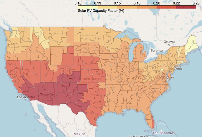
3.1 Capacity factor for solar PV systems in the US. . . . . . . . . . . . . . . . . . . . . . . . . 6
3.2 Capacity factor for onshore wind systems in the US. . . . . . . . . . . . . . . . . . . . . . . 6
3.3 Capacity factor for offshore wind systems in the US. Grey regions indicate that offshore
systems are not feasible. . . . . . . . . . . . . . . . . . . . . . . . . . . . . . . . . . . . . 7
3.4 Capacity factor for solar PV systems in Europe. . . . . . . . . . . . . . . . . . . . . . . . . 8
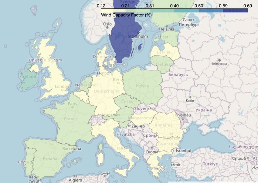
3.5 Capacity factor for both on and offshore wind systems in Europe. . . . . . . . . . . . . . . . 8
3.6 Electricity prices for solar for Scenario #1. The boxplot shows the range in electricity price
that could be expected in the US based on resource availability. . . . . . . . . . . . . . . . . 10
3.7 Electricity prices for onshore wind for Scenario #1. The boxplot shows the range in elec-
tricity price that could be expected in the US based on resource availability. . . . . . . . . . 10
3.8 Electricity prices for offshore wind for Scenario #1. The boxplot shows the range in elec-
tricity price that could be expected in the US based on resource availability. . . . . . . . . . 11
3.9 Electricity prices for solar for Scenario #2. The boxplot shows the range in electricity price
that could be expected in the US based on resource availability. . . . . . . . . . . . . . . . . 11
3.10 Electricity prices for onshore wind for Scenario #2. The boxplot shows the range in elec-
tricity price that could be expected in the US based on resource availability. . . . . . . . . . 12
3.11 Electricity prices for offshore wind for Scenario #2. The boxplot shows the range in elec-
tricity price that could be expected in the US based on resource availability. . . . . . . . . . 12
5.1 H2 prices in 2020 – United States – Scenario #1 (grid connected) . . . . . . . . . . . . . . . 22
5.2 H2 prices in 2025 – United States – Scenario #1 (grid connected) . . . . . . . . . . . . . . . 22
5.3 H2 prices in 2030 – United States – Scenario #1 (grid connected) . . . . . . . . . . . . . . . 23
5.4 H2 prices in 2035 – United States – Scenario #1 (grid connected) . . . . . . . . . . . . . . . 23
5.5 H2 prices in 2040 – United States – Scenario #1 (grid connected) . . . . . . . . . . . . . . . 24
5.6 H2 prices in 2045 – United States – Scenario #1 (grid connected) . . . . . . . . . . . . . . . 24
5.7 H2 prices in 2050 – United States – Scenario #1 (grid connected) . . . . . . . . . . . . . . . 25
5.8 H2 prices in 2020 – Europe – Scenario #1 (grid connected) . . . . . . . . . . . . . . . . . . 26
5.9 H2 prices in 2025 – Europe – Scenario #1 (grid connected) . . . . . . . . . . . . . . . . . . 26
5.10 H2 prices in 2030 – Europe – Scenario #1 (grid connected) . . . . . . . . . . . . . . . . . . 27
5.11 H2 prices in 2035 – Europe – Scenario #1 (grid connected) . . . . . . . . . . . . . . . . . . 27
5.12 H2 prices in 2040 – Europe – Scenario #1 (grid connected) . . . . . . . . . . . . . . . . . . 28
5.13 H2 prices in 2045 – Europe – Scenario #1 (grid connected) . . . . . . . . . . . . . . . . . . 28
5.14 H2 prices in 2050 – Europe – Scenario #1 (grid connected) . . . . . . . . . . . . . . . . . . 29
5.15 H2 prices in 2020 – United States – Scenario #2 (direct connection) . . . . . . . . . . . . . 30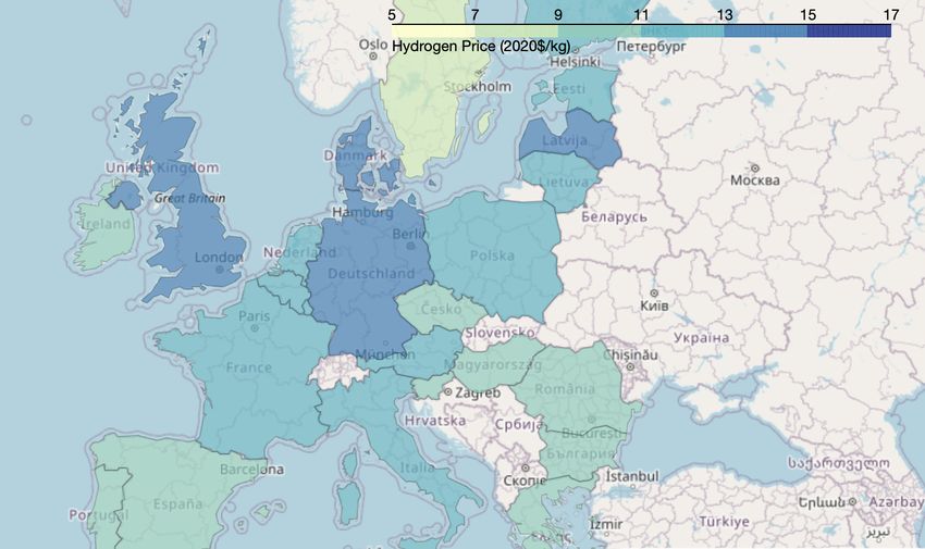
v

5.16   H2 prices in 2025 – United States – Scenario #2 (direct connection) .                                  .   .   .   .   .   .   .   .   .   .   .   .   31
5.17   H2 prices in 2030 – United States – Scenario #2 (direct connection) .                                  .   .   .   .   .   .   .   .   .   .   .   .   31
5.18   H2 prices in 2035 – United States – Scenario #2 (direct connection) .                                  .   .   .   .   .   .   .   .   .   .   .   .   32
5.19   H2 prices in 2040 – United States – Scenario #2 (direct connection) .                                  .   .   .   .   .   .   .   .   .   .   .   .   32
5.20   H2 prices in 2045 – United States – Scenario #2 (direct connection) .                                  .   .   .   .   .   .   .   .   .   .   .   .   33
5.21   H2 prices in 2050 – United States – Scenario #2 (direct connection) .                                  .   .   .   .   .   .   .   .   .   .   .   .   33
5.22   H2 prices in 2020 – Europe – Scenario #2 (direct connection) . . . . .                                 .   .   .   .   .   .   .   .   .   .   .   .   34
5.23   H2 prices in 2025 – Europe – Scenario #2 (direct connection) . . . . .                                 .   .   .   .   .   .   .   .   .   .   .   .   34
5.24   H2 prices in 2030 – Europe – Scenario #2 (direct connection) . . . . .                                 .   .   .   .   .   .   .   .   .   .   .   .   35
5.25   H2 prices in 2035 – Europe – Scenario #2 (direct connection) . . . . .                                 .   .   .   .   .   .   .   .   .   .   .   .   35
5.26   H2 prices in 2040 – Europe – Scenario #2 (direct connection) . . . . .                                 .   .   .   .   .   .   .   .   .   .   .   .   36
5.27   H2 prices in 2045 – Europe – Scenario #2 (direct connection) . . . . .                                 .   .   .   .   .   .   .   .   .   .   .   .   36
5.28   H2 prices in 2050 – Europe – Scenario #2 (direct connection) . . . . .                                 .   .   .   .   .   .   .   .   .   .   .   .   37
5.29   H2 prices in 2020 – United States – Scenario #3 (curtailed electricity)                                .   .   .   .   .   .   .   .   .   .   .   .   38
5.30   H2 prices in 2025 – United States – Scenario #3 (curtailed electricity)                                .   .   .   .   .   .   .   .   .   .   .   .   39
5.31   H2 prices in 2030 – United States – Scenario #3 (curtailed electricity)                                .   .   .   .   .   .   .   .   .   .   .   .   39
5.32   H2 prices in 2035 – United States – Scenario #3 (curtailed electricity)                                .   .   .   .   .   .   .   .   .   .   .   .   40
5.33   H2 prices in 2040 – United States – Scenario #3 (curtailed electricity)                                .   .   .   .   .   .   .   .   .   .   .   .   40
5.34   H2 prices in 2045 – United States – Scenario #3 (curtailed electricity)                                .   .   .   .   .   .   .   .   .   .   .   .   41
5.35   H2 prices in 2050 – United States – Scenario #3 (curtailed electricity)                                .   .   .   .   .   .   .   .   .   .   .   .   41
5.36   H2 prices in 2020 – Europe – Scenario #3 (curtailed electricity) . . .                                 .   .   .   .   .   .   .   .   .   .   .   .   42
5.37   H2 prices in 2025 – Europe – Scenario #3 (curtailed electricity) . . .                                 .   .   .   .   .   .   .   .   .   .   .   .   42
5.38   H2 prices in 2030 – Europe – Scenario #3 (curtailed electricity) . . .                                 .   .   .   .   .   .   .   .   .   .   .   .   43
5.39   H2 prices in 2035 – Europe – Scenario #3 (curtailed electricity) . . .                                 .   .   .   .   .   .   .   .   .   .   .   .   43
5.40   H2 prices in 2040 – Europe – Scenario #3 (curtailed electricity) . . .                                 .   .   .   .   .   .   .   .   .   .   .   .   44
5.41   H2 prices in 2045 – Europe – Scenario #3 (curtailed electricity) . . .                                 .   .   .   .   .   .   .   .   .   .   .   .   44
5.42   H2 prices in 2050 – Europe – Scenario #3 (curtailed electricity) . . .                                 .   .   .   .   .   .   .   .   .   .   .   .   45

6.1    IEA – Figure 12, reproduced from [5] . .   .   .   .   .   .   .   .   .   .   .   .   .   .   .   .   .   .   .   .   .   .   .   .   .   .   .   .   47
6.2    IEA – Figure 13, reproduced from [5] . .   .   .   .   .   .   .   .   .   .   .   .   .   .   .   .   .   .   .   .   .   .   .   .   .   .   .   .   48
6.3    IEA – Figure 14, reproduced from [5] . .   .   .   .   .   .   .   .   .   .   .   .   .   .   .   .   .   .   .   .   .   .   .   .   .   .   .   .   49
6.4    IEA – Figure 16, reproduced from [5] . .   .   .   .   .   .   .   .   .   .   .   .   .   .   .   .   .   .   .   .   .   .   .   .   .   .   .   .   50
6.5    IRENA – Figure 9, reproduced from [7] .    .   .   .   .   .   .   .   .   .   .   .   .   .   .   .   .   .   .   .   .   .   .   .   .   .   .   .   55
6.6    IRENA – Figure 10, reproduced from [7]     .   .   .   .   .   .   .   .   .   .   .   .   .   .   .   .   .   .   .   .   .   .   .   .   .   .   .   56
6.7    IRENA – Figure 11, reproduced from [7]     .   .   .   .   .   .   .   .   .   .   .   .   .   .   .   .   .   .   .   .   .   .   .   .   .   .   .   57
6.8    IRENA – Figure 14, reproduced from [7]     .   .   .   .   .   .   .   .   .   .   .   .   .   .   .   .   .   .   .   .   .   .   .   .   .   .   .   58
vi

List of Tables

 3.1   Parameters used in the levelized cost of energy calculations . . . . . . . . . . . . . . . . . .                                         9

 4.1   Referenced Electrolyzer CAPEX Costs from Glenk et al. .         .   .   .   .   .   .   .   .   .   .   .   .   .   .   .   .   .   .   14
 4.2   Electrolyzer CAPEX price parameters. . . . . . . . . . . .      .   .   .   .   .   .   .   .   .   .   .   .   .   .   .   .   .   .   17
 4.3   Comparison of electrolyzer CAPEX costs to other studies.        .   .   .   .   .   .   .   .   .   .   .   .   .   .   .   .   .   .   18
 4.4   Electrolyzer efficiencies (ηE2H ) used in this study. . . . .   .   .   .   .   .   .   .   .   .   .   .   .   .   .   .   .   .   .   19
 4.5   Fundamental economic parameters for NPV calculations. .         .   .   .   .   .   .   .   .   .   .   .   .   .   .   .   .   .   .   20

 6.1   LCOH Summary from the BNEF Report . . . . . . . . . . . . . . . . . . . . . . . . . . . . 54
 6.2   Comparison of assumptions used in IRENA Figure 11. . . . . . . . . . . . . . . . . . . . . 58
vii

List of Abbreviations

                   AE      Alkaline Electrolyzer
                   BNEF    Bloomberg New Energy Finance
                   EU      European Union
                   IEA     International Energy Agency
                   IRENA   International REnewable Energy Agency
                   kW      kilowatt
                   LCOE    Levelized Cost of Electricity
                   LCOH    Levelized Cost of Hydrogen
                   MW      Megawatt
                   NPV     Net Present Value
                   NREL    National Renewable Energy Laboratory
                   PEM     Proton Exchange Membrane
                   SOE     Solid Oxide Electrolyzer Cell
                   TRB     Technical Resource Bin
                   US      United States
                   WACC    Weighted Average Cost of Capital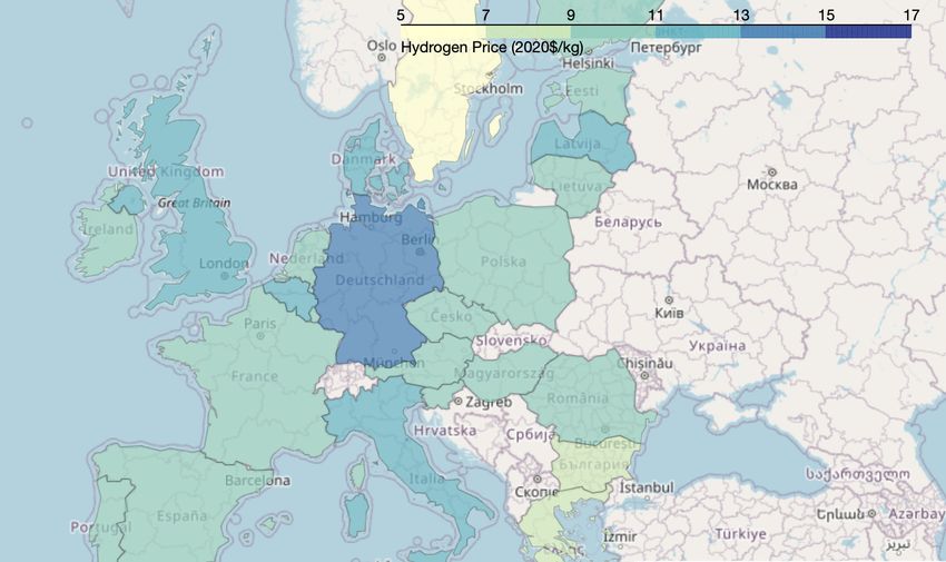
viii

Acknowledgements

This project was generously funded by the the International Council on Clean Transportation.
1

Chapter 1

Executive Summary

This work examines the price of H2 production from renewable electricity generators in both the United
States and the European Union. Many other reports exist on this topic, but with varying degrees of trans-
parency to cost assumptions. These methodological differences make it difficult to compare H2 prices from
different studies without first examining all the details. We note that many high profile studies report H2
prices that ignore other system costs beyond those associated with the electrolyzer CAPEX and the purchase
of electricity to operate the electrolyzer. There are, of course, other system costs that must be considered in
order to build out a fully operational H2 electrolysis plant. Data on these other system costs are still not well
understood and should be documented more fully, but to zero them out completely could be misleading.
We also note that many of the projections of electricity price would be considered optimistic even when
compared to the optimistic electricity price scenarios included in this work. In some cases these “best” case
scenarios might represent a “global best” while other projections of electricity price are more opaque.
     In this study we assume plant costs originate from the electrolyzer CAPEX, electrolyzer replacement
(if necessary), electricity, water, piping, compressor CAPEX, storage, dispensing, and other fixed OPEX
costs. With these data, we attempt to build the most transparent accounting of H2 prices when produced
from a variety of renewable electricity generators. Our data is drawn only from public sources and includes
a large database of CAPEX prices and capacity factors for wind and solar generators for the United States
and Europe. This geographically explicit data is leveraged to calculate the distribution of H2 price for both
the US and EU under three different connection configurations. Scenario #1 assumes that the electrolyzer
is connected to the larger electric grid and can benefit from high capacity factors (but must pay associated
grid fees). Scenario #2 assums that the electrolyzer is directly connected to a renewable electricity generator
(and thus does not need to pay grid fees, but the electrolyzer can only be operated at the capacity factor of
the renewable electricity generator). Scenario #3 assumes that the electrolyzer is only operated on electricity
that would otherwise be curtailed. Our primary results are summarized below; the minimum prices shown
here correspond with the most favorable locations within the EU and US.

    Grid Connected

   • The median price of H2 (in the US, 2020-2050) will decrease from $11.59/kg to $8.44/kg; the mini-
     mum price decreases from $8.80/kg to $6.81/kg.

   • The median price of H2 (in the EU, 2020-2050) will decrease from $16.05/kg to $10.46/kg; the
     minimum price decreases from $7.49/kg to $5.80/kg.

    Direct Connection
Chapter 1. Executive Summary 2
• The median price of H2 (in the US, 2020-2050) will decrease from $13.08/kg to $8.33/kg; the mini-
mum price decreases from $7.12/kg to $4.90/kg.
• The median price of H2 (in the EU, 2020-2050) will decrease from $21.76/kg to $12.46/kg; the
minimum price decreases from $6.62/kg to $4.70/kg.
Curtailed Electricity
• The median price of H2 (in the US, 2020-2050) will decrease from $12.50/kg to $8.15/kg; the mini-
mum price decreases from $8.48/kg to $7.13/kg.
• The median price of H2 (in the EU, 2020-2050) will decrease from $12.97/kg to $8.43/kg; the mini-
mum price decreases from $8.43/kg to $7.13/kg.
The hydrogen price (when produced from renewable electricity generators) calculated here is highly
dependent on geographic location with significantly cheaper production prices in some favorable localities.3
Chapter 2
Renewable Hydrogen: Study Outline
The primary objective of this report is to develop an understanding of the costs associated with the pro-
duction of hydrogen from water electrolysis using various forms of intermittent renewable electricity in the
United States (US) and European Union (EU). Throughout this analysis we do not make any assumptions
regarding policy incentives or other financial benefits. These modeling assumptions, which are often found
in the literature, can obscure the results making it difficult for policy-makers/analysts to compile data and
make recommendations. This analysis covers both the United States (excluding Alaska and Hawaii) and Eu-
rope from the years 2020-2050. A basic block diagram model of a power-to-gas system is shown in Figure
2.1.
F IGURE 2.1: Model plant for the production of renewable hydrogen.
For this study we focus on three renewable electricity technologies: (1) solar photovoltaic (utility scale),
(2) onshore wind, and (3) offshore wind. We assume that there are three primary electrolyzer technologies
that could be interconnected with these renewable electricity generators. The electrolyzer technologies that
are considered in this study are: alkaline electrolyzer (AE), proton exchange membrane (PEM), and solid-
oxide electrolyzers (SOE). The output from each of these electrolyzers will be a concentrated stream of
hydrogen gas as well as oxygen. In the case of the PEM electrolyzer, we assume that the PEM is a “high
pressure” PEM, which negates the need for an external hydrogen compressor – only the AE and SOE will
require a final compression stage.
The hydrogen produced from these reactions must then be captured and transported to demand centers
either though pipelines (that must be built) or tanker truck/train. These post-production steps add additional
costs that are not captured in this work. For purposes of this study, we focus only the costs associated with
capital expenditures and all fixed/variable costs associated with production of hydrogen and compression.
For purposes of modeling these systems it is assumed that any renewable technology could be paired
with any other electrolyzer technology – full enumeration yields nine unique power-to-gas configurations.Chapter 2. Renewable Hydrogen: Study Outline 4
2.1 Model Scenarios
In addition to assuming the nine system configurations we consider three scenarios that attempt to capture
the various ways an electrolyzer could be physically connected to a renewable electricity generator. These
scenarios reflect proposals that have been considered at various levels of government – making them policy
relevant. The three bounding scenarios are:
• Scenario 1 – Grid Connect: We assume that the electrolyzer is grid connected and therefore can pro-
duce hydrogen gas at a 100% capacity factor – the ratio of an actual electrical energy output over
a given period of time to the maximum possible electrical energy output. If the electrolyzer is grid
connected it is assumed that the business would contract either with a utility or directly to electric-
ity generators through long-term power purchase agreements to procure only renewable electricity.
We estimate the electricity price the business would pay as the price of electricity generation plus
transmission and distribution charges.
• Scenario 2 – Direct Connect: We assume that the electrolyzer is independent of the larger transmis-
sion grid and instead is connected directly to a renewable electricity generator. Under this scenario
the price of electricity is lower that in Scenario 1 because transmission and distribution charges are
not considered. However, the intermittency of the renewable electricity generator means that the elec-
trolyzer’s capacity factor is equal to the generator’s capacity factor. We make no assumptions about
co-location, just that all the energy from the renewable electricity generator flows to the electrolyzer
and nowhere else. For simplicity, we do not model any sort of hybrid solar/wind systems in order to
increase the effective capacity factor.
• Scenario 3 – Curtailed Electricity: In this scenario we assume that the electrolyzer is grid connected,
but serves only as a load balancing/storage entity. We assume that in times of high renewable gen-
eration some energy would need to be curtailed at zero $/kWh. We recognize that the number of
hours per day that curtailed energy would be available would vary enormously by location and across
time. Absent a model that can capture the market-based behavior of the transmission grid, we simply
assume a flat 4 hours per day.
The following chapters present a literature review, discussion of the modeling methodology, and presen-
tation of economic parameters used to project renewable hydrogen prices.5
Chapter 3
Renewable Generation
This chapter will review primary sources of data that, ultimately, will instantiate a cash flow economic model
of a renewable electricity generator.
3.1 Literature Review
Uncertainty exists regarding many of the techno-economic parameters that are necessary to construct an
economic model of a renewable electricity generator. Not only must the data for renewable electricity gen-
erators be projected out to 2050, but it must also be free of inconsistencies that might hamper comparisons
between different technology categories being modeled. To that end, the only public data source that is
available for these technology descriptions is the National Renewable Energy Laboratory’s (NREL) Annual
Technology Baseline (ATB) [1]. NREL’s ATB dataset projects various techno-economic parameters out to
2050 along three paths – a pessimistic constant path, a optimistic low and a middle path (mid). Data exists
for a number of technology categories beyond those considered in this work. This database only includes
United States data, however, it is assumed that these data for utility scale solar/wind investments fluctuate
on a global scale, as such, European rates will not differ significantly.
The technical and financial operation of a renewable generation plant can be approximated with a suite
of parameters, which are detailed in Table 3.1 – installed capacity (kW), generator droop (%/yr), inverter
costs ($/kW), inverter lifetime (yr), CAPEX rate ($/kW), wind turbine blade replacement rates, fixed op-
eration/maintenance costs ($/kW), and variable operation/maintenance costs ($/kWh). Capacity factor (%)
is another extremely important modeling parameter that is often used to describe the intermittency of a re-
newable electricity generator. While NREL’s ATB does provide capacity factor projections out to 2050, the
geographical extent of the data is limited to only a couple discrete cities in the US. We supplement the ATB
dataset with capacity factor data from NREL’s Renewable Energy Deployment System (ReEDS) modeling
system [2]. Specifically, we use capacity factor data from the ReEDS modeling system because of the ge-
ographic resolution, but capacity factor improvement over time is not captured natively in this dataset. To
represent this dimension of technological improvement we apply the year-by-year improvement rate from
the ATB dataset to the ReEDS data. These improvement rates are also detailed in Table 3.1. Figures 3.1,
3.2, and 3.3 show the capacity factor used in this analysis.
The raw NREL ReEDS capacity factor data is reported for 356 regions in the US at an hourly timescale
for a number of technical resource bins (TRBs). Technical resource bins help describe the resource potential
(i.e., wind speed, solar insolation, etc.) that is available at a location. We aggregate the ReEDS data toChapter 3. Renewable Generation 6
F IGURE 3.1: Capacity factor for solar PV systems in the US.
F IGURE 3.2: Capacity factor for onshore wind systems in the US.
annual, TRB weighted, capacity factors. This way we have 356 capacity factors for each of our three
renewable electricity generators.
Data of this resolution was not available for Europe, instead we use data generated at the country levelChapter 3. Renewable Generation 7
F IGURE 3.3: Capacity factor for offshore wind systems in the US. Grey regions indicate that
offshore systems are not feasible.
from [3, 4], shown in Figures 3.4 and 3.5. Furthermore, this data was not differentiated by wind technology
type; we assume that both onshore and offshore wind systems have the same capacity factor.
3.2 Overall Economic Modeling Methodology
Electricity price projections were estimated as the time series of Levelized Cost of Energy (LCOE) for wind
and solar systems in Europe from 2020-2050 for the three projection pathways (low, mid, and constant)
that were specified in NREL’s ATB dataset. The LCOE is a measure of the average total cost to build and
operate a generator over its lifetime divided by the total energy output over the lifetime of the plant. In other
words, this measure allows one to calculate the minimum price necessary to sell energy in order to meet a
certain hurdle rate – the hurdle rate is the minimum rate of return on a project or investment. In this study
a hurdle rate of 7% was assumed for both new solar/wind projects; this is consistent with a technology that
has been proven commercial at global scales. The aggregated parameters needed to describe both wind and
solar cash flows are described in Table 3.1. It was assumed that the generator system had zero salvage value
at the end-of-life and that accelerated depreciation (5-year) was calculated with a straight-line method.Chapter 3. Renewable Generation 8
F IGURE 3.4: Capacity factor for solar PV systems in Europe.
F IGURE 3.5: Capacity factor for both on and offshore wind systems in Europe.Chapter 3. Renewable Generation 9
TABLE 3.1: Parameters used in the levelized cost of energy calculations
Data Description Solar Wind
System Life 30 years 30 years
Rate of Capital Expenditure ($kW/DC) [1] [1]
Generator Capacity Factor (%) See 3.1, 3.2, 3.3 See 3.4, 3.5
Fixed Operations and Maintenance Costs [1] [1]
Variable Operations and Maintenance Costs [1] [1]
Solar Capacity Factor Improvement 0.14 %/yr —
Onshore Wind Capacity Factor Improvement — 2.25 %/yr (2020-2030), 0.15 %/yr (2030-2050)
Offshore Wind Capacity Factor Improvement — 0.53 %/yr
Generator Performance Degradation -1 %/year -0.5 %/year
Inverter Replacement Cost 100 $/kW DC —
Inverter Lifetime 10 years —
Gearbox Replacement Cost — 15 % of CAPEX rate
Gearbox Lifetime — 7 years
Blade Replacement Cost — 20 % of CAPEX rate
Blade Lifetime — 15 years
Number of Replacement Blades — 1
Using the LCOE metric as a proxy for the actual generation price represents a balance between com-
pleteness and transparency. Using the LCOE metric assumes that the renewable hydrogen plant is able to
obtain electricity from a new plant installed in that year. In reality, the generation-only electricity price
would be a more complicated function of transmission grid dynamics. However, a transparent model
that considers the details of grid effects is not available. We do not assume any incentives for renewable
electricity generation. Tax rates for each country were taken from the Tax Foundation dataset (https:
//taxfoundation.org/publications/corporate-tax-rates-around-the-world/).
3.3 Results – Electricity Prices
This section presents the final US electricity prices for the three price projection pathways (low, mid, and
constant) that were mapped out in NREL’s ATB dataset. Data for Scenario #1 (generation & transmis-
sion/distribution) prices for the three renewable electricity generators are shown in Figures 3.6, 3.7, and 3.8.
Data for Scenario #2 (generation only) prices for the three renewable electricity generators are shown in
Figures 3.9, 3.10, and 3.11. Projections of the LCOE are similar to those electricity prices reported else-
where, although, as will be pointed out in Chapter 6 there are varying degrees of optimism associated with
each individual report [1, 5, 6, 7].
Electricity prices for the EU are not explicitly printed here because they are duplicative except for their
differing transmission and distribution costs; again, it has been assumed that prices for utility scale renewableChapter 3. Renewable Generation 10
electricity generators fluctuate on a global scale. As such, European results follow similar price trends for
Scenario #1.
F IGURE 3.6: Electricity prices for solar for Scenario #1. The boxplot shows the range in
electricity price that could be expected in the US based on resource availability.
F IGURE 3.7: Electricity prices for onshore wind for Scenario #1. The boxplot shows the
range in electricity price that could be expected in the US based on resource availability.Chapter 3. Renewable Generation 11
F IGURE 3.8: Electricity prices for offshore wind for Scenario #1. The boxplot shows the
range in electricity price that could be expected in the US based on resource availability.
F IGURE 3.9: Electricity prices for solar for Scenario #2. The boxplot shows the range in
electricity price that could be expected in the US based on resource availability.Chapter 3. Renewable Generation 12
F IGURE 3.10: Electricity prices for onshore wind for Scenario #2. The boxplot shows the
range in electricity price that could be expected in the US based on resource availability.
F IGURE 3.11: Electricity prices for offshore wind for Scenario #2. The boxplot shows the
range in electricity price that could be expected in the US based on resource availability.13
Chapter 4
Hydrogen Production
This chapter is dedicated to the economic evaluation of renewable hydrogen pathways and begins with
a literature review. The methodology used to perform this evaluation is then described. The following
subsections will also detail the data that was reviewed and used to instantiate our modeling framework.
Results of the analysis are detailed in Chapter 5 for each of the scenarios described in Chapter 2.
4.1 Literature Review
Academic research for producing hydrogen from electrolysis fuels stretches back to 1977 when Steinberg
et al. discussed synthetic methanol production from CO2 , water and nuclear fusion energy [8, 9, 10].
Since 1977 the state of research has morphed in important ways from materials science research to systems
analysis. While the evolution of the research is important context, the main purpose of this literature review
is focused on the state of knowledge on the costs associated with each of the system components. This
analysis focuses on understanding the following parameters:
• Electrolyzer CAPEX costs (for AE, PEM and SOE systems)
• Electrolyzer OPEX costs
• Compressor CAPEX costs (for supplemental compression of H2 gas)
• Compressor OPEX costs (for supplemental compression of H2 gas)
• Balance of System costs (piping, water, etc.)
• Electrolyzer lifetime (dictates when electrolyzer will need to be replaced)
• Conversion efficiency (how efficiently can water be converted to H2 gas)
Generally speaking, there is wide agreement around the conversion efficiency values for the three elec-
trolyzer types (AE, PEM, and SOE). However, there is huge range of variability for all cost parameters. This
is not surprising for a technology that has not reached full maturity. The following sections will detail these
important parameters.Chapter 4. Hydrogen Production 14
4.2 Electrolyzer CAPEX Costs
Until very recently CAPEX costs associated with the electrolyzer that could be found in the literature were
a grab bag of values representing a range of currencies and constant year $ values – occasionally these
values included other system components as well. This unharmonized data made it nearly impossible to
understand larger industry trends for predicting the cost improvements as the industry matured. Efforts by
Brynolf et al. (2017) and more recently by Glenk et al. (2019) were made to harmonize these important
CAPEX parameters [11, 12]. We follow the literature review by Glenk et al. for its completeness and
transparent methodology. Their review included only original sources of data and excluded literature that
did not provide clear costs estimates or methodologies for producing cost estimates. The cost data from the
sources that remained was then harmonized into 2016 e costs to aid technology comparisons. Glenk et al.
caution that only a few points for SOE systems exist; it was not included in their analysis as a result. We
include SOE systems in this analysis simply for completeness, it should only be taken as illustrative. Table
4.1 is from Glenk et al. but includes original sources for completeness.
TABLE 4.1: Referenced Electrolyzer CAPEX Costs from Glenk et al.
Electrolyzer Type Year of Estimate (2016 e/kW) (2020 $/kW) Original Source
AE 2003 1830 2091 [13]
AE 2004 1131 1293 Report – N/A (See [12])
AE 2004 1131 1293 Report – N/A (See [12])
AE 2005 1120 1280 [14]
AE 2007 2129 2433 [15]
AE 2007 1431 1635 [16]
AE 2007 2345 2680 [17]
AE 2007 1210 1383 [18]
AE 2008 1241 1418 [19]
AE 2009 2154 2462 [20]
AE 2010 960 1097 [21]
AE 2011 941 1075 [22]
AE 2011 1417 1619 Report – N/A (See [12])
AE 2013 1215 1389 [23]
AE 2013 1210 1383 [24]
AE 2013 1215 1389 [25]
AE 2013 1569 1793 [26]
AE 2014 1110 1269 [27]
AE 2014 757 865 [28]
AE 2014 1160 1326 [29]
AE 2014 1009 1153 [30]
AE 2014 1160 1326 [31]
AE 2015 1589 1816 Interview (See [12])
AE 2015 976 1115 Interview (See [12])
Continued on next pageChapter 4. Hydrogen Production 15
Table 4.1 – Continued from previous page
Electrolyzer Type Year of Estimate (2016 e/kW) (2020 $/kW) Original Source
AE 2015 1551 1773 Interview (See [12])
AE 2015 1475 1686 Interview (See [12])
AE 2015 1232 1408 Interview (See [12])
AE 2015 1584 1810 Interview (See [12])
AE 2015 1313 1501 Interview (See [12])
AE 2015 1229 1405 Interview (See [12])
AE 2015 940 1074 Interview (See [12])
AE 2015 831 950 Interview (See [12])
AE 2015 1157 1322 Report – N/A (See [12])
AE 2015 1006 1150 Report – N/A (See [12])
AE 2015 1006 1150 Report – N/A (See [12])
AE 2015 1012 1157 [32]
AE 2015 1408 1609 [33]
AE 2016 800 914 Report – N/A (See [12])
AE 2016 1000 1143 Report – N/A (See [12])
AE 2016 1283 1466 Presentation (See [12])
AE 2016 1200 1371 [34]
AE 2016 1000 1143 [35]
AE 2016 1100 1257 [36]
AE 2016 1112 1271 [37]
AE 2017 800 914 Report – N/A (See [12])
AE 2017 1000 1143 Report – N/A (See [12])
AE 2017 1000 1143 Report – N/A (See [12])
AE 2017 975 1114 Report – N/A (See [12])
AE 2020 948 1083 [38]
AE 2025 932 1065 Report – N/A (See [12])
AE 2030 757 865 [39]
AE 2030 645 737 [40]
PEM 2003 1830 2091 [13]
PEM 2004 1131 1293 Report – N/A (See [12])
PEM 2005 2440 2789 [41]
PEM 2008 1587 1814 [42]
PEM 2008 1241 1418 [19]
PEM 2009 2154 2462 [20]
PEM 2010 2133 2438 [43]
PEM 2010 960 1097 [21]
PEM 2013 1569 1793 [26]
PEM 2013 1135 1297 Report – N/A (See [12])
PEM 2014 3227 3688 [44]
PEM 2014 1110 1269 [27]
Continued on next pageChapter 4. Hydrogen Production 16
Table 4.1 – Continued from previous page
Electrolyzer Type Year of Estimate (2016 e/kW) (2020 $/kW) Original Source
PEM 2014 1160 1326 [29]
PEM 2014 2463 2815 [45]
PEM 2014 1009 1153 [30]
PEM 2014 1160 1326 [31]
PEM 2014 1513 1729 [46]
PEM 2014 1670 1909 Interview (See [12])
PEM 2014 1387 1585 Report – N/A (See [12])
PEM 2014 1210 1383 Report – N/A (See [12])
PEM 2015 3420 3909 [47]
PEM 2015 2816 3218 [48]
PEM 2015 1012 1157 [32]
PEM 2015 1157 1322 Report – N/A (See [12])
PEM 2015 1006 1150 Report – N/A (See [12])
PEM 2015 2575 2943 Report – N/A (See [12])
PEM 2015 1006 1150 Report – N/A (See [12])
PEM 2016 1200 1371 [34]
PEM 2016 1000 1143 [35]
PEM 2016 1100 1257 [36]
PEM 2016 1112 1271 [37]
PEM 2016 1283 1466 Presentation (See [12])
PEM 2016 1000 1143 Report – N/A (See [12])
PEM 2017 800 914 Report – N/A (See [12])
PEM 2017 1550 1771 Report – N/A (See [12])
PEM 2017 1000 1143 Report – N/A (See [12])
PEM 2017 975 1114 Report – N/A (See [12])
PEM 2025 932 1065 Report – N/A (See [12])
PEM 2030 645 737 [40]
PEM 2030 1177 1345 [49]
SOE 2012 2172 2482 [50]
SOE 2012 12000 13714 Report – N/A (See [12])
SOE 2015 7500 8571 Report – N/A (See [12])
SOE 2017 4500 5143 Report – N/A (See [12])
SOE 2018 2017 2305 Report – N/A (See [12])
SOE 2020 941 1075 [51]
SOE 2020 593 678 [33]
SOE 2020 2000 2286 Report – N/A (See [12])
SOE 2025 1006 1150 [46]
SOE 2025 925 1057 Report – N/A (See [12])
SOE 2030 1000 1143 [35]
SOE 2030 645 737 [40]
Continued on next pageChapter 4. Hydrogen Production 17
Table 4.1 – Continued from previous page
Electrolyzer Type Year of Estimate (2016 e/kW) (2020 $/kW) Original Source
SOE 2030 354 405 [51]
SOE 2030 1177 1345 [49]
SOE 2030 725 829 Report – N/A (See [12])
SOE 2030 656 750 Report – N/A (See [12])
The result of all this data is that Glenk et al. were able to analyze the trends in electrolyzer annual cost
reductions, although the estimates for cost improvements still reflect the wide range of possible electrolyzer
prices. For PEM systems Glenk et al. suggest that a 4.77 +/- 1.88% per year cost reduction would be
possible, while 2.96 +/- 1.23% per year decline would be possible for AE systems [12]. For this work we
did not attempt to formulate the best measure of central tendency, but instead we adopted a monte carlo-
style approach to analyzing these renewable hydrogen systems. We formulate a low, mid, and high price
projection for AE, PEM and SOE systems that corresponds to the min, mean and max of the cost parameters
(year 2020) from table 4.1. The rate of cost improvements shown in Table 4.2 were chosen to fall within the
range of values for PEM and AE systems from Glenk et al.
TABLE 4.2: Electrolyzer CAPEX price parameters.
System Type Scenario (2020 $/kW) Rate of Improvement (%/yr)
AE low 571 0.5
AE mid 988 2.0
AE high 1268 2.5
PEM low 385 0.5
PEM mid 1182 2.0
PEM high 2068 2.5
SOE low 677 0.5
SOE mid 1346 2.0
SOE high 2285 2.5
4.2.1 Comparison of CAPEX Costs to other Studies
We view the references in Table 4.1 as primary cost references, but there are other policy oriented reports
that have also investigated various aspects of renewable hydrogen production, and thus, rely on their own
estimates of electrolyzer CAPEX costs. Table 4.3 details electrolyzer CAPEX assumptions in various reports
for comparison with ours.Chapter 4. Hydrogen Production 18
TABLE 4.3: Comparison of electrolyzer CAPEX costs to other studies.
Report Electrolyzer Type Year of Estimate (2020 $/kW) This Work (2020 $/kW) Reference
IEA AE 2020 500 571-1268 [5]
IEA AE 2030 400 541-1208 [5]
IEA AE Long Term 200 487-1090 [5]
IRENA AE 2020 840 571-1268 [7]
IRENA AE 2050 200 487-1090 [7]
Bloomberg AE 2019 1200 571-1268 [6]
Bloomberg AE 2022 600-1100 565-1256 [6]
Bloomberg AE 2025 400-1000 556-1238 [6]
Bloomberg AE 2030 115-135 541-1208 [6]
Bloomberg AE 2050 80-98 487-1090 [6]
IEA PEM 2020 1100 385-2068 [5]
IEA PEM 2030 650 365-1968 [5]
IEA PEM Long Term 200 325-1781 [5]
Bloomberg PEM 2019 1400 385-2068 [6]
Bloomberg PEM 2030 425-1000 365-1968 [6]
Bloomberg PEM 2050 150-200 325-1781 [6]
IEA SOE 2020 2800 677-2285 [5]
IEA SOE 2030 800 647-2175 [5]
IEA SOE Long Term 500 587-1968 [5]
4.3 Electrolyzer OPEX Costs
Electrolyzer OPEX costs are most commonly modeled as a fraction of the original CAPEX and have been
previously modeled as independent of the electrolyzer type [11]. Most studies put this value between 1-3%
of the electrolyzer CAPEX [11]. We follow the modeling methodology in Glenk et al. and adopt a fixed
OPEX cost of $40/kW for the US and $50/kW in the EU [12]. Variable OPEX costs associated with the
electrolyzer include the costs of electricity (as modeled), and water (0.08 $/kg of H2 ) [12].
4.4 Other System Costs
In addition to the electrolyzer a renewable hydrogen system will require a compressor and piping in order
to get it ready to be injected into a pipeline or to be put into tanker trucks and shipped; we do not model
the cost of distributing hydrogen to end users. The additional CAPEX costs associated with compression,
storage, dispensing, cooling, and “other costs” for AE and SOEC systems were modeled as a flat 2.97 $/kg of
produced H2 as in Parks et al. [52]. It is assumed that the PEM system would be capable of operating at high
pressures, and thus, an additional compression step is unnecessary. However, the PEM system would still
incur costs associated with storage, dispensing, cooling and “other costs”; these system costs are modeledChapter 4. Hydrogen Production 19
as a flat 1.07 $/kg of produced H2 , again, following Parks et al. [52]. Electricity consumption associated
with the compression system is assumed to be at the rate of 4 kWh/kg of H2 and is charged as the same
electricity price as the electrolyzer. We follow the costs provided in Glenk et al. and apply an additional 50
$/kW for CAPEX costs associated with the balance of system (piping, electrical, etc.).
4.5 Electrolyzer Lifetime
While there is some variability in the reported electolyzer lifetime, there is general agreement that current
AE and PEM systems would have lifetimes of 75,000 and 60,000 hours respectively [5]. We project these
lifetimes out to 2050 with a simple linear relationship up to 125,000 hours [5]. We also follow the Interna-
tional Energy Agency’s estimates of SOE lifetimes: 20,000 hours for current systems out to 87,5000 hours
in 2050 [5]. Following Brynolf et al., once a electrolyzer requires replacement, those replacement costs are
estimated to be 50% of the initial capital costs [11].
4.6 Conversion Efficiency
If a electrolyzer could be built that was 100% efficient it would be able to produce 0.03 kg H2 /kWh. This
ideal is scaled down by a conversion efficiency parameter, which varies by electrolyzer type. Modest im-
provements over time are assumed to follow a linear path out to 2050; Table 4.4 details these parameters.
TABLE 4.4: Electrolyzer efficiencies (ηE2H ) used in this study.
Parameter 2020 Value 2050 Value Reference
AE 70% 80% [5]
PEM 60% 74% [5]
SOE 81% 90% [5]
4.7 Overall Economic Modeling Methodology
In order to calculate the price of hydrogen we develop an economic model that is analogous to that developed
in Section 3.2 – the Levelized Cost of Hydrogen is assumed to be a proxy measure for future market prices
of hydrogen. In this study a hurdle rate of 8% was assumed for the hydrogen project, a value that might
be viewed as more consistent with mature technologies that have already been proven at commercial scales.
While this is not strictly true, AE and PEM systems have been in the marketplace for a long time and are
not necessarily considered a new technology. SOE systems are only now entering the market, and might
command a higher hurdle rate in order to incentivize investments [53]. All this considered, we decided to
choose a bounding value for the hurdle rate rather than over-specify data that cannot be directly supported
from literature.Chapter 4. Hydrogen Production 20
This work considers a range of cash flows that would impact the overall viability of a renewable hydro-
gen plant. These cash flows include: capital expenses, operations and maintenance, electrolyzer replace-
ments, corporate taxes (rates are country specific), depreciation, and feedstock costs (i.e., electricity).
This study performs the economic analysis from the perspective of a project developer (i.e., a company
or companies that wish to build a renewable hydrogen plant in EU or the US). The plant being considered
is assumed to have a 30 year lifetime and is built over a period of 2 years. Table 4.5 details the necessary
economic parameters used in the calculation of the price of hydrogen.
TABLE 4.5: Fundamental economic parameters for NPV calculations.
Parameter Value
Plant Lifetime 30 years (no salvage value)
Construction Time 2 years (75% initial capital in year 1, 25% in year 2)
Depreciation Method Straight Line
Depreciation Rate 5%21
Chapter 5
Results
The economic model that was described in Section 4.7 is now used to generate data for the price of hydrogen
in a Monte Carlo style analysis. This way we can assess the distribution of prices for both the United
States and Europe. Unlike a true Monte Carlo analysis, we do not draw parameters randomly, we simply
enumerate a large number of plausible system configurations. For the United States we have (356 regions) x
(3 electrical generators) x (3 electrical generation scenarios) x (3 electrolyzer technologies) x (3 electrolyzer
scenarios) x (7 scenario years) = 201,852 system configurations; for Europe we have 14,175 possible system
configurations.
The histograms in the following figures show the distribution of plausible H2 price across all possible
regions, renewable electricity generators, and electrolyzer types. The y-axis in this graph is simply the
number of system configurations that fall within the H2 price bins that are shown on the x-axis. The coloring
scheme is meant to draw the eye to the median H2 price, which is an important measure of central tendency.
It is also important to highlight the minimum H2 price; both values are explicitly stated in the text insets.
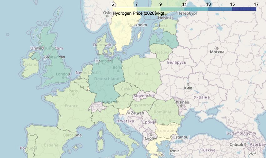
The maps show the geographical distribution of the minimum hydrogen price that can be found for each
time period over all system configurations.
5.1 Scenario #1: Results
Recall that Scenario #1 assumes that the power-to-gas plant is directly connected to the electric grid and
therefore can run at 100% capacity but must pay additional electricity costs associated with transmission
and distribution. The results can be summarized as:
• The median price of H2 in the US will decrease from $11.59/kg in 2020 to $8.44/kg in 2050; during
that same timeframe the minimum price decreases from $8.80/kg to $6.81/kg.
• The median price of H2 in the EU will decrease from $16.05/kg in 2020 to $10.46/kg in 2050; during
that same timeframe the minimum price decreases from $7.49/kg to $5.80/kg.
The following figures show the H2 price distribution and the geographical distribution of the resulting
H2 prices. To clarify futher, the left histogram shows the H2 price distribution across all 201,852 possible
configuration for the US and 14,175 possible configurations for the EU. The H2 price distributions are non-
normal, thus only the median and min values are reported. The data mapped in the right hand side shows
only the minimum price (from any system configuration) for hydrogen that would be available in a specific
region. Regional differences are driven primarily by variation in the potential for renewable electricityChapter 5. Results 22
generation (capacity factor), but corporate tax rates also vary by countries in the EU (it is assumed that all
US regions are subject to a constant composite rate that approximates both state and federal taxes).
Figures 5.1-5.7 summarize the results for the United States between 2020-2050. Figures 5.8-5.14 sum-
marize the results for the European Union between 2020-2050.
5.1.1 United States - Hydrogen Prices
( A ) Distribution of H2 prices over all systems ( B ) Min H2 price found over all system configurations
F IGURE 5.1: H2 prices in 2020 – United States – Scenario #1 (grid connected)
( A ) Distribution of H2 prices over all systems ( B ) Min H2 price found over all system configurations
F IGURE 5.2: H2 prices in 2025 – United States – Scenario #1 (grid connected)Chapter 5. Results 23
( A ) Distribution of H2 prices over all systems ( B ) Min H2 price found over all system configurations
F IGURE 5.3: H2 prices in 2030 – United States – Scenario #1 (grid connected)
( A ) Distribution of H2 prices over all systems ( B ) Min H2 price found over all system configurations
F IGURE 5.4: H2 prices in 2035 – United States – Scenario #1 (grid connected)Chapter 5. Results 24
( A ) Distribution of H2 prices over all systems ( B ) Min H2 price found over all system configurations
F IGURE 5.5: H2 prices in 2040 – United States – Scenario #1 (grid connected)
( A ) Distribution of H2 prices over all systems ( B ) Min H2 price found over all system configurations
F IGURE 5.6: H2 prices in 2045 – United States – Scenario #1 (grid connected)Chapter 5. Results 25
( A ) Distribution of H2 prices over all systems ( B ) Min H2 price found over all system configurations
F IGURE 5.7: H2 prices in 2050 – United States – Scenario #1 (grid connected)Chapter 5. Results 26
5.1.2 Europe - Hydrogen Prices
( A ) Distribution of H2 prices over all systems ( B ) Min H2 price found over all system configurations
F IGURE 5.8: H2 prices in 2020 – Europe – Scenario #1 (grid connected)
( A ) Distribution of H2 prices over all systems ( B ) Min H2 price found over all system configurations
F IGURE 5.9: H2 prices in 2025 – Europe – Scenario #1 (grid connected)Chapter 5. Results 27
( A ) Distribution of H2 prices over all systems ( B ) Min H2 price found over all system configurations
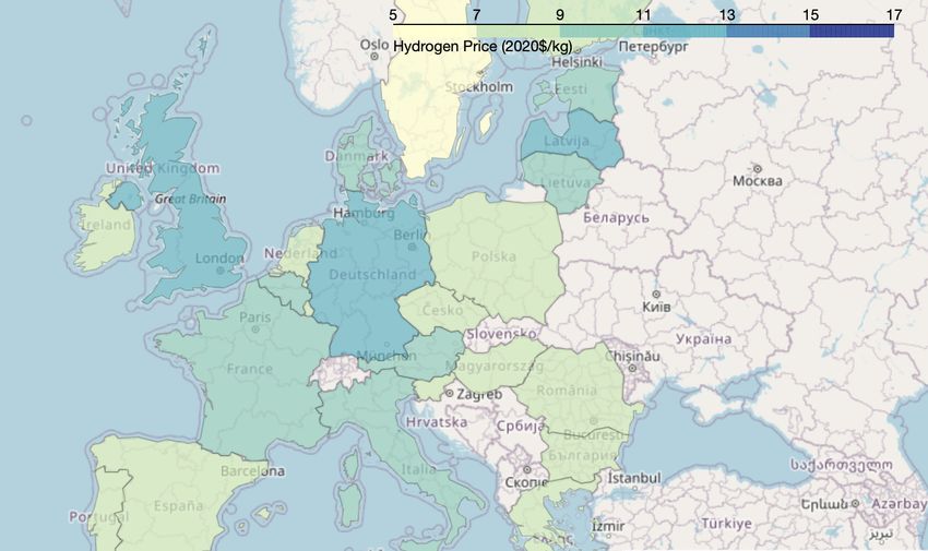
F IGURE 5.10: H2 prices in 2030 – Europe – Scenario #1 (grid connected)
( A ) Distribution of H2 prices over all systems ( B ) Min H2 price found over all system configurations
F IGURE 5.11: H2 prices in 2035 – Europe – Scenario #1 (grid connected)Chapter 5. Results 28
( A ) Distribution of H2 prices over all systems ( B ) Min H2 price found over all system configurations
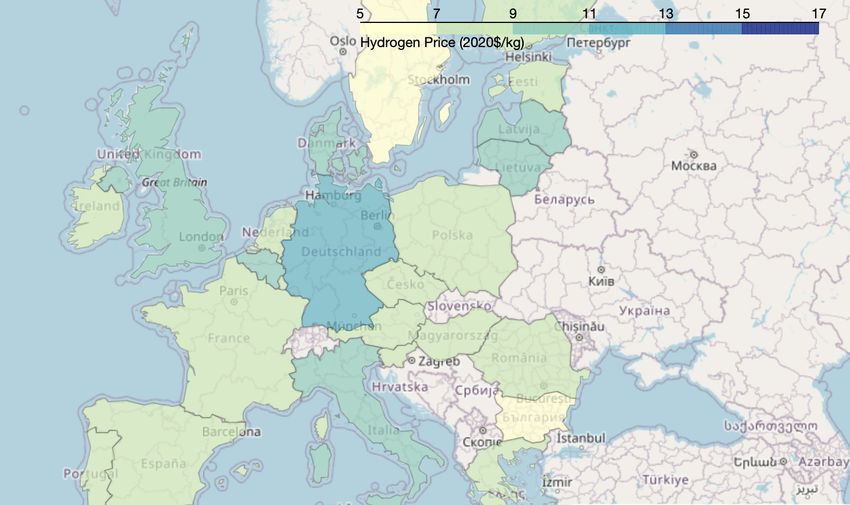
F IGURE 5.12: H2 prices in 2040 – Europe – Scenario #1 (grid connected)
( A ) Distribution of H2 prices over all systems ( B ) Min H2 price found over all system configurations
F IGURE 5.13: H2 prices in 2045 – Europe – Scenario #1 (grid connected)Chapter 5. Results 29
( A ) Distribution of H2 prices over all systems ( B ) Min H2 price found over all system configurations
F IGURE 5.14: H2 prices in 2050 – Europe – Scenario #1 (grid connected)Chapter 5. Results 30
5.2 Scenario #2: Results
Recall that Scenario #2 assumes that the power-to-gas plant is connected to the renewable electricity gener-
ator and therefore will run at the capacity factor of the generator but does not pay electricity costs associated
with transmission and distribution. The results can be summarized as:
• The median price of H2 in the US will decrease from $13.08/kg in 2020 to $8.33/kg in 2050; during
that same timeframe the minimum price decreases from $7.13/kg to $4.90/kg.
• The median price of H2 in the EU will decrease from $21.76/kg in 2020 to $12.46/kg in 2050; during
that same timeframe the minimum price decreases from $6.62/kg to $4.70/kg.
The following figures show the H2 price distribution and the geographical distribution of these H2 prices
(and follow the same analytical logic discussed in section 5.1).
Figures 5.15-5.21 summarize the results for the United States between 2020-2050. Figures 5.22-5.28
summarize the results for the European Union between 2020-2050.
5.2.1 United States - Hydrogen Prices
( A ) Distribution of H2 prices over all systems ( B ) Min H2 price found over all system configurations
F IGURE 5.15: H2 prices in 2020 – United States – Scenario #2 (direct connection)Chapter 5. Results 31
( A ) Distribution of H2 prices over all systems ( B ) Min H2 price found over all system configurations
F IGURE 5.16: H2 prices in 2025 – United States – Scenario #2 (direct connection)
( A ) Distribution of H2 prices over all systems ( B ) Min H2 price found over all system configurations
F IGURE 5.17: H2 prices in 2030 – United States – Scenario #2 (direct connection)Chapter 5. Results 32
( A ) Distribution of H2 prices over all systems ( B ) Min H2 price found over all system configurations
F IGURE 5.18: H2 prices in 2035 – United States – Scenario #2 (direct connection)
( A ) Distribution of H2 prices over all systems ( B ) Min H2 price found over all system configurations
F IGURE 5.19: H2 prices in 2040 – United States – Scenario #2 (direct connection)Chapter 5. Results 33
( A ) Distribution of H2 prices over all systems ( B ) Min H2 price found over all system configurations
F IGURE 5.20: H2 prices in 2045 – United States – Scenario #2 (direct connection)
( A ) Distribution of H2 prices over all systems ( B ) Min H2 price found over all system configurations
F IGURE 5.21: H2 prices in 2050 – United States – Scenario #2 (direct connection)Chapter 5. Results 34
5.2.2 Europe - Hydrogen Prices
( A ) Distribution of H2 prices over all systems ( B ) Min H2 price found over all system configurations
F IGURE 5.22: H2 prices in 2020 – Europe – Scenario #2 (direct connection)
( A ) Distribution of H2 prices over all systems ( B ) Min H2 price found over all system configurations
F IGURE 5.23: H2 prices in 2025 – Europe – Scenario #2 (direct connection)Chapter 5. Results 35
( A ) Distribution of H2 prices over all systems ( B ) Min H2 price found over all system configurations
F IGURE 5.24: H2 prices in 2030 – Europe – Scenario #2 (direct connection)
( A ) Distribution of H2 prices over all systems ( B ) Min H2 price found over all system configurations
F IGURE 5.25: H2 prices in 2035 – Europe – Scenario #2 (direct connection)Chapter 5. Results 36
( A ) Distribution of H2 prices over all systems ( B ) Min H2 price found over all system configurations
F IGURE 5.26: H2 prices in 2040 – Europe – Scenario #2 (direct connection)
( A ) Distribution of H2 prices over all systems ( B ) Min H2 price found over all system configurations
F IGURE 5.27: H2 prices in 2045 – Europe – Scenario #2 (direct connection)Chapter 5. Results 37
( A ) Distribution of H2 prices over all systems ( B ) Min H2 price found over all system configurations
F IGURE 5.28: H2 prices in 2050 – Europe – Scenario #2 (direct connection)Chapter 5. Results 38
5.3 Scenario #3: Results
Recall that Scenario #3 assumes that the power-to-gas plant is connected to the transmission grid, but only
draws energy when renewable energy must be curtailed (assumed to be 4 hours per day = 16% capacity
factor). The curtailed electricity is considered to be free ($0/kWh). The histograms do not show as wide
a distribution as a result of the capacity factor being equalized across all regions – variation is only due to
differences in technology configurations and tax rates. The results can be summarized as:
• The median price of H2 in the US will decrease from $12.50/kg in 2020 to $8.15/kg in 2050; during
that same timeframe the minimum price decreases from $8.48/kg to $7.13/kg.
• The median price of H2 in the EU will decrease from $12.97/kg in 2020 to $8.43/kg in 2050; during
that same timeframe the minimum price decreases from $8.43/kg to $7.13/kg.
5.3.1 United States - Hydrogen Prices
F IGURE 5.29: H2 prices in 2020 – United States – Scenario #3 (curtailed electricity)Chapter 5. Results 39
F IGURE 5.30: H2 prices in 2025 – United States – Scenario #3 (curtailed electricity)
F IGURE 5.31: H2 prices in 2030 – United States – Scenario #3 (curtailed electricity)Chapter 5. Results 40
F IGURE 5.32: H2 prices in 2035 – United States – Scenario #3 (curtailed electricity)
F IGURE 5.33: H2 prices in 2040 – United States – Scenario #3 (curtailed electricity)Chapter 5. Results 41
F IGURE 5.34: H2 prices in 2045 – United States – Scenario #3 (curtailed electricity)
F IGURE 5.35: H2 prices in 2050 – United States – Scenario #3 (curtailed electricity)Chapter 5. Results 42
5.3.2 Europe - Hydrogen Prices
F IGURE 5.36: H2 prices in 2020 – Europe – Scenario #3 (curtailed electricity)
F IGURE 5.37: H2 prices in 2025 – Europe – Scenario #3 (curtailed electricity)Chapter 5. Results 43
F IGURE 5.38: H2 prices in 2030 – Europe – Scenario #3 (curtailed electricity)
F IGURE 5.39: H2 prices in 2035 – Europe – Scenario #3 (curtailed electricity)Chapter 5. Results 44
F IGURE 5.40: H2 prices in 2040 – Europe – Scenario #3 (curtailed electricity)
F IGURE 5.41: H2 prices in 2045 – Europe – Scenario #3 (curtailed electricity)Chapter 5. Results 45
F IGURE 5.42: H2 prices in 2050 – Europe – Scenario #3 (curtailed electricity)46
Chapter 6
Study Comparison
There are a number of economic parameters that are needed in order to fully define the technical and eco-
nomic performance of a power-to-gas system; these parameters are detailed in Chapter 5. Parameter value
differences will result in discrepancies when directly comparing studies, however, it is also important to doc-
ument the underlying set of assumptions that each study uses in order to more fairly compare results. This
chapter is dedicated to documenting the set of assumptions used by three prominent studies by the Inter-
national Energy Agency (IEA), Bloomberg New Energy Finance (BNEF), and the International Renewable
Energy Agency (IRENA) [5, 6, 7].
6.1 Summary of Results from IEA Report
The main results from the IEA that are of concern to this work are summarized in four Figures: 12, 13, 14,
and 16. We will take each of these figures in turn and describe their results and compare them to assumptions
made in this work.
In sum, the IEA report ignores important system costs that are associated with building out a fully
operational H2 electrolysis plant, at the same time their electricity price projections are more optimistic
than even the most optimistic scenario produced by NREL in the Annual Technology Baseline.
6.1.1 IEA Future of Hydrogen – Figure 12Chapter 6. Study Comparison 47
F IGURE 6.1: IEA – Figure 12, reproduced from [5]
Figure 12 is captioned “Future levelised cost of hydrogen (LCOH) production by operating hour for
different electrolyser investment costs (left) and electricity costs (right)” and shows the H2 ($/kg) sensitivity
to different capacity factors (0.0-0.91), electrolyzer CAPEX costs ($250-650/kW), and electricity prices (0-
100 MWh). These graphs were produced under an 8% hurdle rate assumption and an electrolyzer efficiency
of 69%. It is unclear what year these H2 production prices are supposed to represent. It is up to the reader
to infer from the Assumption Annex and Table 3 (page 44-45) that the sensitivity values probably represent
a “Long Term” view of H2 production costs under an optimistic cost reduction scenario.
There is also no discussion of the assumed source of electricity that could provide the range of prices
that IEA includes in this sensitivity test. In this work, we do project electricity prices to be as low as
≈ $0.03/kWh from onshore wind generators, but the capacity factor would be limited to 0.69 (6044 hours)
– this example correspondes to Swedish wind resources. Capacity factors shown in Figure 12 above this
range would require grid connections and therefore would likely need to pay transmission and distribution
charges. These charges, without considering the cost of actually producing the renewable electricity, would
be enough to push the electricity price toward the maximum values that were considered by IEA.
There is little discussion of the methodologies used to project the CAPEX costs, although IEA does
state that “Parameters for the cost and performance of technologies have been based on extensive literature
analysis, conversations with experts and peer review.” The present study uses historical cost trend to project
CAPEX costs out to 2050 (with uncertainty). IEA uses CAPEX values for AE systems that range between
500 $/kW (in 2020) to 200 $/kW in 2050; the present study builds scenarios that use CAPEX values between
571-1268 $/kW in 2020 and 487-1090 $/kW in 2050. More details on other systems can be found in Table
4.3.
While these graphs present the “production” costs, it is up to the reader to interpret exactly what is
meant by “production”. We were able to reproduce the IEA data shown in Figure 12 with our financial
model framework and incorporating the IEA assumptions, but only if we neglected all system costs beyond
the electricity and electrolyzer CAPEX costs. This is in contrast to this work, which only presents H2 pricesYou can also read