Working Paper Series Do macroprudential measures increase inequality? Evidence from the euro area household survey
←
→
Page content transcription
If your browser does not render page correctly, please read the page content below

Working Paper Series
     Oana-Maria Georgescu, Diego Vila Martin    Do macroprudential measures
                                                increase inequality?
                                                Evidence from the euro area
                                                household survey

                                                   No 2567 / June 2021

Disclaimer: This paper should not be reported as representing the views of the European Central Bank
(ECB). The views expressed are those of the authors and do not necessarily reflect those of the ECB.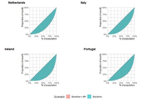
Abstract

          Borrower-based macroprudential (MP) policies - such as caps on loan-to-value (LTV)
      ratios and debt-service-to-income (DSTI) limits - contain the build-up of systemic risk by
      reducing the probability and conditional impact of a crisis. While LTV/DSTI limits can
      increase inequality at introduction, they can dampen the increase in inequality under adverse
      macroeconomic conditions. The relative size of these opposing effects is an empirical question.
      We conduct counterfactual simulations under different macroeconomic and macroprudential
      policy scenarios using granular income and wealth data from the Households Finance and
      Consumption Survey (HFCS) for Ireland, Italy, Netherlands and Portugal. Simulation results
      show that borrower-based measures have a moderate negative welfare impact in terms of
      wealth inequality and a negligible impact on income inequality.

JEL classification: G21, G28, G51.

Keywords: macroprudential policy, inequality, household debt.

ECB Working Paper Series No 2567 / June 2021                                                            1
Non-technical Summary

This paper aims to asses the welfare costs and benefits of borrower-based measures in terms of
wealth and income inequality. Welfare costs arise if wealth and potentially income inequality
increase after the imposition of LTV and DSTI limits compared to the counterfactual without
these limits. The benefits of borrower-based measures may occur as a result of a lower probability
and conditional impact of a financial crisis. Since unemployment in a recession is higher for low
income borrowers, an adverse macroeconomic scenario with borrower-based measure in place
may result in a lower increase in income inequality compared to the counterfactual adverse
scenario without LTV and DSTI limits in place.

To quantify the size of these costs and benefits, we conduct counterfactual simulations comparing
wealth and income inequality under 4 policy scenarios (baseline and adverse scenario, with and
without borrower-based measures in place). The paper restricts the scope of the study to four
euro area countries: Ireland, Italy, Netherlands and Portugal.

To estimate the benefits of macroprudential measures, we proceed in three steps. First, we use a
Bayesian VAR (BVAR) to quantify the macroeconomic impact of a credit crunch conditional on
an adverse macroeconomic scenario under different macroprudential policy regimes (i.e. with or
without LTV and DSTI limits). In a second step, we match the unemployment and asset price
response obtained in the BVAR to household data in order to derive income and wealth distri-
butions under these different policy scenarios. Last, we compute the benefit as the difference
in income (wealth) inequality between the adverse scenario without borrower-based macropru-
dential measures compared to the adverse scenario with these measures in place. The cost is
computed in a similar fashion, as the difference in income and wealth inequality between the
baseline scenarios with and without the borrower-based measures in place. The only difference
to the benefits calculation is that the macroeconomic response is computed conditional on a
loan demand shock following the implementation of borrower-based measures.

We use the Gini coefficient of wealth and income as a metric for our cost-benefit calculations.
We derive the unconditional net benefit as the difference between the expected values of the
Gini coefficient with and without borrower-based measures, taking into account the change in
the crisis probability across policy scenarios.

In terms of wealth inequality, the unconditional benefit is negative, ranging from -0.14 percentage
points in Italy to -0.58 percentage points in the Netherlands. The negative unconditional benefit
implies a net increase in wealth inequality relative to the counterfactual without borrower-based
measures. In the case of income inequality, the unconditional benefit of borrower-based measures
is marginally positive, ranging from 0.04 percentage points for Italy to 0.16 percentage points
for Ireland. These results suggest that the welfare cost of macroprudential regulation in terms
of wealth inequality is contained, while the benefit in terms of income inequality is negligible.

ECB Working Paper Series No 2567 / June 2021                                                        2
1    Introduction

In many advanced economies, home ownership is part of the social contract between policy
makers and citizens, acting as a symbol for social inclusion and economic growth. In this
sense, the housing finance deregulation in the decade preceding the Great Financial Crisis in
the US and UK was meant to act as a redistributive force, potentially reducing wealth and
income inequality (Arundel and Ronald (2020), Rajan (2011), p. 35-40). After the bursting
of the sub-prime housing bubble in 2008, access to mortgage loans has been tightened in most
euro area countries. In this context, macroprudential policies (MP) have been widely used by
policy makers due to their ability to address the build-up of asset price bubbles and excessive
risk-taking by banks. Some of these measures can target banks, for example countercyclical
capital requirements, while others target borrowers, such as the loan-to-value ratio (LTV) or the
debt-service-to-income limit (DSTI).1

While the main policy objective of MP is to enhance financial stability by increasing the resilience
of banks, some studies pointed to the potential negative welfare effects of these policies in terms
of wealth and income inequality (Frost and Stralen (2018); Carpantier et al. (2016)). In good
times, LTV and DSTI limits may have direct redistributive effects by excluding low income
households from the mortgage market. In bad times, macroprudential policy may dampen
the increase in inequality by smoothing the credit cycle, thus lowering the probability and the
conditional impact of a financial crisis. The relative size of these opposing effects is an empirical
question.

To quantify the size of these costs and benefits, we conduct counterfactual simulations comparing
wealth and income inequality under four policy scenarios (baseline and adverse scenario, with
and without MP) for four euro area countries: Ireland, Italy, Netherlands and Portugal. The
analysis combines granular household level data on wealth and income from the Euro Area
Household Finance and Consumption Survey (HFCS) together with bank level data from the
2018 Euro Area Stress Test exercise and macroeconomic indicators from the ECB Statistical
Data Warehouse.2 We use the Gini coefficient as a metric for our cost-benefit calculations.

To estimate the benefits of macroprudential measures, we proceed in three steps. First, we use
a Bayesian VAR (BVAR) to quantify the macroeconomic impact of a credit crunch conditional
on an adverse macroeconomic scenario under different macroprudential policy regimes (i.e. with
or without LTV and DSTI limits). In a second step, we match the unemployment and asset
price response obtained in the BVAR to household data in order to derive income and wealth
distributions under these different policy scenarios. Last, we compute the benefit of the MP
measures as the difference in income (wealth) inequality between the adverse scenario without
   1
     An LTV limit implies that a loan will be granted only if the borrower’s down payment is sufficiently large
relative to the value of the house. A DSTI limit excludes borrowers whose monthly mortgage payments exceed a
certain portion of their monthly income.
   2
     In this paper we also used data from the DNB Household Survey.

ECB Working Paper Series No 2567 / June 2021                                                                 3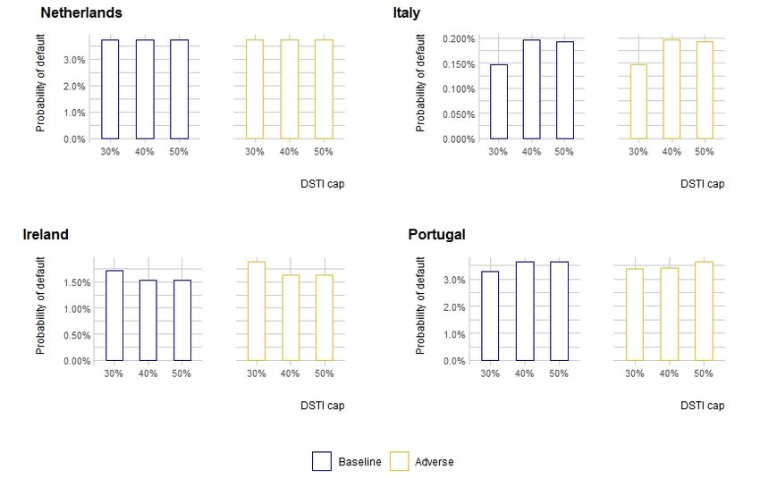
borrower-based MP measures and the adverse scenario with these measures in place. The
cost is computed in a similar fashion, as the difference in income (wealth) inequality between
the baseline scenarios with and without these MP measures in place. The only difference to
the benefits calculation is that the macroeconomic response is computed conditional on a loan
demand shock at MP measures introduction.

Results show that the imposition of the DSTI and LTV limits results in an increase in the
Gini coefficient of wealth ranging from 0.14 percentage points in Italy to 0.58 percentage points
in the Netherlands. In the baseline scenario with LTV and DSTI limits in place, two channels
affect household wealth. First, the wealth of all households is affected by the impulse response of
house, stock and bond prices to the loan demand shock implied by the borrower-based measures.
Second, the counterfactual value of wealth of excluded households decreases by the current house
value and increases by the initial mortgage amount. The change in wealth inequality is primarily
driven by the change in wealth of excluded households after imposition of borrower-based limits.
This welfare cost is expected given that (i) housing is the main source of wealth for households
in the low percentiles of the wealth distribution and (ii) borrower-based limits are more binding
for the latter households.

Somehow surprisingly, wealth inequality in the adverse scenario with borrower-based measures
in place is higher than in the adverse scenario without these limits. While low-wealth households
excluded from the mortgage market were shielded from a negative wealth shock following the
fall in house prices in the adverse scenario, the decrease in wealth resulting from barriers to
house ownership is larger. We derive the unconditional net benefit as the difference between the
expected value of the Gini coefficient with and without borrower-based measures, taking into
account the change in the crisis probability across policy scenarios. The unconditional benefit
of borrower-based measures in terms of wealth inequality ranges from -0.14 percentage points
in Italy to -0.58 percentage points in the Netherlands.

Turning to income inequality, a negligible decrease in the Gini coefficient of income is observed
after the imposition of LTV and DSTI limits, amounting to less than 0.04 percentage points in
the baseline scenario. The small impact on income inequality is due to the fact that two opposing
effects affect disposable income following the implementation of borrower-based limits. First,
borrower-based limits have a contractionary impact at introduction, resulting in an increase
in unemployment. Second, the debt burden decreases and therefore the disposable income of
excluded households increases. These two effects cancel each other out, resulting in a muted
impact on income inequality in the baseline scenario. In the adverse scenario income inequality
remains broadly unchanged. The main reason for this result is the negligible change in the
unemployment impulse response in the adverse scenario compared to the counterfactual with
borrower-based measures in place. The unconditional benefit of borrower-based measures in
terms of income inequality is less than 0.04 percentage points of the Gini coefficient of income.

ECB Working Paper Series No 2567 / June 2021                                                     4
These results suggest that the welfare costs of macroprudential regulation in terms of wealth
inequality are contained, while the benefits in terms of income inequality are negligible.

The remaining part of the paper is organised as follows: section 2 discusses how existing literature
informs our analysis, section 3 and 4 present the data and the methodology respectively, section
5 discusses the results and section 6 concludes.

2    Related Literature

The effect of macroprudential policy on inequality must be assessed considering the relation be-
tween financial crisis and inequality. If inequality makes a financial crisis more likely to happen,
then the welfare implications of central bank policies having distributional effects deserve more
attention, as they may increase the crisis probability. If on the other hand a financial crisis
results in a rise in inequality, then macroprudential measures may dampen the contractionary
effect of the crisis and mitigate the potential rise in inequality.

Based on existing evidence, it remains unclear whether inequality per se can be considered the
cause of the crisis or rather its consequence. Results from studies analyzing the direct impact of
inequality on the crisis probability find that a rise in income and wealth inequality is a predictor
of financial crisis (Kirschenmann et al. (2016), Perugini et al. (2016), Bellettini et al. (2019),
Paul (2020), Hauner (2020)). Since excessive credit growth has been identified as a robust
predictor of financial crisis (Schularick and Taylor (2012); Mian et al. (2017); Di Maggio and
Kermani (2017)), some authors have argued that inequality can lead to a financial crisis by
fuelling excessive credit growth. Empirical and theoretical evidence generally confirms that the
link between income inequality and debt accumulation is positive (Krueger and Perri (2006);
Iacoviello, M. (2008); Kumhof et al. (2015)). In contrast, Bordo and Meissner (2012) find that,
while credit booms heighten the probability of a banking crisis, income inequality does not
predict credit booms.

Similarly, the sign of the impact of a financial crisis on inequality is ambiguous. Some crisis lead
to a persistent increase in inequality (e.g. Asian financial crisis 1998, the post hyperinflation
period in CIS countries in 1990s), while other crisis have the opposite effect. The recent global
crisis for instance mitigated years of growing inequality in Brazil, since wealthy individuals were
more affected by the depreciation of stock exchanges and financial assets (Paiella and Salleo
(2019)). Analyzing a panel of OECD countries, Gokmen and Morin (2019) find that inequality
does not increase in the aftermath of the financial crisis. In advanced economies inequality tends
to decrease after stock market crashes, as wealthy people have higher investments in the stock
market. On average, inequality slightly decreases in the first year after the crisis and increases
in the years after (Čihák and Sahay (2020)).

Macroprudential policy can break the vicious link between inequality, indebtedness and financial

ECB Working Paper Series No 2567 / June 2021                                                      5
crisis. Several studies document the effectiveness of borrower-based macroprudential measures
in curbing credit growth (Bekkum et al. (2019); Ayyagari et al. (2017); Epure et al. (2018)). In
one study focusing on the UK mortgage market, the introduction of LTI limits leads to a lower
share of high LTI loans, in particular to low-income borrowers, and lowers house price growth
in the regions most affected by these measures. These regions experienced lower house price
corrections after the Brexit referendum and less mortgages defaults (Peydro et al. (2020)).

The literature on the distributional effects of central bank policies focused mostly on monetary
policy. For instance, nonstandard monetary policy seems to have a negligible effect on wealth
and income inequality (Lenza and Slacalek (2018)), while contractionary monetary policy shocks
have been found to increase income inequality Coibion et al. (2017)). Similarly, the cross-country
analysis in Furceri et al. (2018) shows that positive monetary policy shocks increase inequality,
in particular in countries with a high share of labor income and lower redistribution.

The distributional impact of macroprudential measures has received less attention. Some studies
pointed to the potential negative welfare effects of these policies in terms of wealth and income
inequality (Frost and Stralen (2018); Carpantier et al. (2016)). The reasoning is that borrower-
based measures such as loan-to-value (LTV) and debt-service-to-income (DSTI) limits may have
direct redistributive effects by excluding low income households from the mortgage market.
Frost and Stralen (2018) find that countries that use LTV and DSTI limits display higher (gross)
income inequality compared to countries that do not use these measures. In the same paper,
reserve requirements are associated with a lower income share for the bottom income deciles.
A negative association was observed between inequality on the one hand and the leverage ratio
and limits on foreign currency lending on the other hand. As pointed by the authors, causality
cannot be inferred from these results since country specific factors may determine the choice of
a specific macroprudential measure. A related study by Carpantier et al. (2016) calibrates a
theoretical model on household level data to explore the determinants of wealth inequality in
the presence of LTV limits. The study finds that LTV limits have a positive effect on wealth
inequality, while the bequest motive has a negative impact.

In this study, we use a counterfactual simulation to estimate the causal effect of the introduction
of borrower based macroprudential measures on wealth and income inequality under a baseline
and adverse macroeconomic scenario. We reasoned that, while borrower-based measures may
increase wealth inequality at introduction, they may act as a buffer during a financial crisis,
mitigating the resulting increase in inequality.

3    Data

The 2014 wave of the euro area Household Finance and Consumption Survey (HFCS) was used.
Table 6 shows the HFCS variables used in the simulations. We focus on four countries: Ireland,

ECB Working Paper Series No 2567 / June 2021                                                     6
Italy, Netherlands and Portugal. This heterogeneous group includes countries that recently
experienced a real estate crisis (Ireland), a sovereign debt crisis (Portugal, Ireland, Italy) as well
as well as a country with a high level of household indebtedness relative to GDP and no recent
history of a housing crisis (the Netherlands).3

Table 5 in the Appendix shows the summary statistics of wealth and income obtained from
the household data in the 4 countries of interest. The number of reporting households ranges
from 1,280 in the Netherlands to 8,037 in Italy. The median yearly gross income is significantly
higher in Ireland and the Netherlands compared to Italy and Portugal, at e41,472 and e49,095
versus e25,696 and e18,415 respectively. The ranking is similar in terms of total assets, with a
median values ranging from e161,986 in Portugal to e268,682 in the Netherlands. Median stock
holdings are the highest in Italy at e10,000, followed by median holdings of e3,000, e4,000 and
e8,000 in Portugal, Ireland and the Netherlands respectively.

The differences in household indebtedness are significant. The lowest level of outstanding mort-
gages is reported in Portugal, with a median outstanding mortgage of e90,450 representing
around 500% of yearly household income. In Ireland, Italy and the Netherlands median out-
standing mortgage amounts are e175,000, e100,000, and e151,000 respectively, representing
between 3 and 4 times the yearly household income. The median debt-service-to-income ratio
(DSTI) follows a similar pattern, ranging between 12% in Italy and 17% in Portugal.

Table 7 shows the summary statistics of selected variables by income percentile. As expected,
the value of the household residence is directly proportional to the household income. With the
exception of the Netherlands, the outstanding mortgage follows the same ranking. The LTV and
the DSTI decrease smoothly with the increase in income for all countries. The only exception is
the LTV for Italy which peaks for households in the 90th percentile of the income distribution.

Considering a typical LTV limit of 80% and a DSTI limit of 30%, table 7 suggests that the LTV
limit is by far the most binding constraint for all income percentiles, whereas the DSTI limit
is only binding for the 25th and to some extent for the 50th income percentile. Table 7 shows
how income and wealth inequality are linked. Low income households are also the ones with the
highest levels of indebtedness relative to their income and the assets they own. Therefore these
borrowers are the first to be affected by the imposition of borrower based measures, further
increasing the concentration of wealth among high-income borrowers.

Table 8 shows the distribution of the employment status by countries. For Ireland, Italy and the
Netherlands, the absolute difference between the unemployment rate derived from the HFCS
data and the aggregate unemployment rate measured in these countries on December 31, 2014
is between 2 and 3 percentage points (13.33%, 10.71%, 4.24% compared to aggregate rates of
10.91%, 12.72% and 7.15% for Ireland, Italy and the Netherlands respectively). In the case of
  3
   Netherlands has the highest level of household-debt-to GDP in the euro area, with values of 110%, 114% and
101% of GDP in the fourth quarter of 2006, 2016 and 2019 respectively.

ECB Working Paper Series No 2567 / June 2021                                                               7
Portugal, the HFCS unemployment figure of 13.21% comes the closest to the aggregate figure
13.54%.

Quarterly macroeconomic time series for real GDP, inflation, short-term interest rates, long-term
nominal yields (LTN), unemployment, loan volumes, loan interest rates, house prices, wages and
stock prices for the period ranging from September 1997 to December 2018 were obtained from
the ECB Statistical Data Warehouse. Bank level losses in the adverse scenario in the EBA 2018
Stress test were obtained from ECB internal models applied to stress test data submitted by
banks.

4    Empirical Approach

The empirical approach combines the method used by Gross and Poblacion (2017) and Lenza
and Slacalek (2018) for matching macro data with the HFCS data, as well as Budnik et al. (2014)
for the incorporation of the feedback loop between banks and the macroeconomy following the
adverse macroeconomic scenario. The approach includes several modules (see figure 1 below).

Each scenario starts with a loan demand or loan supply shock. In the baseline scenario, we
follow the approach of Gross and Poblacion (2017) and assume that the introduction of the
borrower-based measures is equivalent to a loan demand shock. The loan demand shock is
identified by constraining loan volume to fall together with lending rates in the first quarter of
the loan volume shock.

Similar to Budnik et al. (2014), we assume that the adverse macroeconomic scenario is followed
by a credit supply shock. Several studies document the importance of credit supply shocks
in the aftermath of the Great Financial Crisis, reflecting the emerging consensus according to
which banks are an independent source of shocks rather than just passive players transmitting
macroeconomic shocks (Nikolay et al. (2012), Fadejeva et al. (2017), Bijsterbosch and Falagia-
rda (2015)). These studies find that credit supply shocks have been an important driver of
business cycle fluctuations in the euro area, with a negative contribution in the aftermath of
the financial crisis. The transmission of the credit supply shock to the real economy is also
illustrated in studies based on micro-data such as Chodorow-Reich (2014) and Acharya et al.
(2018). Chodorow-Reich (2014) find that in the aftermath of Lehman bankruptcy, firms with
loans towards banks with a higher exposure to mortgage-backed securities reduced employment
by 4 to 5 percentage points more than banks with lower exposure to mortgage-backed securities.
Similarly, Acharya et al. (2018) find that firms with loans towards banks with higher sovereign
bond exposure during the sovereign debt crisis were less likely to obtain new loans, reducing their
investments and employment more than firms with creditors less exposed to sovereign bonds.

For identification, we impose the condition that a decrease in loan volumes is accompanied by
an increase in lending rates. To derive the size of the credit supply shock, we assume that

ECB Working Paper Series No 2567 / June 2021                                                     8
banks deleverage by the amount of loan losses incurred in the adverse scenario of the 2018
stress test. In the adverse scenario with borrower-based measures, the credit supply shock will
be correspondingly reduced: since borrower-based measures were introduced in the baseline
scenario, banks enter the crisis with lower credit risk parameters. The derivation of these new
credit risk parameters is described in the liquidity simulation module.

                                       Figure 1. Empirical approach

                         Adverse scenario                     Baseline scenario
                                       LTV/DSTI limit

                       yes                     no                        yes

               (Rescaled) loan        Loan supply              Loan demand
                supply shock             shock                    shock

                                     Unemployment                                     New wealth
                                  & asset price response                              distribution

                                 Unemployment simulation                           Liquidity simulation

                                 New income distribution                             Lower PD/LGD

In a next step, the response of house prices, stock and bond prices to the demand or supply
shock in each scenario are matched to the household level wealth data from the household survey
to obtain the new wealth distribution. Thereafter the unemployment response to the demand
and supply shocks in each scenario is used as input in the employment simulation. The latter
simulation is calibrated to the household level employment and demographic data to obtain a
new distribution of employment status. The employment status determines the household level
income, allowing the derivation of a new income distribution in each scenario.

4.1    Credit demand and supply shocks

We estimate a Bayesian Vector Autoregression (BVAR) to derive structural credit demand
(supply) shocks:
                                                        n
                                                        X
                                        Yi,t = ci +           Ai · Yi,t−j + εi,i                          (4.1)
                                                        j=1

ECB Working Paper Series No 2567 / June 2021                                                                 9
Where Yi,t is a vector of 10 macroeconomic variables including real GDP, inflation, short-term
interest rates, long-term nominal yields (LTN), unemployment, loan volumes, loan interest rates,
house prices, wages and stock prices and p is the number of lag variables. A Minnesota prior is
assumed for the residual covariance matrix. Under the Minnesota prior (Litterman, R. (1980),
Litterman, R. (1986)), it is assumed that residuals follow a multivariate normal distribution
with mean 0 and known variance-covariance matrix, while the endogenous variables present a
unit root in their own lags. Sign restrictions are imposed to identify supply and demand shocks
borrowing from the identification scheme in Hristov et al. (2011) (see table 9 in the Appendix).
We use the BEAR toolbox developed by Dieppe et al. (2016) for estimation.
The loan demand (supply) shocks correspond to the 3 different policy scenarios as shown in
table 1 below. The imposition of LTV and DSTI limits is assumed to be equivalent to a credit
demand shock equal to the loan volume excluded after the imposition of the limits. We focus
on mortgages from the HFCS data set issued in 2006, just before the financial crisis. In turn,
the credit supply shock in the adverse scenario is derived from the bank level losses reported in
the 2018 stress test adverse scenario aggregated at country level. It is assumed that following
the adverse scenario, banks reduce lending by an amount equal to the incurred losses. The
scaled supply shock in the adverse scenario with borrower-based measures is obtained by scaling
the losses reported by banks in the adverse scenario with the relative change in credit risk
parameters induced by LTV and DTSI limits imposition (default probability, PD and loss-given
default, LGD) as described in the liquidity simulation module.
Table 1: Overview of scenarios
Macro scenario Policy scenario Type of shock
Baseline LTV/DSTI = No -
Baseline LTV/DSTI = Yes Loan demand
Adverse LTV/DSTI = No Loan supply
Adverse LTV/DSTI = Yes Loan supply
The response of unemployment and wages to the scenario conditional demand (supply) shocks
is used as input in the unemployment simulation to derive a new income distribution. The
response of house prices, stock and bond prices is used as input for the derivation of a new
wealth distribution in each scenario. The initial income and wealth distribution is obtained
from the HFCS data.
4.2 Employment simulation
In this module, the response of macroeconomic variables to the scenario specific demand and
supply shock is mapped to the employment distribution of households in the HFCS dataset.
ECB Working Paper Series No 2567 / June 2021 10The probability of being employed is a latent unobservable variable (yi∗ ), which is assumed to
be a function of workers demographics:
yi∗ = Xi β + εi (4.2)
Where εi follows a logistic distribution and vector X includes demographic variables for each
individual i such as gender, age, education, marital status, a dummy variable taking the value
1 if the host country is the country of birth and 0 otherwise, as well as a constant term. The
sample for the regression in equation 4.2 only includes the active population, excluding students,
retirees and any other individuals who are unable to work.
Since employment status is observed, while individual employment probability is not, we assume:
1 (employed) if yi∗ ≥ 0
yi = (4.3)
0 (unemployed) if yi∗ ≤ 0
The regression 4.2 is estimated at country level using the Maximum Likelihood (ML) method.
The dependent variable is a binary vector that takes value 1 if the individual i is employed and 0
otherwise. The estimated parameters β̂ from equation 4.2 are plugged into the logistic function
to obtain individual employment probabilities p̂emp
i :
1
p̂emp
i = (4.4)
1 + e−Xi β̂
The probabilities p̂emp
i are used to simulate employment status by comparing them to random
draws from a uniform distribution in the [0, 1] interval. Following Gross and Poblacion
(2017) and Lenza and Slacalek (2018), an individual is employed if p̂emp
i > . An individual’s
employment status does not change in the baseline scenario. In all other scenarios, individuals
will either remain employed or transition into unemployment, depending on the outcome of the
simulation.
The intercept of the logistic regression is adjusted to match the aggregate unemployment rate
obtained from the BVAR under each policy scenario. Different from Gross and Poblacion (2017),
the intercept varies for low income versus high income individuals, such that the intercept for
the low income individuals represents 88% of aggregate unemployment. The differentiation
between low income and high income individuals is meant to account for the fact that low
income individuals experience higher unemployment than high income individuals, in particular
after a recession. The intercepts were calibrated based on data from the Dutch household survey
showing that low income individuals account for 88% of the increase in the unemployment in
ECB Working Paper Series No 2567 / June 2021 11the Netherlands in the 7 years after the 2009 recession.4 Low income is defined as income lower
than the bottom 25 percentile of the country’s income distribution.
4.3 Liquidity simulation
This module is used to derive the scaling factor for the credit supply shock in the adverse scenario
with borrower-based measures. The scaling factor is derived from the ratio between the average
credit losses with and without MP measures in the baseline scenario. Essentially, the scaling is
equivalent to a starting point adjustment in the adverse scenario with borrower-based measure
in place, since banks enter the adverse scenario with lower PD and LGD parameters. Lower
credit losses in the adverse scenario imply a lower need for deleveraging and therefore a lower
credit supply shock:
pdhh st
M P · lgdM P
cla,M P = clast · (4.5)
pdhh · lgdst
Where cla,M P represents credit losses in the adverse scenario with MP measures in place, cla
the credit losses reported by banks in the EBA 2018 stress test, pdhh is the household default
probability computed from the HFCS data conditional on MP measures, pdhh
M P is the household
default probability as implied by the HFCS data, lgdst the starting point LGD reported by
banks in the 2018 stress test and lgdst
M P the rescaled starting point LGD that reflects the lower
LTV resulting from the imposition of the borrower-based measures.
The default probability pdhh
s of household hh in scenario s is defined as the sum of households
that become illiquid in the simulation horizon (12 quarters) over the total number of households.
The household will become insolvent if its liquidity inflows are lower than its liquidity outflows.
Households’ liquidity is simulated under the baseline scenario with and without MP measures
in place.
The following 4 inputs are required for the liquidity simulation: (i) the employment simulation
results from section 4.2, aggregated at household level, (ii) an unemployment benefit vector for
the entire sample of active population and (iii) an employment income vector for the entire
sample of active population and (iv) the change in the value of liquid assets, where liquid assets
are defined as the sum of cash, bonds and stocks holdings.
Since default probabilities are estimated from the bank’s perspective, we do no allow for any
role of liquid assets to smooth consumption. Creditors will only have recourse to assets pledged
as collateral in case of borrower default. Given that the liquidation of collateral is a lengthy
and costly procedure, banks typically only consider income and not assets for the assessment of
borrower creditworthiness in a loan application.
4
The ratio has a value of 80% in 2009 and reaches 87% in 2015.
ECB Working Paper Series No 2567 / June 2021 12The unemployment benefit transfers and employment wages are obtained from the HFCS sur-
vey data. The salaries of individuals’ transitioning to unemployment under each scenario are
replaced with their estimated unemployment benefits. These benefits are assumed to be a
function of workers past employment salaries. Given that each country has their own national
unemployment scheme, the transfers are calculated replicating each country’s methodology.5
Missing employment income observations are imputed using predicted values from a regression
having the HFCS reported annual employment salary as a dependent variable and demographic
variables including gender, age, education, marital status and a dummy variable indicating
whether the host country is the country of birth as predictors.
Once all three inputs are defined, labor income is computed as follows:
incls,i = emps,i · incemp
i · (1 + γswage ) + (1 − emps,i ) · transfiunemp (4.6)
Where emps,i is the employment indicator for individual i in scenario s obtained in section
4.2 and takes the value 1 if the individual is employed and 0 otherwise, γswage is the scenario-
specific 12-quarter impulse response of wages and incemp
i and transfiunemp are the individual
employment salary and unemployment benefit, respectively, as described above.
Thereafter, results are aggregated at the household level by pooling together all the individuals
who belong to the same household. In addition to labor income, total household level income is
computed considering any other income sources households report in the HFCS Survey:
inctot l oth
s,hh = incs,hh + incs,hh (4.7)
Where incoth
s,hh represents any other sources of income (pension, real estate property income,
social transfers other than unemployment or regular private transfers).
The next step in the liquidity simulation, is to calculate the 12-quarter-change of the market
value of households’ stocks and bond holdings:
∆bhh,s = bhh · γsb and ∆shh,s = shh · γss (4.8)
Where bhh indicates bond holdings, γsb is the scenario-specific 12-quarter-impulse response on
bond yields, shh represents stock holdings, γss is the scenario-specific 12-quarter-impulse response
on stock prices.
5
An overview of OECD countries’ National Unemployment Schemes can be accessed under the following
link: http://www.oecd.org/social/benefits-and-wages.The transfers are computed following each country’s
methodology as they stand as of August 2020.
ECB Working Paper Series No 2567 / June 2021 13The household level liquidity status is computed as the difference between household’s total in-
come and total expenditures. Expenditures include debt repayments such as mortgage payments
for households with outstanding mortgages, house rental payments and expenses for consump-
tion of goods and services:
out rep
∆liqs,hh = inctot excl cons
s,hh + ∆bhh,s + ∆shh,s − (1 − Ihh,s ) · min(dhh , dhh ) − exphh (4.9)
Where Isexcl represents a binary vector taking the value 1 if the household had a mortgage
outstanding that did not satisfy the new LTV and DSTI limit under scenario s and 0 otherwise,
drep out cons
hh indicates the monthly debt payment, dhh indicates total outstanding debt and exphh
represents households’ monthly consumption on goods and services.6 All variables are adjusted
to monthly values.
If the liquidity of a household becomes negative as a result of the macro-financial conditions of
each scenario, the individual is unable to meet its outstanding debt payment obligations and is
therefore considered to be in default. The default probability P D is defined as the sum of the
number of defaulting households relative to the total number of households in the country Nc .7
hh 1 Nc
P Dc,s = Σ 1∆liqs,hhrelative change in the LGD is computed by adjusting the LTV reported by banks with the
relative change in the average country LTV obtained from the HFCS data after imposition of
the LTV limit.
All calculations are initially run using a grid for the LTV limit ranging from 50% to 90% and
a DSTI limit ranging from 30% to 50%. Given that final results do not change materially for
different DSTI values, cost benefit calculations are performed with a constant DSTI limit at
30% and a LTV limit at 80%.
Finally, the relative change in the product of the aggregate PD and LGD in the baseline scenario
with and without MP measures is used for the scaling of the credit supply shock in the adverse
scenario in equation 4.5.
4.4 Net benefit of borrower-based measures
In the last step, the wealth and income distributions derived in each scenario are used to compute
income and wealth inequality. Inequality is assessed using the Gini coefficient. Alternative
measures of inequality, such as the ratio between the 75th and the 25th percentile of the income
and wealth distribution are used. The results remain qualitatively unchanged.
The benefit of borrower based measures in terms of wealth inequality is computed as the dif-
ference between the Gini coefficient in the adverse scenario without and with borrower-based
measures in place:
bw,M P = giniw w,M P
a − ginia (4.13)
Similarly, the cost of borrower based measures is computed as the difference between the Gini
coefficient in the baseline with and without borrower-based measures in place:
cw,M P = giniw w
w,M P − ginib (4.14)
Where giniw,M
a
P
and giniw
a refer to the wealth-based Gini coefficients with and without borrower-
based measures in place in the adverse scenario respectively, while giniw,M
b
P
and giniw
b refer to
the wealth-based Gini coefficients with and without borrower-based measures in place in the
baseline scenario. The calculations are performed analogous for the costs and benefits with
respect to income inequality.
The calculations above estimate the benefit conditional on a crisis. The unconditional benefit is
computed as the difference between the expected values of the Gini coefficient with and without
borrower-based measures, taking into account the change in the crisis probability across policy
scenarios:
ECB Working Paper Series No 2567 / June 2021 15b̂w,M P = (p · giniw w − pM P · giniw w
a + (1 − p·) ginib ) a,M P + (1 − pM P ) · ginib,M P (4.15)
Where pM P and p refer to the crisis probability with and without borrower-based measures
in place respectively. The first bracket shows the expected Gini coefficient of wealth without
borrower-based measures in place. The second bracket shows the expected Gini coefficient of
wealth with borrower-based measures in place.
Similarly, the unconditional benefit in terms of income inequality is computed as:
b̂i,M P = p · giniia + (1 − p·) giniib − pM P · giniia,M P + (1 − pM P ) · giniib,M P
(4.16)
The crisis probability is computed as the fitted value from the model by Schularick and Taylor
(2012). The crisis probability in their model is a function of the log changes in the credit-to-
GDP ratio. The model is estimated for 14 advanced economies over the period 1870–2008. Since
credit growth and the crisis probability are negatively correlated, the loan demand shock after
imposition of LTV and DSTI measures in the baseline scenario will lead to a reduction in the
crisis probability, changing the expected gini coefficient.8
5 Results and Discussion
5.1 Credit demand and supply shocks
Figures 9 and 10 in the Appendix report the cumulative impulse responses conditional on a one
standard deviation loan demand and supply shock respectively.
The impulse responses in each scenario are scaled with the scenario specific change in loan
volume, expressed in loan growth standard deviations. In the case of the loan demand shock, an
LTV limit of 80% in combination with a DSTI limit of 30% implies a decrease in loan volume of
7.6% for Ireland, 5.36% for Italy, 4.46% for Portugal and 5.05% for the Netherlands.9 Expressed
in standard deviations of loan growth, the latter change in loan volume corresponds to 1.7
standard deviations in Ireland, 2.5 in Italy, 4.9 in Portugal and 2.3 in the Netherlands.
In turn, the magnitude of the loan supply shock is given by the amount of credit losses incurred
by banks in the adverse scenario in the 2018 stress test. These credit losses are equivalent to a
8
To estimate fitted values of the crisis probability, we used specification number (9) in table 4 as it performed
better than the specifications using credit growth as predictors.
9
The change in loan volume implied by the combination of the 80% LTV and 30% DSTI limit is only applied
to the share of loans represented by mortgages. The mortgage share ranges from 0.55 in Portugal to 0.65 in the
Netherlands.
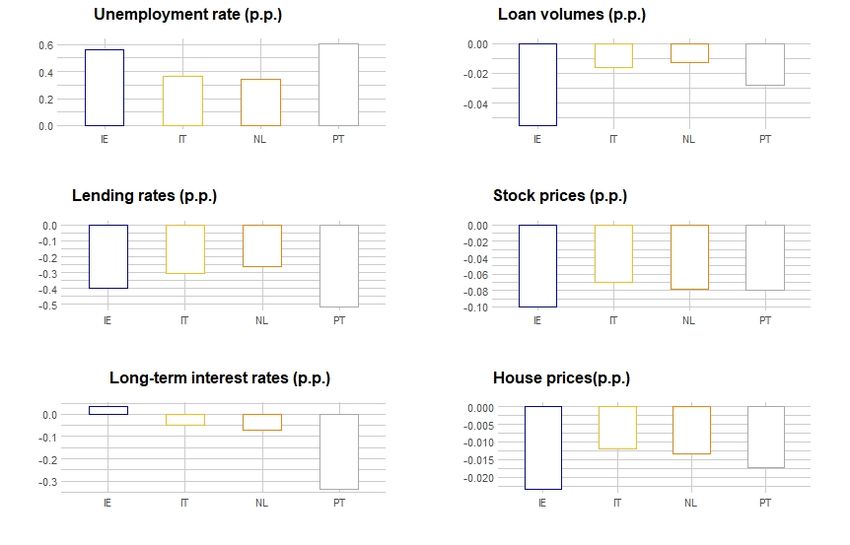
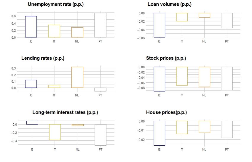
ECB Working Paper Series No 2567 / June 2021 16Figure 2. Impulse Responses. Unemployment rate Note: The chart shows the scaled impulse responses of unemployment for the different scenarios. The impulse response calculation from the BVAR is described in section 4.1. decrease in loan volume, ranging from 0.85% in the Netherlands to 2.34% in Italy. Expressed in standard deviations, the decrease in loan volume ranges from 0.4 standard deviation in the Netherlands to 1.5 in Portugal. In the adverse scenario with borrower-based measures in place, mortgage credit losses are scaled down with a factor computed as in equation 4.5, reflecting the lower credit risk parameters implied by the borrower-based measures. The scaling factor ranges from 0.5 in Italy to 0.9 in Ireland and is applied to the share of mortgage losses out of total credit losses in the adverse scenario.The share ranges from 0.1 in Italy to 0.3 in Ireland. Figures 2, 3, 4 in this section and figure 11 in the Appendix report the scaled impulse responses by scenario for each of the main 4 variables of interest: unemployment, house prices, stock prices and long-term nominal yields. After imposition of borrower-based measures in the baseline scenario, the unemployment response ranges from 0.8 percentage points in the Netherlands to 1 percentage point in Ireland. In contrast, the unemployment response after the adverse scenario loan supply shock is considerably lower, ranging between 0.1 percentage points in the Netherlands to 0.4 in Portugal and Italy. The material difference between the unemployment response in the two scenarios above is the significantly higher contraction in credit in the baseline scenario with borrower-based measures in place compared to the adverse scenario. The largest gap can be observed in Ireland, with a ECB Working Paper Series No 2567 / June 2021 17
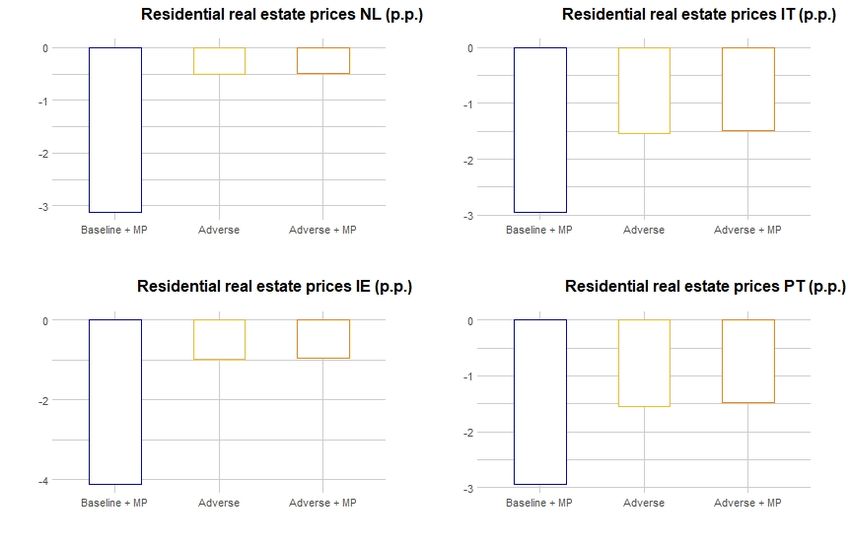
Figure 3. Impulse Responses. Residential real estate prices

Note: The chart shows the scaled impulse responses of house prices rates for the different scenarios. The impulse
response calculation from the BVAR is described in section 4.1.

7% loan contraction in the baseline with macroprudential measures versus 1.6% in the adverse
scenario. The supply shock driven contraction of credit in the adverse scenario is comparable
with the estimates by Nikolay et al. (2012), yet significantly lower than estimates of Bijsterbosch
and Falagiarda (2015) during the crisis period. Due to the low weight of the mortgage credit
losses in combination with the moderate response of risk parameters,10 the unemployment re-
sponse for the adverse scenarios with and without borrower-based measures in place is almost
identical. The unemployment response across scenarios is the main driver for the changes in
income inequality reported in section 5.4.

The same pattern discussed for the unemployment response can be observed for the house prices.
The impulse response of house prices to a one standard deviation loan demand shock ranges from
-2.3 percentage points in Ireland to -1.1 percentage points in Italy (figure 9 in the Appendix).
After imposition of borrower-based limits in the baseline scenario, the house price correction
ranges from -2.9 percentage points in Portugal to -4.1 percentage points in Ireland (figure 3).
Following the credit supply shock in the adverse scenario, the drop in house price is significantly
lower, with values between -0.5 percentage points in the Netherlands to -1.5 percentage points
  10
     See figures 7 in the next section and figure 12 in the Appendix for a comparison of the change in risk parameters
after introduction of the LTV and DSTI limits across countries.

ECB Working Paper Series No 2567 / June 2021                                                                       18
in Portugal (3). As expected, the figures for the adverse scenario with borrower-based measures
in place are almost identical to the adverse scenario estimates.
Figure 4. Impulse Responses. Stock prices
Note: The chart shows the scaled impulse responses of unemployment for the different scenarios. The impulse
response calculation from the BVAR is described in section 4.1.
The stock price decrease following the MP limits implied loan demand shock amounts to around
-18 percentage points in Ireland and the Netherlands and around -17 percentage points in Italy
and Portugal. In the adverse scenario, the house price drop is less severe, at around -3 percentage
points in Ireland and the Netherlands and -7 percentage points in Italy and Portugal. Last, the
response of the long term nominal (LTN) rates to the MP limits implied loan demand shock
amounts to -0.1 percentage points. The loan supply shock in the adverse scenario results in
a LTN drop 0.4 of percentage points in Italy and Portugal and an increase of 0.03 percentage
points in Ireland. The response in the adverse scenario with MP limits is almost identical.
The rescaled impulse responses are added to the level of the macroeconomic variable specified
by the EBA scenario. The resulting set of macroeconomic variables account for the feedback
between the banking sector and the macro economy following the adverse scenario. The unem-
ployment response is a key input for the employment and the liquidity simulation, ultimately
determining the income distribution in each scenario. The asset price changes are used as input
to determine the new wealth distribution in each scenario.
ECB Working Paper Series No 2567 / June 2021 195.2 Employment simulation
The results of the logistic regression from equation 4.2 are reported in table 2.
Table 2: Employment probability
Variable IE IT NL PT
Intercept 0.37*** -1.39*** 2.92*** -0.02
(0.08) (0.14) (0.53) (0.14)
Age - 0.05*** -0.02* 0.01***
(0.00) (0.01) (0.00)
Male -0.10 0.08 -0.23 0.10
(0.06) (0.06) (0.24) (0.06)
Marital status 0.99* 0.74* 0.65 0.75*
(0.06) (0.07) (0.25) (0.06)
Education 1.21* 0.78* 0.18 1.11*
(0.07) (0.09) (0.24) (0.08)
Country birth 0.31* 0.00* 0.28 0.14*
(0.08) (0.09) (0.3) (0.09)
Note: This table reports the results of the logistic regression having the employment status as a dependent vari-
able and age, education, gender as covariates. Country birth is a dummy variable indicating taking the value 1 if
the host country is the country of birth and 0 otherwise.
Married and individual with a high level of education are more likely to be employed. Similarly,
being born in the host country increases the probability of being employed. The coefficients
of these variables are positive and weakly significant in all countries except the Netherlands.
Men are more likely to be employed in Italy and Portugal and more likely to be unemployed in
Ireland and the Netherlands, but the effect is not statistically significant. Finally, older people
are more likely to be employed in Italy and Portugal, while in the Netherlands the opposite is
the case. No data on age was available for Irish respondents.
The results of the unemployment simulation are shown in figure 5, separately for low income
and high income individuals. The scenarios with borrower-based measures assume an LTV
limit of 80% and a DSTI limit of 30%. Results remain qualitatively unchanged for different
combinations of the LTV/DSTI limits. In the case of low income individuals, the imposition of
borrower based measures in the baseline scenario leads to an increase in unemployment ranging
between 0.3 percentage points in Ireland to 0.6 percentage points in Portugal. In the adverse
scenario with LTV/DSTI limits in place, the decrease in unemployment compared to the adverse
scenario without DSTI/LTV limits ranges between 0.02 in Ireland and 0.2 percentage points in
Portugal (lower panel). For high income individuals, the impact is negligible, the increase in
the baseline ranges between 0.03 in Italy and 0.08 percentage points in Portugal, while in the
adverse scenario the impact is close to 0 in 3 out of 4 countries (upper panel).
ECB Working Paper Series No 2567 / June 2021 20Figure 5. Impact of DSTI/LTV limits on unemployment
Note: The upper panel shows the results of the unemployment simulation for high income individuals across
policy scenarios. The lower panel shows the results of the unemployment simulation for low income individuals.
Low income individuals are those with an income lower than the 25t h percentile of the country distribution. The
scenario with borrower-based measures in place (’MP’) assumes an LTV limit of 80% and a DSTI limit of 30%.
5.3 Liquidity simulation
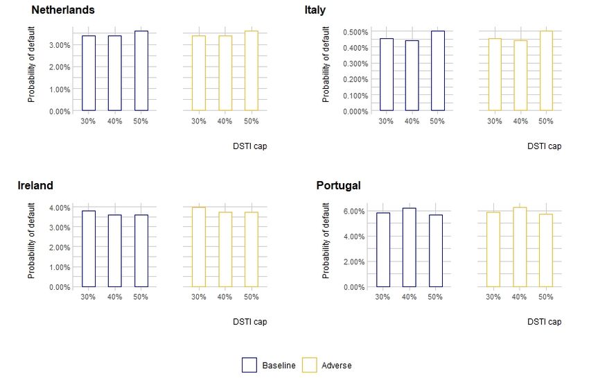
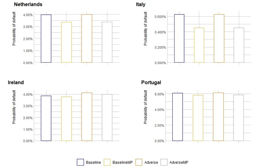
Figure 6 shows the default probability (PD) with and without borrower-based measures assuming
a DSTI limit of 30% and an LTV limit of 80% in the adverse and baseline scenario.11 Figure 12
in the Appendix shows the PD for different DSTI limits.
The impact of macroprudential measures on the default probability is ambiguous. Since a lower
debt burden eases household budget constraints, exclusion from the mortgage market is expected
to decrease the default probability. On the other hand, since the loan demand shock implied
by the LTV/DSTI measures has a small contractionary effect, as shown by the increase in
unemployment in figure 10, default probability may increase after the introduction of borrower-
based measures. The counter-intuitive decrease in the PD as the DSTI limit is relaxed in the
case of Ireland illustrates this trade-off (see figure 12).
11
The low PD in Italy is driven by the relative high weight of bond holdings relative to other countries and the
high long term nominal yield of Italy in the baseline scenario, with a value of 4.2 p.p. versus 1.1, 1.7 and 3 p.p.
in the Netherlands, Ireland and Portugal respectively. The high weight of bond holdings combined with a high
sovereign bond yield for Italy results in a PD of 0.26% in the baseline scenario compared to 1.78% for Ireland and
3.78% for Portugal.
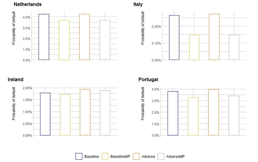
ECB Working Paper Series No 2567 / June 2021 21Figure 6. Impact of macroprudential policy regimes on PDs Note: The chart shows the PD before and after the imposition of a DSTI limit of 30% and LTV limit of 80% under both macroeconomic scenarios. The PD is obtained from the liquidity simulation in section 4.3. The PD and LGD estimates above are used to derive a scaling factor for the credit supply shock in the adverse scenario with borrower-based measures in place. The scaling factor was determined as the product of the ratios of PD and LGD with and without borrower-based measures in place assuming an LTV limit of 80% and a DTSI limit of 30%. The factor has a value of 0.5 for Italy, around 0.85 for Ireland and Portugal and 0.9 for the Netherlands. Figure 7 shows the ratio between the LGD with and without borrower-based measures in place for an DSTI limit of 30% and an LTV limit ranging between 50% and 90%. Note that only mortgages issued in 2006 were considered, which considerably reduces the scope of eligible mortgages for this analysis. As expected, both the PD and the LGD decrease after the LTV/DSTI limits are imposed. The LGD increases monotonously as the LTV limit is relaxed, while the PD increases in the DSTI limit (see figures 7 and 12). These results are consistent with the findings from Gross and Poblacion (2017) indicating that the DSTI limits have a stronger negative impact on the PD while the LTV limit leads to a higher reduction in the LGD. ECB Working Paper Series No 2567 / June 2021 22
Figure 7. Impact of LTV limits on LGDs

Note: The chart shows the ratio between the LGD after the imposition of the DSTI and LTV limit using as
input (i) the starting point LGDs reported by banks in the 2018 stress test and (ii) the relative decrease in the
average country LTV after imposition of the LTV limits as implied by the HFCS data.

                                       Figure 8. Crisis probability

Note: The figure shows the crisis probability conditional on the introduction on the borrower-based measures.
The crisis probability is computed as indicated in section 4.4. using the model by Schularick and Taylor (2012).
A DSTI limit of 30% was assumed.

ECB Working Paper Series No 2567 / June 2021                                                                   23
Turning to the crisis probability conditional on the introduction of borrower-based measures, chart 8 shows that the crisis probability experiences a significant drop across the values of the LTV limits considered. The baseline crisis probability ranges from 1.01% in the Netherlands to 2.24% in Ireland. After the imposition of the DSTI/LTV limits, the absolute drop in the crisis probability ranges from 0.26 percentage points in the Netherlands to 0.9 percentage points in Ireland. These probabilities will be used in the next section for the cost-benefit calculations. 5.4 Costs and benefits of borrower-based measures Turning to the main question of this study, this section analyzes the distributional consequences of the imposition of DSTI and LTV limits under different macroeconomic scenarios. The results presented in this section refer to a cap of 80% and a DSTI limit of 30% for mortgages issued in 2006. Tables 11 in the Appendix shows the wealth distribution and the relative change in wealth after LTV and DSTI limits imposition in the baseline scenario. With the exception of Italy, exclusion from the mortgage market has a lower relative impact on high-wealth households (75th and 90th percentile) compared to low-wealth households (25th and 50th percentile). In Italy, households in the 90th percentile see their wealth decrease by 2.5%, compared to only 1.1% for households in the 25th percentile of the wealth distribution. For all countries except Portugal, the wealth impact peaks for households in the 50th percentile, with a decrease in wealth ranging from -2.8% in Italy to -6.9% in the Netherlands. In Portugal, the largest wealth impact of the imposition of borrower-based measures is for households in the 25th percentile, with a decrease in wealth of -12.4%. Two channels affect household wealth in the baseline scenario with LTV and DSTI limits. First, the wealth of all households is affected by the impulse response of house, stock and bond prices to the loan demand shock implied by the borrower-based measures. Second, the wealth of excluded households decreases by the current house value and increases by the initial mortgage amount. The change in wealth inequality is primarily driven by the change in wealth of excluded households after imposition of borrower-based limits. This is because housing represents a larger share of wealth for households in the lower compared to households in the upper percentiles of the wealth distribution. The former households are also more likely to be affected by the imposition of borrower-based limits (table 7 in the Appendix). Table 3 reports the Gini coefficient of wealth across the four combinations of macroeconomic and policy scenarios. In the baseline scenario, the imposition of the DSTI and LTV limits results in an increase in the Gini coefficient ranging from 0.14 percentage points in Italy to 0.58 percentage points in the Netherlands. This difference is carried over in the adverse scenario, with wealth inequality with borrower-based measures in place between 0.03 and 0.43 percentage points higher than in the counterfactual adverse scenario without these measures. ECB Working Paper Series No 2567 / June 2021 24
Wealth inequality in the adverse scenario with borrower-based measures in place is higher than
in the adverse scenario without these limits. Low-wealth households that were excluded from the
mortgage market in the counterfactual baseline scenario were shielded from a negative wealth
shock due to the drop in house prices in the adverse scenario. Nevertheless, the decrease in wealth
resulting from not owning a house in the first place is larger. The unconditional net benefit is
computed as the difference between the expected value of the Gini coefficient with and without
borrower-based measures, taking into account the change in the crisis probability across policy
scenarios, as in equation 4.15 (see column (7) in table 3). The unconditional benefit is negative
in all countries, ranging from -0.14 percentage points in Italy to -0.58 percentage points in the
Netherlands. After considering the decrease in the crisis probability following the imposition of
borrower-based measures, the positive impact on wealth inequality resulting from LTV and DTSI
limits imposition in the baseline scenario dominates the negative effect on inequality resulting
from lower house price shocks in the adverse scenario.

                            Table 3: Net wealth inequality across scenarios

                        (1)         (2)          (3)       (4)       (5)       (6)         (7)
          Scenario    Baseline    Baseline      Cost     Adverse   Adverse   Benefit   Net benefit
                      MP=no       MP=yes       (2)-(1)   MP=no     MP=yes    (4)-(5)   (uncond.)
          IE          67.14%      67.69%       0.54%     67.17%    67.41%    -0.24%     -0.54%
          IT          58.74%      58.88%       0.14%     58.80%    58.82%    -0.03%     -0.14%
          NL          56.54%      57.12%       0.58%     56.59%    57.02%    -0.43%     -0.58%
          PT          65.28%      65.68%       0.40%     65.47%    65.54%    -0.09%     -0.40%

Note: The table reports the Gini coefficient of net wealth across the 4 combinations of macroeconomic
and macroprudential policy scenarios. The unconditional benefit in the adverse scenario represents an
expected value and is computed as in equation 4.15.

Table 12 in the Appendix shows total income distribution and the relative change in income
after LTV and DSTI limits imposition in the baseline scenario. The magnitude of the income
decrease is significantly lower compared to the decrease in wealth. The reason for the muted
impact of the borrower-based measures on income is that two opposing effects are at play. The
decrease in debt burden of excluded households increases available income, while the increase
in unemployment resulting from the loan demand shock tends to decrease available income.
The two effects cancel each other out, resulting in a marginal change in income. For the most
affected income segment, the 50th percentile, the impact ranges between -0.33 percentage points
in Portugal to -0.53 percentage points in the Netherlands. The only exception is Ireland for
which the strongest impact is observed for households situated in the 75th and 90th percentile
of the income distribution.

Table 4 reports the Gini coefficient of income across the four combinations of macroeconomic
and policy scenarios. In the baseline scenario, a negligible decrease in the Gini coefficient is
observed after LTV and DSTI limits imposition, amounting to less than 0.04 percentage points.

ECB Working Paper Series No 2567 / June 2021                                                         25
You can also read