Ifo WORKING PAPERS Financial Bubbles in Interbank Lending - CESifo Group Munich
←
→
Page content transcription
If your browser does not render page correctly, please read the page content below
ifo                               260
                                 2018
WORKING                           April 2018

PAPERS
 Financial Bubbles in Interbank
 Lending
 Luisa Corrado, Tobias Schuler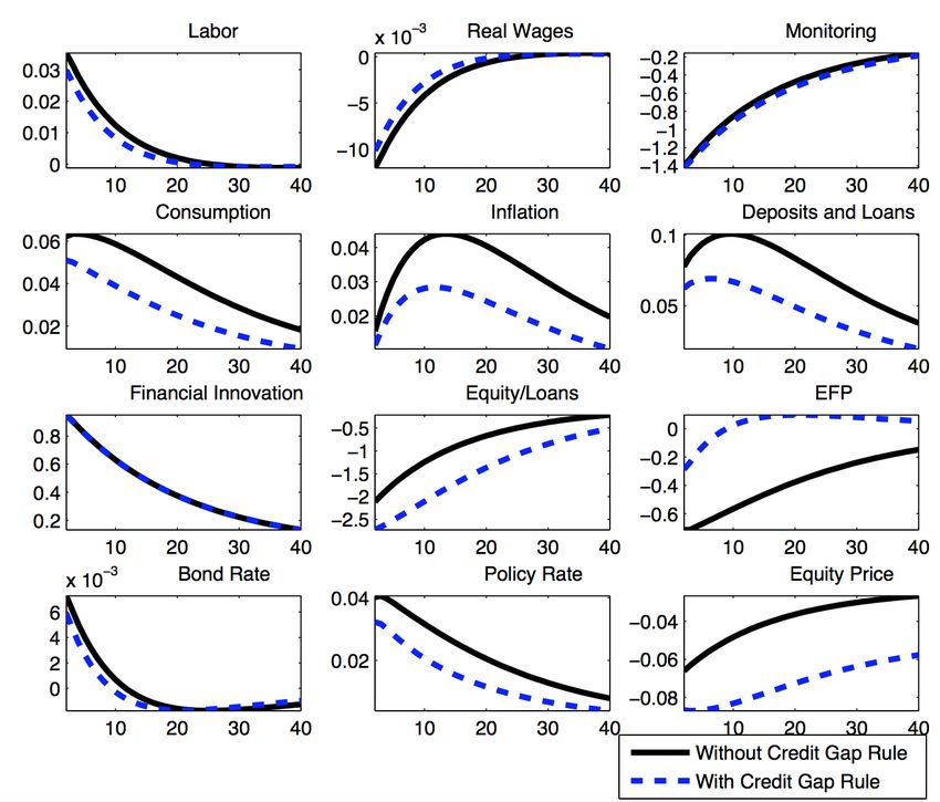
Impressum:

ifo Working Papers
Publisher and distributor: ifo Institute – Leibniz Institute for Economic Research at the
University of Munich
Poschingerstr. 5, 81679 Munich, Germany
Telephone +49(0)89 9224 0, Telefax +49(0)89 985369, email ifo@ifo.de
www.cesifo-group.de

An electronic version of the paper may be downloaded from the ifo website:
www.cesifo-group.de
ifo Working Paper No. 260 (Apr 9, 2018)

                       Financial Bubbles in Interbank Lendingi

                                                 Abstract

As a result of the global financial crisis countercyclical capital requirements have been
discussed to prevent financial bubbles generated in the banking sector and to mitigate
the adverse effects of financial repression after a bubble burst. This paper analyses the
effects of an endogenous capital requirement based on the credit-to-GDP gap along
with other policy instruments. We develop a macroeconomic framework which endo-
genizes market expectations on asset values and allows for interbank transactions. We
then show how a bubble in the banking sector relaxes financing constraints. In policy
experiments we find that an endogenous capital requirement can effectively reduce the
impact of a financial bubble. We show that central bank intervention (\leaning against
the wind") instead has only a minor effect.

JEL Code: E44, E52
Keywords: Financial bubbles, credit-to-GDP gap, endogenous capital requirement,
stabilization policies

                Luisa Corrado                                             Tobias Schulerii
    Department of Economics and Finance                         ifo Institute – Leibniz Institute for
       University of Rome Tor Vergata                                   Economic Research
                via Columbia 2                                      at the University of Munich
              00133 Rome, Italy                                           Poschingerstr. 5
             T +39 067259-5734,                                      81679 Munich, Germany
          luisa.corrado@uniroma2.it                                     T +49 89-9224-1239
                                                                           Schuler@ifo.de

i
   We would like to thank Jeffrey Campbell, Michael Kumhof, Stephen Millard, Tommaso Proietti and Radek Sauer
for helpful comments, as well as participants at the Monetary and Macroeconomics seminar at the Bank of Eng-
land, and during presentations at the University of Rome Tor Vergata, the EEA-ESEM annual congress 2017, the
EconPol Europe Founding Conference 2017, and ifo Macroeconomics Seminar 2018. We acknowledge research
assistance by Tim Stutzmann. The usual disclaimer applies.
ii
   Corresponding author.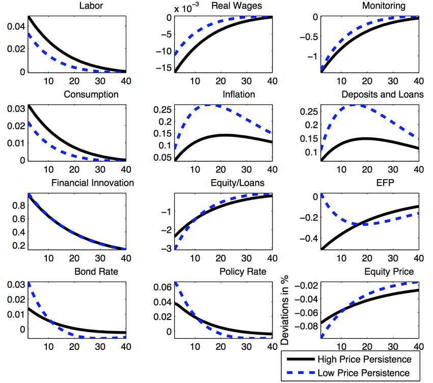
Financial Bubbles in Interbank Lending∗
                           Luisa Corrado†                Tobias Schuler‡

                                           April 9, 2018

                                               Abstract

          As a result of the global financial crisis countercyclical capital requirements
      have been discussed to prevent financial bubbles generated in the banking sector
      and to mitigate the adverse effects of financial repression after a bubble burst.
      This paper analyzes the effects of an endogenous capital requirement based on the
      credit-to-GDP gap along with other policy instruments. We develop a macroe-
      conomic framework which endogenizes market expectations on asset values and
      allows for interbank transactions. We then show how a bubble in the bank-
      ing sector relaxes financing constraints. In policy experiments we find that an
      endogenous capital requirement can effectively reduce the impact of a financial
      bubble. We show that central bank intervention (“leaning against the wind”)
      instead has only a minor effect.

      JEL: E44, E52
      Keywords: Financial bubbles, credit-to-GDP gap, endogenous capital require-
      ment, stabilization policies

  ∗
     We would like to thank Jeffrey Campbell, Michael Kumhof, Stephen Millard, Tommaso Proietti and
Radek Šauer for helpful comments, as well as participants at the Monetary and Macroeconomics seminar
at the Bank of England, and during presentations at the University of Rome Tor Vergata, the EEA-ESEM
annual congress 2017, the EconPol Europe Founding Conference 2017, and ifo macroeconomics seminar 2018.
We acknowledge research assistance by Tim Stutzmann.
   †
     University of Rome Tor Vergata, Department of Economics and Finance, via Columbia 2, 00133 Rome.
Tel: +39 0672595734, e-mail: luisa.corrado@uniroma2.it
   ‡
     ifo Institute, ifo Center for Macroeconomics and Surveys, Poschingerstr. 5, 81679 Munich.Tel: +49 89
9224-1239, e-mail: Schuler@ifo.de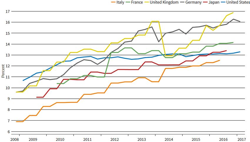
1         Introduction
Financial cycles are less frequent than average business cycles. However, when speculative
financial bubbles burst, their economic consequences are rather persistent (Reinhart and
Rogoff (2011); Brunnermeier and Oehmke (2013)). A financial bubble consists of three
phases: creation of the bubble (potentially triggered by financial innovation), period of
inflation and sudden burst (or implosion). During the boom the price of an asset deviates
from its intrinsic value, i.e. it is not just determined by supply and demand forces; such
deviation features a positive feedback mechanism. In a burst the prices suddenly fall with
negative feedback mechanism, sometimes below the intrinsic value. These interactions can
amplify economic fluctuations and possibly lead to serious financial distress and prolonged
economic disruption.
    In this paper we formalize the processes of bubble creation and asset price inflation to
provide a setting for the analysis of monetary policy and efficacy of regulatory instruments.
In particular, we consider a real (or rational) trigger of the bubble (financial innovation) and
an (irrational or behavioral) extrapolation of past loan growth into the future asset price.
Hence, the size of loan portfolio is not just determined by supply and demand. The loan
size is also linked to expectations of future loan value with a positive feedback mechanism
in the bubble variable coming from the pricing at the loan trading stage.
    The model comprizes of households who consume, work for firms and banks, and invest in
bank shares: they face a deposit in advance constraint which introduces a spillover from the
financial sector into the real economy. The commercial banking sector comprizes of a bank
headquarter and retail branches which interact with households giving out differentiated
loans to households. The “wholesale” unit is responsible for the management of the capital
position of the bank. We allow for interbank transactions (securitization) in the loan market
where resale of loans triggers the build up of the financial bubble. The repackaging of loans
means a higher value as it allows for a mark-to-market of the price expectations through sale.
This also results in a higher level of bank capital. As the amount of outstanding loans are
linked to optimal bank capital, rising equity capital allows to expand further on the amount
of loans. Finally, there is a monetary authority setting interest rates for bank refinancing.
    We consider several policy options (i ) a conventional monetary policy reaction to changes
in overall loans (“leaning against the wind”); (ii ) a macroprudential measure that increases
exogenously the target level of the capital requirement for bank equity and (iii ) an endoge-
nous capital requirement that reacts to the credit-to-GDP gap. The credit-to-GDP gap
(according to the definition by the BIS) is the difference between the credit-to-GDP ratio
and its long-run trend.1 We find that a “leaning against the wind” policy is not very effective
    1
        In the BIS database the credit-to-GDP ratio is total credit to the private non-financial

                                                 1
in reducing the size of financial bubbles while endogenous macroprudential measures, such as
an endogenous rule reacting to the credit-to-GDP-gap, can target (pure) financial bubbles
more effectively than interest rate policy. This result is also in line with the findings by
Galı̀ (2017) who shows that monetary policies that lean against the bubble are potentially
destabilizing and likely to be dominated by inflation targeting policies.
The paper is organized as follows: The first section discusses the motivation and related
literature. Section 2 to 6 describe the model. Section 7 shows quantitative experiments.
Section 8 concludes.
1.1 Motivation
The run-up of financial bubbles followed by financial crashes is a (sadly) frequent phenomena
in modern economies. The building up of the bubble as well as its crash usually sets a
number of amplification mechanisms linked to the presence of financial frictions and spillovers
effects in the real economy (especially in terms of consumption and investment decisions).
Indeed, “procyclicality” is a relevant feature of financial cycles for macroeconomists and
policymaking: hence the focus on business cycle fluctuations and financial crises (Borio et
al. (2001), Danielsson et al. (2004), Kashyap and Stein (2004), Brunnermeier et al. (2009),
Adrian and Shin (2010)).
Figure 1 shows various developments of the credit cycle (measured by credit-to-GDP
gap) in Japan, the U.S. and Europe. For all countries plotted we see sizable swings in this
measure. Credit expansion and contraction has significant effects on the demand side of the
economy, and thus on economic cycles.
Japan faced a very deep crisis in the early 1990s caused by booming real estate and
stock markets leading to the so-called “lost decade” of the 1990s and enduring low growth
during the 2000s. To prick the bubble in real estate and in the stock market, the Bank
of Japan implemented standard conventional policies by raising the official discount rate in
May 1989, from 2.5% to 6.0%. In addition, the Bank of Japan forced the real estate sector to
de-lever by reducing the amount of lending to the real estate sector where several real estate
firms faced bankruptcy, leading to fire sales and a drop in real asset prices. Ultimately, the
drop in real estate prices led to a decrease in the value of the collateral and to an overall
lending decline with a debt overhang problem for the entire banking sector (see, for example,
Hoshi and Kashyap (2004)). Only in very recent years Japan moved from conventional to
macroprudential policies aiming at increasing the minimum Tier1 ratio of capital over risky
assets from 4.5% (2013) to 6% (2017).
sector and captures total borrowing from all domestic and foreign sources as input data
(https://www.bis.org/statistics/c gaps.htm).
2Figure 1: Credit-to-GDP Gap, Quarterly.
(a) United States (b) Japan
(c) Germany (d) United Kingdom
(e) France (f) Italy
Source: BIS
3Figure 2: Tier1 capital to risk weighted assets
Source: IMF
Policy switches to stricter capital requirements can also be observed in the U.S. and
Europe. The coupling low interest rates and financial innovation in the form of mortgage
securitization2 had fueled the U.S. real estate prices bubble and the following burst in 2007
leading to one of the longest and deepest economic downturn in U.S. history (for a summary,
see Brunnermeier et al. (2009) and Brunnermeier and Oehmke (2013)).
More recently the European Union has been dealing with a major sovereign debt crisis
which has been feeding into the financial sector. As also Borio (2012) notes fiscal policy in-
tervention needs extra caution when economic booms and financial booms are coupled. The
reason is that financial booms do not just enhance the balance sheets of financial institutions
(Borio and Drehmann (2009)), they also enhance the fiscal accounts of public governments
(Eschenbach and Schuknecht (2004), BIS (2010, 2012), Borio (2011), Benetrix and Lane
(2011)). As potential output tend to be overestimated the sovereign inadvertently accumu-
lates contingent liabilities. Furthermore, government bonds typically appear as risk neutral
assets especially in the balance sheet of financial intermediaries. As the bubble busts balance
sheet problems appear, especially in the financial sector, because of the dual risk-exposure
coming from private lending and government assets. The response to the financial crises
both in the U.S., Japan and Europe has been a general increase in capital requirement as
2
Alan Greenspan testifying at the Financial Crisis Inquiry Commission in 2010 explained, ”Whether it
was a glut of excess intended saving, or a shortfall of investment intentions, the result was the same: a fall in
global real long-term interest rates and their associated capitalization rates. Asset prices, particularly house
prices, in nearly two dozen countries accordingly moved dramatically higher. U.S. house price gains were
high by historical standards but no more than average compared to other countries.”
4shown in Figure 2.
1.2 Related Literature
There is a growing literature on financial bubbles in macroeconomic models. Brunnermeier
and Oehmke (2013) analyse the amplification mechanisms of rational bubbles. In models
of rational bubbles, agents hold a bubble asset because its price is expected to rise in the
future. The implied explosive nature of the price path in this class of models is consistent
with the observed run-up phases to many financial crises.
Bubbles can emerge in an overlapping generation setting (Galı́ (2014), (2017)). Further-
more, and in contrast with the earlier literature on rational bubbles, the introduction of
nominal rigidities allow the Central Bank to impact on the real interest rate and, through
it, on the magnitude of the bubble.
Bubbles can also arise and survive because of several class of frictions characterising the
underlying economic model. A more recent strand of literature deals with these counterfac-
tual implications by adding borrowing constraints. For example, in the model by Martin
and Ventura (2012), entrepreneurs face financing constraints so they can borrow only a frac-
tion of their future firm value. When such financing constraints are present, bubbles can
have a crowding-in effect, and thus allow the productive set of entrepreneurs to increase
investments.
The control of bubble-burst episodes in the financial sector has triggered a series of
proposals. Benes and Kumhof (2012) analyse in a DSGE setting the implication of the
Chicago Plan. The key feature of this plan was the control of the credit functions in the
banking system by ensuring that the creation of new bank credit can only take place through
earnings that have been retained in the form of government-issued money, but not through
the creation of new deposits by banks. The plan is preventing banks from creating excessive
inside money during credit booms, and then dismantle it during economic downturns, in
order to soften credit cycles.
More recent macroprudential policies try to influence the supply of credit taking a system-
wide approach. In the absence of macroprudential policy the monetary authority reacts to
an adverse change to financial conditions by using the policy rate to affect the refinancing
conditions of financial intermediaries (Blinder et al. (2008), Carlstrom and Fuerst (1997)).
In extreme situations, as when the Central Bank operates at the zero lower bound, interest
rate policy may be complemented by unconventional tools (Bernanke and Reinhard (2004),
Gertler and Karadi (2011), Curdia and Woodford (2010)).
Woodford (2012) and Svensson (2012) analyse the effectiveness of macroprudential pol-
icy along with an interest rate policy. While Woodford finds a complementary role of both,
5Svensson argues in favor of a clear assignment to financial stability and price stability, re-
spectively. Most of macroprudential tools discussed in the literature are targeted at the
bank’s regulatory capital to address potential vulnerabilities on the demand side of credit.3
Studies which raise the importance of supply side features identify, instead, short term debt
refinancing of banks as a major source of vulnerability and financial innovation in the form
of new financial instruments used in the interbank market.4
Endogenous capital requirements (Borio (2012)) have been proposed as a part of macro-
prudential policies. A key element is to address the procyclicality of the financial sector by
building up buffers in good times, when financial vulnerabilities emerge, so as to be able to
drain them in bad times, when financial strain materialises. There are several ways of inter-
vening in this direction, through the design of macroprudential tools. Basel III, for instance,
has designed a countercyclical capital buffer as opposed to “leaning against the wind policy”
and other forms of capital and liquidity standards.5
The approach in this paper is placed in the literature of general equilibrium models with
supply side financial frictions. We consider a model with bank monitoring and inside money
creation features as in Goodfriend and McCallum (2007) with the added feature of interbank
transactions, in the form of securitization in the loan market, where a resale of loans triggers
the build up of the financial bubble. We model the process of bubble creation following
Branch and Evans (2005) assuming that agents act as econometricians when forecasting
and use this bounded rationality on banks when they evaluate the change in loan value.
The repackaging of loans results in a higher value as it allows for marked-to-market of the
bubble through sale. In a financial system where balance sheets are continuously marked-
to-market, asset price changes show up immediately in changes in net worth, and elicit
responses from financial intermediaries who adjust the size of their balance sheets. Hence
marked-to-market leverage is strongly procyclical (Adrian and Shin, 2008 and 2010) as the
loan bubble feeds into bank’s equity values featuring a banking sector transmission through
endogenous bank capital (see also Gerali et al., 2011). In the proposed setup we analyse the
stabilising effects of several policy options: (i ) a conventional monetary policy reaction to
3
Examples for models with limited borrowing capacity of households are Bernanke, Gertler and Gilchrist
(1999) and Kiyotaki and Moore (1997). Corrado and Schuler (2017), among others, analyse the effects of
several macroprudential policy measures in a model with cash-in-advance households in which banks trade
excess funds in the interbank lending market. They conclude that stricter liquidity measures along with
a moderate capital requirement directly limit inside money creation, therefore reducing the severity of a
breakdown in interbank lending.
4
Justiniano et al. (2015), Gertler and Karadi (2011) and Gertler and Kiyotaki (2010) focus on the role
endogenous leverage constraints for banks to trigger credit supply disruptions.
5
If effective macroprudential frameworks were in place, capital and liquidity buffers could be drained to
control the building up of the bubble. But, if the authorities have failed to build up buffers in good times
and financial problems emerge, the challenge is to act directly on financial institutions’ balance sheets (Borio
(2012)).
6changes in overall loans (“leaning against the wind”); (ii ) a macroprudential measure that
increases exogenously the target level of the capital requirement for bank equity and (iii ) an
endogenous capital requirement that reacts to the credit-to-GDP gap.
2 Model Overview
The model comprizes of households who consume, work for firms and in the banking sector,
and invest in bank shares and bonds. There are intermediate and final good producing firms
which together form the production sector. The commercial banks feature a bank headquar-
ter and retail branches which lend to households. We allow for interbank transactions in form
of trades of securitized loan portfolios. We model productivity, i.e. efficiency in loan produc-
tion, and lending constraints in form of equity capital in the financial sector. A relaxation
of financial constraints by looser regulation often stand at the beginning of credit booms
(e.g. the Japan bubble, U.S. subprime boom, lending booms in some Eurozone countries).
Furthermore, new technologies in loan production (IT) and selling (e.g. securitization) allow
for an expansion of loans. Finally, the model includes a monetary authority which sets the
riskless interest rate.
3 Households
There is a mass one of infinitely-lived households with the utility described by
∞
QΨ
t Ψt
X
t
max E0 β log(ct ) + φl log(1 − lts − mst ) + φe log (1)
t=0
Pt
where ct is consumption, lts labor provided to the production sector and mst labor provided
to the banking sector. QΨ t represents the equity price and Ψt the equity investments. φl
reflects the weight of leisure and φe the weight of stock investments in utility. Households
only can acquire consumption goods by spending bank deposits Dt which means that they
have to fulfill a money in advance constraint given by
Pt ct ≤ vDt (2)
7Their budget is described by the following inequality which involves the interest payments
on loans, Lt , and deposits, Dt :
Bt+1 Dt+1 Lt+1 QΨ Bt
ct + + − + t Ψt ≤ wt (lts + mst ) + (1 + RtB ) ... (3)
Pt Pt Pt Pt Pt
Dt Lt QΨ + ΠΨ
... + (1 + RtD ) − (1 + RtL ) + t t
Ψt−1
Pt Pt Pt
Here Bt are savings in government bonds, wt the real wage for production or banking labor,
Pt the price level, and RtD , RtL , and RtB interest rates on the respective assets and liabilities.
ΠΨ
t relates to dividend payments for bank equity.
4 Firms
Production of consumer goods involves two stages with intermediate inputs. The final goods
firm produces a composite good, yt , by combining intermediate goods, yt (i), through a
constant elasticity of substitution (CES) aggregator, i.e.
1
Z 1 1−
yt = yt (i)1− di (4)
0
The profit function of intermediate firm i is given by
ΠFt (i) = yt (i) − wt lt (i) (5)
Intermediate goods are produced by employing labor lt according to the following technology
yt (i) = A1t lt (i)1−α (6)
In (6), A1t is a shock to productivity in goods production, similar to a standard TFP
shock in the real-business- cycle literature, whose mean increase over time at the trend
growth rate of g.
There is a probability of θ that firms are not able to change the price in a given period.
Thus firms setting the price have to solve the following multi-period problem (Calvo (1983)
pricing), i.e.
∞
X
θk Et {Rt,t+k
B
y(i)t+k|t (Pt∗ (i) − MM Ct+k )} = 0 (7)
k=0
with Pt∗ being the optimal price set in period t.
85 Banking Sector
The financial sector comprizes of commercial banks which are active in the traditional bank-
ing business, i.e. handing out credit to households, and which are able to trade loan portfolios
with each other. Thus the bank business involves a loan origination and trading stage. The
loan origination stage combines the loan management technology of Goodfriend and McCal-
lum (2007) with differentiated loan demand as in Gerali et al. (2011).
5.1 Loan origination
There is a mass 1 of commercial banks with a bank headquarter and retail branches.
Bank headquarter
The bank headquarter decides on the interest rate spread given the optimal amount of loans
and the capital structure. The bank headquarter maximizes its profit function,
∞
" 2 #
X Lt Dt κe et
ΠB
t = RtL − RtD − −τ − wt mt , (8)
t=0
Pt Pt 2 Lt
where Lt is the overall loan portfolio, and Dt are the total household bank deposits and et
bank equity. Banks face a quadratic cost related to a deviation from the optimal ratio of
bank equity versus the loan portfolio, the capital requirement ratio τ .
At the headquarter level the individual bank balance sheet constraint has to hold, i.e.
Lt = Dt + et (9)
Bank headquarters also decide on the amount of monitoring work which is remunerated by
the real wage, wt . It is implied by the size of the loan portfolio through following loan
management technology
Lt
= Qt m1−α
t , (10)
Pt
with Qt being the efficiency in loan production, which can be subject to shocks following a
AR(1) process
Qt = ρ3 Qt−1 + 3t (11)
where 3t is an i.i.d. shock. Optimal loan provision gives the external finance premium on
the bank headquarter level, i.e.
2
vwt mt et et
RtL − RtD = − κe −τ . (12)
(1 − α)ct Lt Lt
9Retail banks
Retail banks hand out differentiated loans to households (following the mechanisms a la Ger-
ali et al. (2011)). Deposit demand for transaction purposes triggers demand for loans. Total
loan demand, Lt , and total deposit demand, Dt , are derived from the money in advance
condition.6 The differentiated loan demand function by households reads as
−L
Rt (j)L
Lj,t = Lt (13)
RtL
for all j retail banks with L being the elasticity of substitution between loans from different
retail branches. This results in an effective loan rate of
L
RtL (j) = RL , (14)
L − 1 t
L
where L −1
represents the loan markup.
Profit, Dividends and Retained earnings
Bank profits, ωB,t , are given by the in-period return over equity and monitoring costs, i.e.
2
Lt Dt κe et
ωB,t = RtL − RtD − −τ − wt mt . (15)
Pt Pt 2 Lt
The share of profits, φΨ , which is paid out as dividends is given by
ΠΨ
t = φΨ ωB,t . (16)
The remaining share, (1 − φΨ ), is booked as a profit to the bank’s equity capital et . The law
of motion for bank capital, et , is then
et = (1 − δe )et−1 + φB (QΨ Ψ
t − Qt−1 )Ψ + (1 − φΨ )ωB,t−1 , (17)
where Ψ is the initial stock of bank equity and φB is the pass-through of equity price
changes to bank capital. Stock price changes (QΨ Ψ
t − Qt−1 ) result from changes in profits.
The dying rate of bank capital δe , captures sunk cost of bank capital management. QΨ t Ψ
6
Deposit demand equivalently reads as
−D
Rt (j)D
Dj,t = Dt
RtD
10represents the market capitalization of the bank.
5.2 Loan securitization and trading
Banks are allowed to securitize loans into tradable loan portfolios, and exchange them with
each other with their given value plus a profit.7
Initial financial innovation shock. We assume a financial innovation shock which is a
Figure 3: Shock to loan production efficiency
Rt
LQ
s
low
LsQ high
Rt1
Rt2 Ld1
t
Lt
L1t L2t
productivity shock to the efficiency of the bank loan production function, Qt , by which the
size and thus the value of the loan, Lt , increases at banks. We can think of the productivity
shock to the efficiency in loan production, Qt , as a new technology shock which allows to
increase the loan output while reducing the monitoring need of banks. The mechanism is
illustrated in Fig. 3 which shows the loan demand and loan supply, and the interest rate at
which the market clears. A higher efficiency in loan production allows for an outward shift
in the loan supply curve.
Bubble creation through resale technology. The expectation formation plays a
crucial role for the development of the financial bubble. In this respect we deviate from the
fully informed agent paradigm. Several contributions to the literature support a deviation
from the rational expectations assumption. As Branch and Evans8 (2005) we assume that
7
See Brunnermeier (2009) for a detailed treatment on loan securitization according to the “originate and
distribute model” characterizing bank behavior before the financial crisis of 2007-08 in the US.
8
Branch and Evans (2005) evaluate the effectiveness of different prediction models for economic growth.
They compare four different methods: Recursive Least Squares (RLS), Kalman-filter method, Constant Gain
Least Squares and a special case of Constant Gain Least Squares which allows the constant gain to be equal
for every variable (Simple Method). The Constant Gain Method and specifically the Simple Method turn
out to provide the best results which allows the conclusion that this is a method worth considering with
11Figure 4: Expansion of equity capital due to mark-to-market
Rt
Les high
Rt2 Ld1
t
Lt
L2t
agents act as econometricians when forecasting and implement this bounded rationality on
banks when they evaluate the change in value of loan portfolios. The estimation follows a
Kalman Filter recursion where the banking sector monitors past growth in value of loans,
i.e.
lnLt − lnLt−1 = gt + wt
with wt being a short run fluctuation around gt , the economy’s growth rate. The short run
fluctuation, wt , differs conceptionally from shocks to Qt , the efficiency of loan management.
In their expectation formation process bank agents just monitor past changes in loan value.
They do not consider the contribution of (aggregate) bank productivity measures when they
form expectations about the growth in future value. gt is a AR(1) process around the mean
g, i.e.
gt = (1 − δg )g + δg gt−1 + ηt
where ηt is an i.i.d. shock. The expectation operator of the not-fully informed agent reads
as
Ẽt (lnLt+1 − lnLt ) = Ẽt (gt+1 + wt+1 ) (18)
= Ẽt (1 − δg )g + δg Ẽt gt
where Ẽt is the expectation operator with an adaptive expectation formation. By replacing
the expectation of gt the expression becomes backward looking.9 For the expectation of the
regards to the expectations formation of economic agents that adapt to continuous structural changes in the
economy.
9
Compare to Milani (2005) who examines and tests whether agents in the economy have rational expecta-
12growth trend of the economy, we assume that banks mix between monitoring last period’s
growth trend, gt−1 , and the growth in the value of loans:
Ẽt gt = (1 − κ)δg Ẽt−1 gt−1 + κ(lnLt − lnLt−1 )
with κ being the weight on last period’s growth trend. Replacing this into (18), multiplying
out and collecting terms we derive the expectation of the future loan value:
Ẽt (lnLt+1 ) = (1 − δg )g + δg2 (1 − κ)Ẽt−1 gt−1 + lnLt + δg κ(lnLt − lnLt−1 )
So when banks sell a loan portfolio through securitization they realize gains through expected
future valuation changes, i.e.
Ẽt (lnLt+1 ) = lnLt + ln(bt ) (19)
where we assume δg and κ to be 1. Through the Kalman filter the expectation formation
about future prices depends on the past changes in the value of the loan portfolio:
Lt
bt = (20)
Lt−1
Thus the size of the bubble is determined by extrapolating the pace of loan growth which
makes it backward looking. Using condition (19) and plugging it into the above loan pro-
duction function results in:
Ẽt {Lt+1 } bt
= Qt mt1−α + . (21)
Pt Pt
Transmission to bank equity. The repackaging of loans results in a higher value, with
the bubble term, bt , being the profit of this transaction. The repackaging technology allows
for a mark-to-market of the bubble through sale. This results in a higher level of bank equity
by the bubble size, i.e. et + bt . This is illustrated in Fig. 4. As the amount of outstanding
loans is linked to optimal bank capital, rising equity capital allows the bank headquarter to
expand further on the total amount of loans, Lt , i.e.
et+1 ↑≈ τ Lt+1 ↑ (22)
tions with regards to economic growth or whether it can be assumed that they show learning behaviour. The
latter presumes that agents do not fully know the underlying economic model with all its parameters, so they
forecast the future based on their observed values from previous periods. He finds that the adaptive learning
method helps to improve the fit of the DSGE models. Similarly, Eusepi and Preston (2011) introduce a
model in which agents do not have full knowledge of the economic processes, but predict future realisations
by extrapolation from historical patterns in observed data. This results in a higher volatility and a higher
persistence of macroeconomic variables which corresponds with the observed data.
13Figure 5: Increase in loan demand
Rt
Les high
Rt3
Rt2 Ld2
t
Ld1
t
Lt
L2t L3t
We can separate two cases: first, if equity capital, et , is scarce, then the increase in equity
capital leads to an expansion of loans in the next period, Lt+1 , as the constraint is relaxed
and banks can service more demand for credit. Alternatively, if equity capital is abundant,
loans, Lt+1 , will also expand as banks are able to lower the credit spread along with lower
capital costs. Through this effect we see a spill-over to the demand for credit which shifts
outwards and absorbs the higher lending capacity of banks. This mechanism is illustrated
in Fig. 5.
5.3 Discussion: From the standard model to the bubble model
We incorporate two main features which characterize a bubble into a DSGE model with
banks: First, the size of loan portfolio is not just determined by supply and demand in the
loan market. Instead of just matching consumption through the money in advance condition,
the loan size is also linked to expectations of future loan value, which allows for a bubble
component in pricing. There is a (positive) feedback mechanism in the bubble variable
coming from the pricing at the loan trading stage. The feedback mechanism leads to an
excessive growth of loans over GDP while the bubble is growing. Second, this additional
loan supply through the banking sector keeps consumption higher than given by what a
household could fundamentally afford through its consumption-savings decision.
146 Monetary policy
The policy rate follows a Taylor (1993) rule which reacts to inflation, πt , and fluctuations in
output, yt , i.e.
(1−ρ)φy
p p
ρ πt (1−ρ)φπ yt
Rt = Rt−1 A3t (23)
π∗ yt−1
with A3t following a AR(1) process. We modify the Taylor rule for further experimentation
in the quantitative section.
7 Quantitative Results and Policy Experiments
We solve the model for its equilibrium, calculate non-stochastic steady states and linearize
the model around the steady state. In the following we describe the benchmark calibration
for the simulation of the model, before we show impulse responses for a financial bubble
shock. Finally, we employ the simulated model for several policy experiments.
7.1 Benchmark Calibration
The model is calibrated to quarterly frequencies matching endogenous aggregates and interest
rates to observable data. We assume zero average inflation. The household discount factor
is set to 0.99 implying an annual real rate of interest of 4% for the riskless bond rate RB .
15Table 1. Parameters
β discount factor 0.997
η concavity in production 0.34
α concavity in loan management 0.38
φl weight of leisure in utility 0.7
Dixit-Stiglitz parameter 6
τ equity target level 0.11
v velocity of money 0.31
θ share of firms without price reset 0.77
M price markup 1.2
ML loan rate markup 1.4
φπ weight of inflation in policy function 1.5
φy weight of output in policy function 0.5
ρ smoothing in policy function 0.25
ωΨ share of dividends in bank profits 0.68
δe equity depreciation 0.025
κe leverage deviation cost 4
φB equity price pass-through 0.35
L elasticity loan demand 3.5
The share of intermediate firms which cannot reset their price in a given period is θ = 0.77.
The Dixit-Stiglitz parameter, , is set to 6 generating a mark-up of 20%. The velocity of
money v is set to 0.31 on the basis of average GDP to M3 after the U.S. subprime crisis.
The capital requirement ratio τ is set to 11%. For further experimentation we change τ to
15%. We assume a coefficient equal to 0.34 for the concavity of labor in the the production
function of the intermediate product; for loan management we choose a coefficient of equal
to 0.65.
16Table 2. Implied Steady-States
RP policy rate 0.0084
RB bond rate 0.0101
RD deposit rate 0.0067
RL loan rate 0.0169
c consumption 0.6244
l
c
production work 0.4900
D
c
deposits 2.0145
L
c
loans 2.0145
w wage 0.9588
m
c
monitoring work 0.0246
ωB bank’s profits 0.0239
φΨ share of bank’s profits paid as dividends 0.7690
e equity 0.2215
ΠΨ bank’s dividends 0.0184
QΨ equity price 1.8258
We set total labor supplied in steady state to 1/2 of hours, similar to Goodfriend and
McCallum (2007). The share of working time devoted to banking services is 2%. This implies
that a share of 49% of total time is in the production sector and 1% in the banking sector.
Following Gerali et al. (2011) we calibrate the banking parameters to replicate data averages
for commercial bank interest rates and spreads. We calibrate the steady states to RB = 4%
p.a. and RIB = 3.36% p.a. This implies an annualized return for RD = 2.6% p.a. and a
loan rate RL = 6.7% p.a. From the derivation of the implied steady states of the model we
have that 76% of profits are paid as dividends assuming that equity depreciates at 10% p.a..
Table 3. Calibration of exogenous shocks
Persistence
ρ1 productivity 0.95
ρ2 monetary policy 0.9
ρ3 financial innovation 0.9
Volatility
σ1 productivity 0.72%
σ2 monetary policy 0.82%
σ3 financial innovation 1%
The technology shocks are assumed to be quite persistent, with a standard deviation
equal to 0.72% and an autoregressive parameter 0.95. The shock to the policy rate has a
17standard deviation equal to 0.82%, and an autoregressive parameter of 0.9, and for the fi-
nancial innovation shock we assume a higher standard deviation of 1% and an autoregressive
parameter equal to 0.9. Shocks to the TFP have a relatively prolonged effect on macroeco-
nomic variables, while a monetary policy shock rapidly dies out and the economy reaches
again the steady state. The bubble shock is modeled as being somewhat persistent due to
its effects on loan creation. Monetary policy coefficients on inflation and the output are 1.5
and 0.5. The rest of the parameters, implied steady states and interest rates used in the
calibration are given in Tables 1-3.
Figure 6: Impulse responses to a financial bubble shock
Note: All interest rates are shown as absolute deviations from the steady state, expressed in
percentage points. All other variables are percentage points deviations from the implied steady
state value.
7.2 Impulse response for the Financial Bubble
We first show the impulse response to a financial innovation shock in Fig. 6 and then the
impulse under a variation of price persistence.
The financial innovation shock leads to a reduction in monitoring needs to service given
transaction money demand. Simultaneously, the bank spread (external finance premium, or
18EFP) and the equity price are lowered. The amount of loans handed out by banks rise on
impact. Then they further increase due to the positive feedback mechanism of the financial
bubble. The financial bubble has a direct impact on inflation and due to staggered pricing
also real effects on consumption in addition to the initial financial innovation shock.
We illustrate the effect of the staggered pricing mechanism (as in Calvo (1983)) under the
financial bubble shock (Fig. 7). We find that with higher price persistence less adjustment
is channeled through inflation and real effects are higher. Hence, the effects of a financial
bubble differ for economies depending on the degree of price flexibility. In particular, the
assumption of sticky prices makes monetary policy non-neutral, allowing it to influence the
size of the bubble; on the other hand, price stickiness makes it possible for aggregate bubble
fluctuations to influence aggregate demand and, hence, output and employment.
Figure 7: Impulse responses to a financial bubble shock with high and low price inertia
Note: All interest rates are shown as absolute deviations from the steady state, expressed in
percentage points. All other variables are percentage points deviations from the implied steady
state value.
197.3 Policy experiments
We test how effective several monetary and macroprudential policies are in this setup:
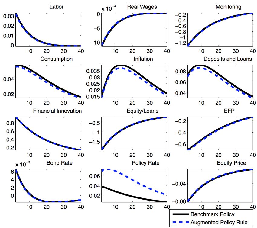
In Fig. 8 we study the effect of monetary policy reacting to changes in overall loans, Lt .
This would modify the Taylor rule of the monetary authority towards
φL (1−ρ) (1−ρ)φy
ρ Lt πt (1−ρ)φπ yt
Rtp = p
Rt−1 A3t . (24)
L π∗ yt−1
We see in the impulse response that the modified Taylor rule has little effect on inflation
and consumption although the policy reaction doubles. A reaction to overall loan growth
barely affects bank leverage, the credit margin (EFP) or the equity price. We conclude that
a “leaning against the wind” policy is not effective in reducing the size of financial bubbles.
Figure 8: Impulse response with different monetary policy reaction
Note: All interest rates are shown as absolute deviations from the steady state, expressed in
percentage points. All other variables are percentage points deviations from the implied steady
state value.
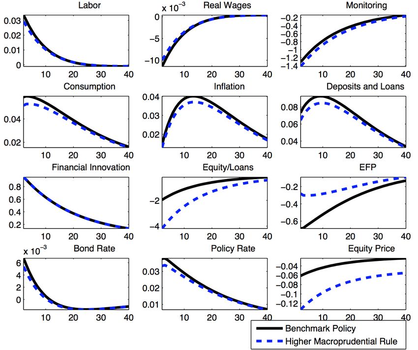
The next experiment uses a macroprudential measure by increasing the target level of
20the capital requirement ratio, τ , from a level of 11% towards 15%.
∞
" 2 #
X Lt Dt κe et
ΠB
t = RtL − RtD − −τ − wt mt (25)
t=0
Pt Pt 2 Lt
The increased capital requirement ratio leads to a reduction of the impact of the shock
as demonstrated in Fig. 9. The response of inflation and consumption is dampened. This
works through the equity price which is lowered during a financial shock (almost twice as
much compared to the base case). On the other hand, the negative impact on the spread
between the loan and deposit rate is reduced, meaning that the financial sector can better
absorb the bubble shock.
Figure 9: Impulse response with higher equity requirement
Note: All interest rates are shown as absolute deviations from the steady state, expressed in
percentage points. All other variables are percentage points deviations from the implied steady
state value.
Finally, in Fig. 10 we introduce an endogenous capital requirement, τt , set by regulator
along the following rule reacting to the credit-to-GDP gap:
21
                                                      Lt   L
                                    τt = τ + κt          −                                   (26)
                                                      Yt   Y

                 Figure 10: Impulse response with endogenous requirement

  Note: All interest rates are shown as absolute deviations from the steady state, expressed in
 percentage points. All other variables are percentage points deviations from the implied steady
                                          state value.

    Under the rule reacting to the credit-to-GDP gap we see a reaction of the financial bubble
compared to the base case. While the equity price falls more than in the base case (but less
than under the exogenous increase in target capital), the reaction of the spread (external
finance premium, EFP) is much lower. The stabilization comes from the combination of
a lower equity price and a smaller response of deposits and loans. The side effects of the
financial bubble are reduced, inflation and consumption react significantly less. The visible
impact on the target variables inflation and consumption while at the same time other
variables do not move let us conclude that an endogenous requirement is effective in precisely
working in the required way without adversely affecting other macroeconomic variables.
    Supporting this reasoning, Table 4 shows that under and endogenous macroprudential

                                               22
rule the volatility of consumption and loans is sensibly attenuated while the volatility of
equity and equity prices increases.
Table 4. Model Moments
Benchmark Endogenous Capital Requirement
S.D. Corr. S.D. Corr.
Consumption 0.1638 1 0.1078 1
Equity 2.72132 0.5188 6.7513 0.2133
Equity Prices 0.08529 0.4408 0.2185 0.1688
Loans 0.4477 0.9711 0.3326 0.7545
8 Conclusions
In this paper we set up a framework for the causes and effects of a financial bubble. With this
model we shed light on recent policy debates on monetary and macroprudential instruments.
The financial bubble features the deviation of the value of an asset from its equilibrium
value determined by supply and demand, as well as a positive feedback mechanism for the
value deviation. The analytical framework shows how a financial bubble can develop from the
bank supply side with households following standard behavioral functions. We demonstrate
how a bubble in the banking sector relaxes financing constraints on the liability side as it
increases the value on the asset side of bank balance sheets. Through higher bank lending,
the financial bubble generates (temporary) income effects at the side of the households.
We test several measures on whether they can effectively reduce the impact of a financial
bubble. We find that a macroprudential rule which reacts to the credit-to-GDP gap proves to
be the most effective measure to prevent a bubble from growing. A central bank intervention
against the financial bubble (“leaning against the wind”) has only a minor effect. We thereby
provide a rationale for the use of counter-cyclical capital buffers.
23References
[1] Adrian T. and H.S. Shin (2008): Procyclical Leverage and Value at Risk, Federal Reserve
Bank NY Staff Report 338.
[2] Adrian, T. and H.S. Shin (2010): Liquidity and Leverage, Journal of Financial Inter-
mediation, 19(3), 418-437.
[3] Benes, J. and M. Kumhof (2012): From Financial Crash to Debt Crisis, IMF Working
Paper ,P/12/202.
[4] Benetrix, A. and P. Lane (2012): The Cyclical Conduct of Irish Fiscal Policy, The
World Economy, 35(10), 1277-1290.
[5] Bernanke, B, M. Gertler and S. Gilchrist (1999): The Financial Accelerator in a Quan-
titative Business Cycle Framework, in J Taylor and M Woodford (eds), Handbook of
Macroeconomics, Amsterdam, 1341-393.
[6] Bernanke, B. S. and V. Reinhart (2004): Conducting Monetary Policy at Very Low
Short-term Interest Rates. American Economic Review, Papers and Proceedings, 94
(2), 85-90.
[7] BIS (2010): Macro-prudential Instruments and Frameworks: A Stocktaking of Issues
and Experiences, Committee on the Global Financial System.
[8] BIS (2012): 82nd BIS Annual Report, June.
[9] Blinder, A., Ehrmann, M., Fratzscher, M., De Haan, J. and D.J. Jansen (2008): Central
Bank Communication and Monetary Policy: A Survey of Theory and Evidence, ECB
WP 0898.
[10] Borio, C., Furfine, C. and P. Lowe (2001): Procyclicality of the financial system and
financial stability: issues and policy options, BIS Working Papers, 1.
[11] Borio, C. and M. Drehmann (2009): Assessing the Risk of Banking Crises – Revisited,
BIS Quarterly Review, March, 29-46.
[12] Borio, C. (2011): Central Banking Post-crisis: What Compass for Uncharted Waters?
in C. Jones and R. Pringle (eds) The Future of Central Banking, Central Banking
Publications. Also available, in slightly extended form, as BIS Working Papers, no 353,
September.
24[13] Borio, C. (2012): The Financial Cycle and Macroeconomics: What Have We Learnt?,
BIS Working Papers, 395.
[14] Branch, W. and G. Evans (2005): A Simple Recursive Forecasting Model, Economic
Letters, Elsevier, 91(2), 158-166.
Brunnermeier, M. (2009): Deciphering the Liquidity and Credit Crunch 2007âe”2008,.
Journal of Economic Perspectives 23(1), 77-100.
[15] Brunnermeier, M., Crocket, A. Goodhart, C., Persaud, A.D. and H.S. Shin (2009):
Fundamental Principles of Financial Regulation, 11th Geneva Report on the World
Economy.
[16] Brunnermeier, M. and M. Oehmke (2013): Bubbles, Financial Crises, and Systemic
Risk, Handbook of the Economics of Finance, Amsterdam: Elsevier.
[17] Calvo, G.A. (1983): Staggered prices in a utility-maximizing framework. Journal of
Monetary Economics 12, 383-398.
[18] Carlstrom, C., and T. Fuerst (1997): Agency Costs, Net Worth, and Business Fluc-
tuations: A Computable General Equilibrium Analysis, American Economic Review,
87(5), 893-910.
[19] Corrado, L. and T. Schuler (2017): Interbank Market Failure and Macro-prudential
Policies, Journal of Financial Stability, 33, 133-149.
[20] Curdia, V. and M. Woodford (2010): Credit Spreads and Monetary Policy. Journal of
Money, Credit and Banking, 42(1), 3-35.
[21] Danielsson, J., Shin, H. and J. Zigrand (2004): The Impact of Risk Regulation on Price
Dynamics, Journal of Banking and Finance, 28(5), 1069-1087.
[22] Eschenbach, F. and L. Schuknecht (2004): Budgetary Risks from Real Estate and Stock
Markets, Economic Policy, 19(39), 313-346.
[23] Eusepi, S. and B. Preston (2011): Expectations, Learning and Business Cycle Fluctua-
tions , American Economic Review, 101 (6), 2844-2872 .
[24] Galı́, J. (2014): Monetary Policy and Rational Asset Price Bubbles, American Economic
Review, 104(3), 721-752.
[25] Galı́, J. (2017): Monetary Policy and Bubbles in a New Keynesian Model with Over-
lapping Generations, Working Paper, CREI
25[26] Gerali, A., S. Neri, L. Sessa and F.M. Signoretti (2010): Credit and Banking in a DSGE
Model of the Euro Area, Journal of Money, Credit and Banking, 42 (s1), 107-141.
[27] Gertler, M., and N. Kiyotaki (2010): Financial Intermediation and Credit Policy in
Business Cycle Analysis. NYU and Princeton.
[28] Gertler, M., and P. Karadi (2011): A Model of Unconventional Monetary Policy, Journal
of Monetary Economics, 58(1), 17-34.
[29] Goodfriend, M., and B.T. McCallum (2007). Banking and Interest Rates in Monetary
Policy analysis: A Quantitative Exploration, Journal of Monetary Economics, 54, 1480-
1507.
[30] Justiniano, A., G. E. Primiceri, and A. Tambalotti (2015): Credit Supply and the
Housing Boom. Federal Reserve Bank of New York Staff Reports, 709, February 2015.
[31] Hoshi, T. and A. Kashyap (2004): Japan’s Financial Crisis and Economic Stagnation,
Journal of Economic Perspectives, 18(1), 3-26.
[32] Kashyap, A. and J. Stein (2004): Cyclical Implicatons of the Basel II Capital Standards,
Economic Perspectives, 28, 18-31.
[33] Milani, F. (2005): Expectations, Learning and Macroeconomic Persistence , Journal of
Monetary Economics, 54 (7), 2065-2082.
[34] Martin, A., and J. Ventura (2012): Economic Growth with Bubbles, American Eco-
nomic Review, 147(2), 738-758.
[35] Reinhart, C. and K. Rogoff, (2011): From Financial Crash to Debt Crisis, American
Economic Review, 101(5), 1676-1706.
[36] Svensson, L. E. O. (2012): Central-banking Challenges for the Riksbank: Monetary Pol-
icy, Financial-stability Policy and Asset Management. CEPR Discussion Papers 8789.
[37] Taylor, J. B. (1993): Discretion versus Policy Rules in Practice. Carnegie-Rochester
Conference Series on Public Policy, 39 195-214.
[38] Woodford, M. (2012): Inflation Targeting and Financial Stability, Sveriges Riksbank
Economic Review, 1, 7-32.
26A Linearised model
Let x
b denote the deviation of a variable x from its steady state. The model can then be
reduced to the following linearised system of equations:
1) Supply of production and monitoring labor
l m
λ
bt + w
bt = lt +
b m
bt (27)
1−l−m 1−l−m
2) Demand for production labor
bt = −ηb
w lt + a1t (28)
3) Monitoring demand
1b
ct + LRL L
λt + cb btL + LRD L
bt + R btD = 0
bt − R (29)
λ
4) Production
ct = (1 − η) b
b lt + a1t (30)
5) Supply of banking services
ct = (1 − α) m
b b t + a2t (31)
6) Money in advance constraint
ct + Pbt = D
b bt (32)
7) Inflation
bt = Pbt − Pbt−1
π (33)
8) Calvo (1983) pricing
π
bt = βEt π
bt+1 + ϑmc
ct (34)
with ϑ = (1−θ)(1−βθ)
θ
1−η
1−η+η
9) Marginal cost
1
mc bt −
ct = w ct ) + (1 − η) b
(ηb lt (35)
1−η
10) Bond holding
27B
bt = 0 (36)
11) Stock holding
Ψ̂ = 0 (37)
12) Loans
L
bt = D
bt (38)
13) Equity
e(1 − δe )b
et−1 − eb bΨ − Q
et + φB Q(Q bΨ )Ψ + (1 − φΨ )ωB ω
bB,t−1 (39)
t t−1
14) Bond rate
bB = π
R bt − Et λ
bt + λ bt+1 (40)
t
15) Equity price
bt+1 + QΨ Q
Et λλ b Ψ + ΠΨ Π
bΨ − π t+1 − λ λ
b t + Q Ψ bΨ
Q =0 (41)
t+1 t+1 b t
16) Loan spread
" #
vwt mt
L RD RtD + (ŵt + m̂t − ĉt )
RL RtL = (1−α)c
(42)
L − 1 − κLe2e 2 L − τ ebt − κLe2e 3 Le − 2τ L
e
bt
17) Deposit rate
bD = R
R bP (43)
t t
18) Policy feedback rule
bP = (1 − ρ) (φπ π
R bt + φcb bP + a3t
ct ) + ρR (44)
t t−1
19) Bank Profit
L L D D
ωB ω
bB,t = R L Rt + Lt − R L Rt + Dt −
b b b b (45)
κe e e
− τ ebt − L
bt − wm (wbt + m
b t)
L L
20) Dividends:
28bΨ = ω
Π bB (46)
t
21) EFP:
ef p ef pt = RL R
b L − RD R
t
bD
t (47)
There are 21 equations and 21 variables.
B Calculating Steady States
There is no technological progress A1t = A1 = 1 and no price change i.e. Pt = P = 1.
1
1 + RB = (48)
β
RD
RD = (1 − rr) RP (49)
RL
vwm
R = χL RD +
L
(50)
(1 − α)c
c
c = A1l1−η (51)
D
c
D= (52)
v
w
w = (1 − η) l−η (53)
L
L=D (54)
m
1
1−α
L
m= (55)
Q
λ
29φl
λ= (56)
w(1 − l − m)
ωB
ωB = RL − RD L − wm
(57)
φΨ
(1 − φΨ )
e = ωB (58)
δe
e (1 − φΨ ) ωB
τ = =
L δe L
τ δe L = ωB − φΨ ωB
τ δe L
φΨ = 1 −
ωB
e
(1 − φΨ )
e= ωB (59)
δe
ΠΨ
ΠΨ = φΨ ωB (60)
QΨ
QΨ + Π Ψ
1 = βEt (61)
QΨ
Ψ βΠΨ
Q =
(1 − β)
RL − RD
RD
L D L vwt mt
R −R = + (62)
L − 1 L − 1 (1 − α)c
30ifo Working Papers
No. 259 Löffler, M., A. Peichl and S. Siegloch The Sensitivity of Structural Labor Supply Estima-
tions to Modeling Assumptions, March 2018.
No. 258 Fritzsche, C. and L. Vandrei, Causes of Vacancies in the Housing Market – A Literature
Review, March 2018.
No. 257 Potrafke, N. and F. Rösel, Opening Hours of Polling Stations and Voter Turnout:
Evidence from a Natural Experiment, February 2018.
No. 256 Hener, T. and T. Wilson, Marital Age Gaps and Educational Homogamy – Evidence
from a Compulsory Schooling Reform in the UK, February 2018.
No. 255 Hayo, B. and F. Neumeier, Households’ Inflation Perceptions and Expectations:
Survey Evidence from New Zealand, February 2018.
No. 254 Kauder, B., N. Potrafke and H. Ursprung, Behavioral determinants of proclaimed sup-
port for environment protection policies, February 2018.
No. 253 Wohlrabe, K., L. Bornmann, S. Gralka und F. de Moya Anegon, Wie effizient forschen
Universitäten in Deutschland, deren Zukunftskonzepte im Rahmen der Exzellenziniti-
ative ausgezeichnet wurden? Ein empirischer Vergleich von Input- und Output-Daten,
Februar 2018.
No. 252 Brunori, P., P. Hufe and D.G. Mahler, The Roots of Inequality: Estimating Inequality of
Opportunity from Regression Trees, January 2018.
No. 251 Barrios, S., M. Dolls, A. Maftei, A. Peichl, S. Riscado, J. Varga and C. Wittneben, Dynamic
scoring of tax reforms in the European Union, January 2018.
No. 250 Felbermayr, G., J. Gröschl and I. Heiland, Undoing Europe in a New Quantitative Trade
Model, January 2018.No. 249 Fritzsche, C., Analyzing the Efficiency of County Road Provision – Evidence from Eastern
German Counties, January 2018.
No. 248 Fuest, C. and S. Sultan, How will Brexit affect Tax Competition and Tax Harmonization?
The Role of Discriminatory Taxation, January 2018.
No. 247 Dorn, F., C. Fuest and N. Potrafke, Globalization and Income Inequality Revisited,
January 2018.
No. 246 Dorn, F. and C. Schinke, Top Income Shares in OECD Countries: The Role of Govern-
ment Ideology and Globalization, January 2018.
No. 245 Burmann, M., M. Drometer and R. Méango, The Political Economy of European Asylum
Policies, December 2017.
No. 244 Edo, A., Y. Giesing, J. Öztunc and P. Poutvaara, Immigration and Electoral Support for
the Far Left and the Far Right, December 2017.
No. 243 Enzi, B., The Effect of Pre-Service Cognitive and Pedagogical Teacher Skills on
Student Achievement Gains: Evidence from German Entry Screening Exams,
December 2017.
No. 242 Doerrenberg, P. and A. Peichl, Tax morale and the role of social norms and reciprocity.
Evidence from a randomized survey experiment, November 2017.
No. 241 Fuest, C., A. Peichl and S. Siegloch, Do Higher Corporate Taxes Reduce Wages? Micro
Evidence from Germany, September 2017.
No. 240 Ochsner, C., Dismantled once, diverged forever? A quasi-natural experiment of Red
Army misdeeds in post-WWII Europe, August 2017.
No. 239 Drometer, M. and R. Méango, Electoral Cycles, Effects and U.S. Naturalization Policies,
August 2017.
No. 238 Sen, S. and M.-T. von Schickfus, Will Assets be Stranded or Bailed Out? Expectations of
Investors in the Face of Climate Policy, August 2017.You can also read