Working Paper Series Stress-testing net trading income: the case of European banks - European Central Bank
←
→
Page content transcription
If your browser does not render page correctly, please read the page content below

Working Paper Series
 Carla Giglio, Frances Shaw, Nicolas Syrichas,   Stress-testing net trading income:
                         Giuseppe Cappelletti
                                                 the case of European banks

                                                   No 2525 / February 2021

Disclaimer: This paper should not be reported as representing the views of the European Central Bank
(ECB). The views expressed are those of the authors and do not necessarily reflect those of the ECB.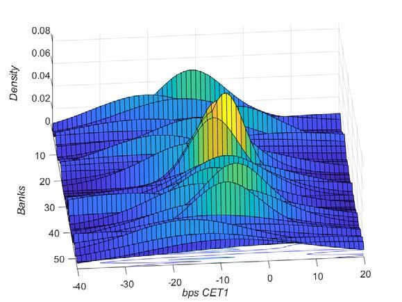
Abstract
          Net trading income is an important but volatile source of income for many euro
      area banks, highly sensitive to changes in financial market conditions. Using a repre-
      sentative sample of European banks, we study the distribution of net trading income
      (normalized by total assets) conditional to changes in key macro-financial risk factors.
      To map the linkages of net trading income with financial risk factors and capture non-
      linear effects, we implement a dynamic fixed effects quantile model using the method
      of moments approach. We use the model to empirically estimate and forecast the con-
      ditional net trading income distribution from which we quantify tail risk measures and
      expected losses across banks. We find a heterogeneous and asymmetric impact of the
      risk factors on the distribution of net trading income. Credit and interest rate spreads
      affect lower quantiles of the net trading income distribution while stock returns are
      an important determinant of the upper quantiles. We also find that the onset of the
      Covid-19 pandemic resulted in a significant increase in the 5th and 10th percentile ex-
      pected capital shortfall. Moreover, adverse scenario forecasts show a wide dispersion of
      losses and a long-left tail is evident especially in the most severe scenarios. Our findings
      highlight strong inter-linkages between financial risk factors and trading income and
      suggest that this tractable methodology is ideal for use as an additional tool in stress
      test exercises.

Keywords: Stress testing, net trading income, quantile panel regression, capital shortfall

JEL Codes: C21, C23, G21, G28

ECB Working Paper Series No 2525 / February 2021                                                     1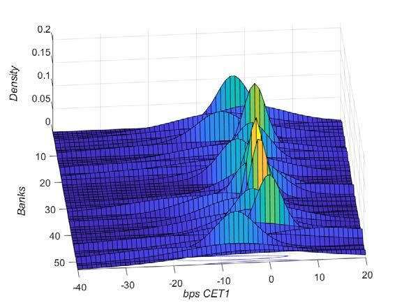
Non-Technical Summary

   Since 2014, a large share of banks’ net operating income in the euro area arises from

non-interest income activities where net fee and commission income (NFCI) and net trading

income (NTI) are the most important contributors. Diversification of income sources can

have unintended consequences, it can create new risks and challenges for the banking sector.

   From a regulatory and supervisory perspective, quantifying and modelling of these bal-

ance sheet items’ evolution in a stress scenario remains a relevant and unmet need. Modelling

non-interest related sources for stress-test purposes is not straightforward as the source of

risks and the channel of transmission might differ from the one already investigated in the

literature. For instance, trading income is likely to be much more volatile and responsive to

financial developments while credit risk is related to slow moving macro variables.

   This paper seeks to fill this void by empirically estimating the linkages between financial

risk factors and net trading income. We focus on net trading income as it is the most volatile

and riskiest of all the non-interest income activities. We find a strong and asymmetric

impact of the risk factors on the tails of the distribution of NTI over total assets (NTI/TA).

In particular, long term interest rates, credit spreads and oil returns exhibit a strong positive

effect on the lower quantiles of the NTI/TA distribution, an effect that dissipates over higher

quantiles. On the other hand, stock returns have a significant (positive) effect only on the

right tail of the NTI/TA distribution. We also find that bank specific characteristics such

as the amount of risk weighted assets and the total equity the bank hold is a poor indicator

of NTI/TA performance across quantiles.

   The volatile nature of trading income can lead to increased downside tail risk, that is,

the risk that a bank experiences an extreme trading loss. Extreme returns cause “fatter”

tails than a normal distribution would predict. Inter-linkages between financial risk factors

and trading income indicate that financial crisis and adverse market shocks can produce left

tail events which could have a damaging impact on the trading portfolio. We employ the

estimated cumulative distribution function to gauge the (time-varying) conditional expected

shortfall of capital at different time horizons and across banks. Using expected capital short-

fall (see Acharya at al., 2012) we can quantify the tail risk as the expected loss conditional

ECB Working Paper Series No 2525 / February 2021                                               2
on the bank experiencing an extreme event (a loss greater than the 5th or 10th percentile

for example). We find that at the onset of the Covid-19 pandemic the expected CET1 ratio

shortfall due to trading income losses at the 5th percentile ranges between -15 and -100

basis points with all banks exceeding what could be considered a material loss.

   One of the objectives of stress-test models is to forecast of banks’ balance-sheet items

under different hypothetical stress scenarios. The severity of the stress scenarios is directly

related to the realizations of the market risk factors. In this respect, our stress scenarios

can be calibrated to the respective quantiles of the risk factors giving a clear and intuitive

interpretation of the scenario and the implied loss distribution. We use the model to deliver

multi-steps forecasts of NTI/TA for banks for various quantiles that reflect different degree

in the severity of the scenario.

ECB Working Paper Series No 2525 / February 2021                                              3
1     Introduction

In recent years, a growing literature emerged on the importance, design and implications

of stress-tests as a tool to assess the resilience of the financial system (V. Acharya, En-

gle, and Richardson (2012); Covas, Rump, and Zakrajšek (2014); V. Acharya, Engle, and

Pierret (2014); Coffinet, Lin, and Martin (2009); Lehmann, Manz, et al. (2006); Albertazzi

and Gambacorta (2009); Schuermann (2014)). Most of the contributions quantify the im-

pact of adverse macroeconomic scenarios in terms of capital shortfall, risk weighted assets

(V. Acharya, Engle, and Pierret (2014), V. Acharya, Engle, and Richardson (2012)) or the

most relevant source of bank’s revenue - net-interest income (V. V. Acharya, Berger, and

Roman (2018)). However, market deregulation and the protracted period of low interest

rates in the aftermath of the 2007-09 financial crisis induced banks to diversify away from

interest-related earnings. In the euro area, around 40%1 of banks overall net operating

income arises from non-interest income23 activities with net fee and commission income

(NFCI) and net trading income (NTI) to be the most important4 .

    The increasing importance of NTI and NFCI can contribute to foster diversification in

banks’ income sources (Stiroh (2004)), it can set new risks and challenges for the banking

sector (Lepetit et al. (2008)). Very recently, numerous researchers documented that non-

interest income and systemic risk are highly positively correlated (Brunnermeier, Dong,

and Palia (2020), De Jonghe (2010) and Moore and Zhou (2014), and Bostandzic and

Weiss (2018)). From a regulatory and supervisory perspective, quantifying the evolution of

these balance sheet items in a stress scenario remains a relevant and unmet need. Modelling

non-interest related sources for stress-test purposes is not straight forward as the source of

risks and the channel of transmission might differ from the one already investigated in the

literature. For instance, trading income is likely to be much more volatile and responsive to
   1 Stiroh (2004) shows that the share of non-interest income over net operating revenue (i.e. net interest

income plus net non-interest income) increased from 25% in 1984 to 43% in 2001 for US commercial banks.
Bank (2000) reports that non-interest income as a percentage of operating income has increased from 32%
to 41% for European banks between 1995 and 1998.
   2 see Figure A.11 in Appendix
   3 By non-interest income, we mean net non-interest income, which is defined as total non-interest income

less total non-interest expense. It refers to brokerage fees, commissions, income from trading activities,
securitization, investment banking.
   4 In the US net-interest income is also around 40% (DeYoung and Rice (2004))

ECB Working Paper Series No 2525 / February 2021                                                          4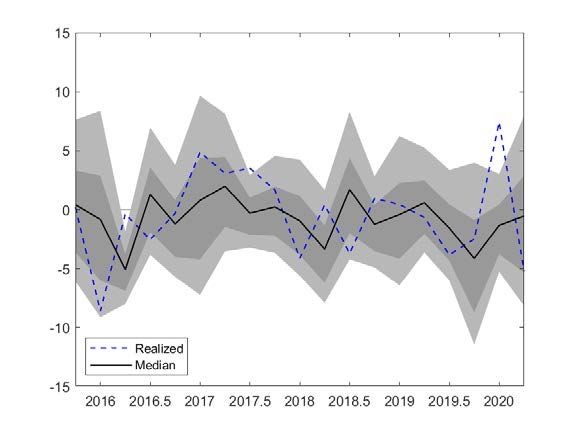
financial developments while credit risk is related to slow moving macro variables. NTI is

an important element of the Market Risk framework in the EU-wide stress-testing exercise.

Every two years the European Banking Authority (EBA) carries out EU-wide stress tests

in cooperation with the European Central Bank (ECB), the European Systemic Risk Board

(ESRB) and the national supervisory authorities. The sample included in the test covers

the largest significant banks supervised directly by the ECB. The exercise uses the EBA’s

methodology and templates, and the scenarios and key assumptions are developed jointly

between the EBA, the ESRB, the ECB and the European Commission. Both aggregate

and individual results are published by the EBA. In the current methodology, banks project

their trading income for 3 years ahead taking into account the impact of the adverse market

risk scenario on their income generating process.5 .

    This paper seeks to fill this gap in literature by empirically estimating the linkages be-

tween financial risk factors and net trading income. We focus on net trading income as

it is the most volatile and therefore the riskiest6 of all the non-interest income activities.

Our econometric strategy follows a three-step procedure. First we map net trading income

as a share of Total Assets (NTI/TA) jointly with bank specific controls and key financial

risk factors through the lens of a fixed effects quantile regression model. We estimate the

quantile panel model semi-parametrically using the method of moments approach proposed

by Machado and Silva (2019). Next, we use this model to derive the empirical conditional

cumulative distribution function of NTI/TA. We use the empirical conditional distribution

to estimate tail risk measures such as expected capital shortfall and loss probability across

banks. Finally, we employ the model to perform a series of multi-step ahead density fore-

casts.

    We use a sample of significant banks under the direct supervision of the Single Supervi-
   5 Inthe aftermath of the great recession, national authorities have established a series various of stress
test exercises to assess the ability of individual financial institutions to absorb losses and maintain sufficient
capital levels in adverse economic conditions. In the EU, in line with the Capital Requirements Directive
(CRD) and Capital Requirements Regulation (CRR) stress tests were first introduced in 2014 and since
then are carried out every two years on a sample covering broadly 70% of the euro area, each non-euro area
EU Member State and Norway, as expressed in terms of total consolidated assets. See EBA methodological
note (2020)
   6 Given the high volatility, unexpected losses can be generated frequently if appropriate volatility hedging

strategies are not in place

ECB Working Paper Series No 2525 / February 2021                                                                5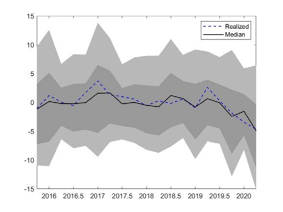
sory Mechanism (SSM). Our sample is at a quarterly frequency and spans over the period

from the fourth quarter of 2014 up to the first quarter of 2020. We consider risk factors to

cover all potential sources of risk for trading income: interest rate risk, credit risk, volatility

risk, exchange rate risk, commodity price risk and equity price risk.7 We find a strong and

asymmetric impact of these risk factors on the tails of the distribution of NTI/TA. In par-

ticular, long term interest rate, credit spreads and oil returns exhibit a strong positive effect

on the lower quantiles of the NTI/TA distribution that dissipates over higher quantiles. On

the other hand, stock returns have a significant (positive) effect only on the right tail of the

NTI/TA distribution. By construction all these effects will not be captured in typical OLS

panel model. We find that bank-specific characteristics such as the amount of risk-weighted

assets and the total equity the banks hold are a poor indicator of NTI/TA performance

across quantiles. This finding suggests that banks’ individual time-varying characteristics

do not matter for trading activities.

    Next, based on the proposed model, we perform a series of pseudo stress tests. Based

on these hypothetical exercises we show that the volatile nature of trading income can lead

to increased downside tail risk, that is, the risk that a bank experiences an extreme trading

loss. Extreme returns cause “fatter” tails than a normal distribution would predict. Inter-

linkages between financial risk factors and trading income indicate that financial crisis and

adverse market shocks can produce left tail events which could have a damaging impact on

the trading portfolio of banks. We employ the estimated cumulative distribution function to

gauge the (time-varying) conditional expected shortfall in terms of capital at different time

horizons and across banks. Using expected capital shortfall we can quantify the tail risk as

the expected loss conditional on the bank experiencing an extreme event (a loss greater than

the 5th or 10th percentile for example). We find that at the onset of the Covid-19 pandemic

the expected CET1 ratio8 shortfall due to trading income losses at the 5th percentile ranges

between -15 and -100 basis points with all banks exceeding what would be considered a

material loss. At the 10th percentile, 43 of 54 banks exceed 15 bps of total risk weighted
   7 The risk factors are: the spread between long and short euro area swap rates, the credit spread between

BBB corporate bond and euro area swap rate, Brent oil returns, major equity indices returns, the VStoxx
index and the return of Euro/US exchange rate.
   8 Common Equity Tier 1 ratio is the ratio of CET1 on risk-weighted assets.

ECB Working Paper Series No 2525 / February 2021                                                          6
assets. We also compute the probability of each bank exceeding net trading income losses of 15 basis points as a share of risk weighted assets. We find that the median probability at the first quarter of 2020 is above 30% across the sample and ranges between 10% and 60% . One of the objectives of stress-test models is to forecast of banks’ balance-sheet items under different hypothetical stress scenarios. The severity of the stress scenarios is directly related to the realizations of the market risk factors. We use the proposed model to deliver multi-steps forecasts of NTI/TA for banks for various quantiles that is related to the degree in the severity of the scenario. This paper is related to two main strands of literature. First it relates to the stress-test literature assessing banks resilience to adverse macroeconomic scenarios (e.g. Quagliariello et al. (2004); Coffinet, Lin, and Martin (2009); Lehmann, Manz, et al. (2006); Albertazzi and Gambacorta (2009)). Most of the papers quantify interest income losses in adverse scenarios. One exception is the study by Coffinet, Lin, and Martin (2009) in which they additionally investigate the effect of adverse shocks on other sources of income, such as commissions, fees and trading activities. The drawback of this type of study is that they rely on standard OLS techniques that might fail to capture the potential non-linear effects of risk factors which is a key feature experienced in the data. Second, we also relate to the literature on the distributional effects of tail shocks. In this respect, many researchers have employed quantile regression techniques. Ghysels, Guérin, and Marcellino (2014) and Schmidt and Zhu (2016) study the distribution of stock returns. Adrian, Boyarchenko, and Giannone (2019) and Figueres and Jarociński (2020) study the GDP growth of US and Euro Area respectively. Chavleishvili and Manganelli (2019) employ a quantile autoregressive model to examine the effect of tail shocks on Euro area growth rates. We follow Covas, Rump, and Zakrajšek (2014) and estimate a quantile panel model to examine the non-linear effects of macroeconomic variables to various income components.9 Yet, there are at least three main differences between our study and their study. First, they study 15 US public companies while we focus on euro area with a representative sample. 9 Covas, Rump, and Zakrajšek (2014) use a similar model for US banks. ECB Working Paper Series No 2525 / February 2021 7
Secondly, in their study, bank fixed effects are quantile invariant. Instead, in our set up will

also allow quantile-variant fixed effects. Thirdly, since we focus on Net Trading Income,

we abstract from slow moving macroeconomic variables and instead we use fast moving

financial risk factors.

    The rest of the paper is organized as follows. Section 2 discusses the data. Section 3

presents the econometric methodology. Section 4 contains the regression results. Section

5 presents our strategy for fitting the conditional distribution. Section 6 deals with the

conditional expected shortfall. Section 7 displays the forecasting methodology under adverse

stress scenarios. Finally, section 8 concludes.

2     Data and descriptive statistics

This section describes our data set and provides summary statistics related to the asset

holdings of European banks, bank characteristics and market risk factors.

2.1        Bank specific variables

The final sample includes 54 of the European banks that participate in the EU-wide stress

tests10 and that are directly supervised by the SSM. We exclude banks to whom the trading

exemption was granted (EBA (2018))11 . Data are reported at a consolidated level and span

over the period that goes from the last quarter of 2014 until the first quarter of 2020.

    The sample covers banks from 13 countries of the euro area. The most-represented

countries are Germany (10 banks), Spain (11 banks), Italy (7 banks), and France (6 banks).

We classify banks as G-SIB and not G-SIB according to the Financial Stability Board (FSB)

definition12 . The smallest banks in the sample in terms of total assets held on average 8
  10 The EBA has been responsible for stress tests and capitalization exercises that have been conducted in

the European banking market since 2010.
  11 Institutions can request the trading exemption to their competent authorities provided that neither of

the following conditions holds:
    • The institution has at least one VaR model in place, approved by the competent authority;
    • The institution’s total market risk capital requirement is greater than 5% of the total capital require-
      ment.

  12 The  FSB identifies banks as Globally systemically important banks (G-SIB) using indicators based on
size, interconnectedness, financial institution infrastructure, complexity and cross-jurisdictional activity

ECB Working Paper Series No 2525 / February 2021                                                            8
billions euro of assets while the top banks hold more than 1,000 billions euro of assets. For
more detailed description of the sample of banks see Appendix B.
We collect for the 54 banks, risk-weighted assets, total assets, total equity and net trading
income13 . The data source for our bank data is the supervisory regulatory reporting dataset.
This is quarterly regulatory data that banks operating in the Euro Zone are required to
provide to the competent authority. The data are highly confidential, which is why we
abstain from revealing bank-level information.
It is important to recognize several features of the data that might influence the main
results. First, some banks have been excluded because of merger and acquisition activity.
Second, banks that closed during the sample period were excluded, creating survivorship
bias. Third, some of the sample banks trade on a global scale and in multiple financial
markets, hence are influenced by international financial conditions. Finally, our time span
is relatively short.In order to address these potential concerns we, first, use a model including
bank fixed effects. The fixed effects account for time-invariant bank-specific heterogeneity.
Second, we complement our baseline specification by an array of robustness checks.
The median (seasonally adjusted) net trading revenue has remain quite stable over time,
but there is wide variation among banks. Figure 1 shows the median, 25th and the 75th
percentiles of NTI on TA (bps) for the sample of banks under consideration over the period
2015Q2-2020Q1. The median net trading income hovers around 0 bps with a declining trend
around the onset of the pandemic but with notable variation across banks.
13 We follow the provision stated in the EBA methodology (2018) and collected all net trading related
revenues defined as in FINREP (’Gains or (-) losses on financial assets and liabilities held for trading and
trading financial assets and trading financial liabilities’, FINREP 02.00 row 280 and 285..."). Since NTI is
reported as the accumulated flow of incomes across quarters over the year, we compute the marginal income
flow for each quarter. That is, the flow of NTI in quarter 2 is the reported accumulated NTI in quarter
2 minus the reported NTI in quarter 1 and so on. The data are also seasonally adjusted by regressing on
quarterly dummies
ECB Working Paper Series No 2525 / February 2021 9Figure 1: NTI over Total Asset (bps). Historical distribution over the sample
Note: Source - ECB supervisory data. The dark grey band identifies the 40th and the 60th
percentiles, while the light grey band identifies the 25th and the 75th percentiles.
2.2 Macro-financial risk factors
The set of macro-financial risk factors in our methodology is restricted to those provided in
previous EU-wide stress testing scenarios. We select the main risk factors that are linked to
various types of financial assets according to the underlying securities. Financial assets are
usually broken down in the following risk categories: interest rate products (fixed income
securities and interest rate derivatives), credit products such as credit swaps, equity products
and commodity related products. Therefore, we select a few risk factors for each category
to summarize the possible risk drivers for the different financial assets. To this end, the list
of risk factors considered is:
• the spread between the 10 year and 3 month euro area swap rate;
• the spread between the average euro area BBB corporate bonds and 10 year euro area
swap rate;
• quarterly equity returns of the major stock index for each member country;
ECB Working Paper Series No 2525 / February 2021 10• the quarterly return on the Euro/USD dollar exchange rate;
• the quarterly return on crude Brent oil prices;
• the (logged) 1 month implied volatility index for EuroStoxx 50.
Descriptive statistics are presented in Table 1.
Table 1: Descriptive statistics 2014Q4-2020Q1.
Variables mean sd min max obs
NTI/TA 0.01 0.00 -0.01 0.01 1134
RWA/TA 0.41 0.15 0.07 0.92 1134
EQUITY/TA 0.07 0.03 0.02 0.32 1134
Swap Spread 0.91 0.33 0.27 1.30 20
BBB Spread 1.26 0.47 0.62 2.86 20
Oil returns -0.05 0.23 -0.88 0.15 20
FX returns 0.00 0.04 -0.72 0.08 20
log Vstoxx 2.97 0.35 2.49 3.88 20
Stock index returns
Austria -0.01 0.13 -0.46 0.14 20
Belgium -0.01 0.10 -0.31 0.12 20
Cyprus -0.02 0.06 -0.12 0.12 20
Germany -0.01 0.09 -0.29 0.11 20
Spain -0.02 0.10 -0.34 0.11 20
Finland -0.01 0.08 -0.23 0.11 20
France -0.01 0.09 -0.31 0.12 20
Ireland -0.01 0.11 -0.33 0.14 20
Italy -0.02 0.11 -0.32 0.16 20
Luxembourg -0.03 0.13 -0.42 0.12 20
Netherlands -0.00 0.08 -0.22 0.12 20
Portugal -0.02 0.08 -0.25 0.10 20
Slovenia -0.00 0.08 -0.23 0.08 20
Note: Source - ECB supervisory data, Bloomberg and ECB internal databases. Equity and Brent
crude oil returns are measured as quarterly percentage change. FX returns are measured as absolute
changes in the EURUSD rate. The swap spread and BBB spread are spreads measured in levels.
Bank specific variables NTI, RWA and equity are all measured relative to bank total assets also
in levels. Note that NTI over TA is converted in basis points when implementing the regression
estimation.
ECB Working Paper Series No 2525 / February 2021 113 Empirical Strategy
In this section, we introduce the fixed effects quantile dynamic regression model. We esti-
mate the model semi-parametrically using the method of moments technique proposed by
Machado and Silva (2019)14 . We then rely on the former model to compute the expected
capital shortfall in section 6 and to generate the n-steps ahead forecasts in section 7. For
comparison, we also estimate the standard dynamic fixed effect panel model with ordinary
least squares.
3.1 Quantile dynamic fixed effect panel model
Our quantile panel model belongs to the location-scale family models that are expressed as:
Y = α + X 0 β + σ(δ + Z 0 γ)U (1)
where:
• X is a set of strictly exogenous explanatory variables;
• (α, β 0 , δ, γ 0 )0 ∈ R2(k+1) are the unknown parameters;
• Z is a k-vector of known differentiable (with probability 1) transformations of X with
element l given by: Zl = Zl (X), l = 1, ..., k;
• σ(·) is a known C 2 function such that: P {σ(δ + Z 0 γ) > 0} = 1;
• U is an unobserved random variable, independent of X, with density function fU (·)
bounded away from 0 and normalized to satisfy the moment conditions
E(U ) = 0, E(|U |) = 1 (2)
14 Quantile panel fixed effects models are notoriously difficult to solve due to the incidental parameter
problem. Machado and Silva (2019) proposed one simple method to get around this problem. Alternative
computationally intensive techniques are introduced by Koenker (2004), Lamarche (2010), Canay (2011)
and Galvao Jr (2011)
ECB Working Paper Series No 2525 / February 2021 12The model (1) implies that:
QY (τ |X) = α + X 0 β + σ(δ + Z 0 γ)q(τ ) (3)
where q(τ ) = FU−1 (τ )15 and P (U < q(τ )) = τ . We consider a linear specification where σ(·)
is the identity function and Z = X, therefore we can simplify the quantiles as:
QY (τ |X) = (α + δq(τ )) + X 0 (β + γq(τ )) (4)
where the regression quantile coefficient is:
σ
βl (τ, X) = βl + q(τ )DX l
(5)
σ ∂σ(δ+Z 0 γ)
with DX l
= ∂Xl .
Using (2) and the exogeneity of the regressors, we can identify the vector of unknown
parameters from the following set of moment conditions (we assume i.i.d. data):
E (RX) = 0
E (R) = 0
E[(|R| − σ(δ + Z 0 γ))Dγσ ] = 0
E[(|R| − σ(δ + Z 0 γ))Dδσ ] = 0
E[I(R ≤ q(τ )σ(δ + Z 0 γ)) − τ ] = 0
∂σ(δ+Z 0 γ) ∂σ(δ+Z 0 γ)
where R = Y − (α + X 0 β) = σ(δ + Z 0 γ)U , Dγσ = ∂γ ,Dδσ = ∂δ
The location-scale model (1) for the sample of European banks (i = 1, 2, . . . , N ) over
15 We denote with F the cumulative distribution function (CDF).
ECB Working Paper Series No 2525 / February 2021 13the sample period (denoted as t = 1, 2, . . . , T ) can be expressed as:
0 0
Yi,t = αi + Xi,t β + σ(δi + Xi,t γ)Ui,t (6)
|{z} |{z}
NTI/TA Explanatory variables
where:
• Yi,t denotes our variable of interest that is net trading income as a share of the total
assets for bank i in period t. It is expressed in basis points;
• Xi,t is the matrix of explanatory variables that includes 2 auto-regressive components
as trading income streams exhibit time persistence, bank-specific time-varying char-
acteristics such as riskiness of the bank’s exposures and risk-factors. For simplicity,
we slightly abuse the notation and risk-factors are included in the matrix, even if they
are not bank varying, but are country specific16 . The assumptions that the regressors
are strictly exogenous and not serially correlated do not hold in this dynamic model.
Machado and Silva (2019) claim that the bias on the estimate of the coefficients on
the lagged dependent variable is small (Nickell (1981)), and they do not expect it to
significantly contaminate the estimate of the other variables of interest. Moreover, we
use lagged bank-specific variables in order to reduce potential bias due to endogene-
ity related to the banks’ specific characteristics. As a robustness check we a) use a
subset of banks on a longer time horizon to reduce the dynamic bias b) Estimate the
regressions using the iterative simulation-based approach proposed by Arellano and
Bonhomme (2016) suitable for short panels.
Model (6) implies that:
0 0
QYi,t (τ |Xi,t ) = (αi + δi q(τ )) +Xi,t β + Xi,t γq(τ ) (7)
| {z }
quantile-τ fixed effect
for individual i
For model (6), the moment conditions have a convenient triangular structure with respect
16 That is, each bank will have its related risk-factors depending on the country the headquarter resides if
the variable is country-specific.
ECB Working Paper Series No 2525 / February 2021 14to the model parameters that allows the one-step GMM estimator (Hansen, 1982) to be
calculated sequentially:
P Yi,t P Xi,t
• Regress Yi,t − t T on Xi,t − t T by OLS to obtain (biased) estimates for
β̂;
P
• Estimate α̂ = 1
T t
0
Yi,t − Xi,t β̂ and obtain the residuals Rˆi,t = Yi,t − α̂i − Xi,t
0
β̂
|Rˆi,t |
Zi,t
• Regress |Rˆi,t | − t
P P
T on Zi,t − t T by OLS to get γ̂;
P ˆ
• Estimate δˆi = 1
T t |R i,t | − Z 0
i,t σ̂ ;
• Finally use the estimated parameters as starting values and proceed by solving the
following linear optimization problem:
T X
N
0 ˆ
X
arg min ωτ ρτ R̂i,t − (δˆi + Zi,t γ)q (8)
q
t=1 i=1
where the starting parameter values are replaced by the fitted values of the previous
steps. Once again ρτ is the standard check function17 and ωτ are the weights for each
τ . For simplicity we assume equal weights across quantiles.
4 Results
We estimate equation (7) using the method of moments for all quantiles ranging from 10th
to 90th percentiles with 10 percentage point increments.18 We add bank-level fixed effects
and we control for time-varying bank characteristics by including the lagged ratio of total
equity to total assets and the ratio of risk-weighted assets over total assets. We opted for
only two bank specific characteristics to be considered in vector Xi,t in order to keep the
specifications relatively parsimonious. As it is shown below, the bank specific variables
proved to be unimportant determinants of Net Trading income.We also include two lagged
17 ρ (A) = (τ − 1)I{A ≤ 0} + τ I{A > 0} where the function I is equal to 1 when the condition in brackets
τ
is true for a given A.
18 We use a 1000 sample replications bootstrap procedure with replacement to compute the quantile pseudo
standard errors and p-values. Note that the bootstrap procedure accounts for heteroskedasticity but not for
the presence of serial correlation in the data (no block bootstrap for correlated observations).
ECB Working Paper Series No 2525 / February 2021 15NTI/TA values to account for the persistence in the trading activities19 . Lastly, we added an array of exogenous risk factors reflecting macro-financial conditions. We only considered contemporaneous values of the risk factors for two reasons. First, we have a relatively short panel and wanted to keep the specification parsimonious and second we argue that trading income reacts immediately to changes in financial markets. Table 2 shows the results for the 10th, 30th, 50th, 70th and 90th percentiles together with the OLS estimates (The location and scale parameters are shown in table A.2 in the Appendix). To facilitate interpretation the NTI/TA variable and its lagged values are multiplied by 10000.Starting first with the OLS estimates the entries of table 2 show that the lagged values of net trading income are significant but with alternate signs. The sum of the two coefficients is around 0.2 denote somewhat persistence in net trading income revenues. Positive trading income today (weakly) predicts with positive revenue in the next two quarters. The other two significant financial indicators are the stock returns and the slope of the swap curve both with positive signs. An increase in the slope of the swap curve or higher stock returns reflects on average positive net trading income. Turning our attention now to the quantile estimates, we first notice that the degree of persistence does not vary markedly across quantiles. Moreover,the sum of autoregressive quantile coefficients is very close to the sum of OLS point estimates.In general this is a very surprising result, indicating that net trading income, does not exhibit local persistence effects. Intuitively, it means that in period of trading losses the series does not become more persistent increasing the left tails of the distribution as in Covas, Rump, and Zakra- jšek (2014).Instead, as we see below the exogenous financial variables impact the left tail of the NTI distribution. The bank-specific indicators controlling for riskiness and capitalization are found to be insignificant across the distribution. Intuitively, the level of risky assets and total equity that a bank holds in its portfolio are not good indicators of its net trading revenues. One possible justification is that banks’ fixed effects are sufficient to capture banks’ specificities although they are time invariant. 19 The selection of two lags stems from the AIC and BIC information criteria, see Table A.1 in appendix ECB Working Paper Series No 2525 / February 2021 16
Table 2: OLS and Quantile Regression estimates for NTI/TA.

 NTI/TA ×10000                        OLS         Q1        Q3          Q5          Q7          Q9
 NTI/TAt−1 ×10000                   0.41∗∗∗    0.40∗∗∗    0.41∗∗∗     0.41∗∗∗     0.42∗∗∗     0.43∗∗∗
                                     (0.06)     (0.09)     (0.07)      (0.06)      (0.06)      (0.08)

 NTI/TA     t−2    ×10000           -0.21∗∗∗    -0.17∗    -0.19∗∗∗   -0.21∗∗∗    -0.23∗∗∗     -0.25∗∗∗
                                     (0.03)     (0.09)     (0.06)     (0.06)      (0.05)       (0.07)

 Equity on Total Assets      t−1    45.14∗∗     54.61      49.01       45.50       41.46       35.55
                                    (19.72)    (52.80)    (41.97)     (42.70)     (50.71)     (69.96)

 REA on Total Assetst−1               2.58      -5.27       -0.63      2.28        5.63        10.52
                                     (7.91)    (10.09)     (8.16)     (8.33)      (9.83)      (13.51)

 Swap Spread 10Y-3Mt                 2.73∗∗     4.47∗∗    3.44∗∗∗     2.80∗∗       2.05         0.97
                                     (1.36)     (1.76)     (1.28)     (1.15)      (1.25)       (1.75)

 Credit Spread BBB - 10Yt             1.87      6.25∗∗     3.66∗∗      2.03        0.16         -2.57
                                     (1.28)     (2.43)     (1.80)     (1.64)      (1.78)       (2.46)

 Stock returnst                     10.73∗∗      3.61      7.82∗      10.46∗∗    13.50∗∗∗     17.94∗∗∗
                                     (4.95)     (6.06)     (4.60)      (4.29)     (4.71)       (6.37)

 Oil returns   t                      2.52     9.61∗∗∗     5.42∗∗      2.80        -0.23        -4.65
                                     (1.51)     (3.71)     (2.61)     (2.16)      (2.20)       (3.00)

 ∆ EUR-USDt                           -2.12    34.45∗∗∗    12.84       -0.71      -16.32∗    -39.13∗∗∗
                                     (6.46)     (11.11)    (8.24)     (8.01)       (9.30)     (13.58)

 EURO VSTOXX           t              0.51       -3.52      -1.14      0.36        2.08        4.60∗
                                     (2.01)     (2.59)     (1.95)     (1.79)      (1.95)       (2.69)
 R2                                  0.174
 Observations                         1026         1026    1026        1026        1026         1026
 Standard errors in parentheses
 ∗ p < 0.10, ∗∗ p < 0.05, ∗∗∗ p < 0.01

Note:The sample period is 2015Q2 up to 2020Q1 and the number of banks equals 54. All specifi-
cations include bank fixed effects(not reported). The first columns of the table reports coefficients
estimated via dynamic fixed effect panel model with OLS estimator. The other columns show esti-
mated coefficients for the 10th to 90th percentiles via the quantile dynamic fixed effect panel model
with method of moments estimator. NTI/TA and is lagged values are multiplied by 10000. Equity
on Total Assets and REA on Total Assets are lagged. In parenthesis we report bootstrap standard
errors (1000 replications) clustered by bank.

ECB Working Paper Series No 2525 / February 2021                                                  17
On the other hand, macro-financial risk factors have heterogeneous and asymmetric
impact across quantiles. Stock returns exert a significant positive effect on higher quantiles
whereas the (10Y-3M) interest rate swap spread and the (BBB - 10Y) credit spread on
lower quantiles. Oil returns have significant and positive impact on the left tail of the
NTI/TA distribution which dissipates over higher quantiles. The EURUSD exchange rate
significantly affects the extreme tails of the NTI conditional distribution, negatively on the
90th percentile and positively on the 10th percentile. The importance of interest rate and
credit spreads on trading is aligned with the evidence that the large majority of financial
instruments in banks’ trading portfolio are government and corporate bonds and interest rate
related derivative products. These findings can not be visible in the OLS results (refer to the
first column)20 . Financial conditions captured by granular macro-financial risk factors have
an asymmetrical effect on the net trading income conditional distribution. As a robustness
check, we re-estimate the model with business model classification fixed effects21 . The
regression results are available in table A.3 in the appendix. Results show that our results
are robust and the asymmetrical effect remains.
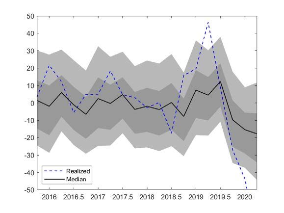
Figure 2 shows the fitted values of the conditional quantiles over time together with
the realised values for the aggregate sample of banks22 . While median/mean estimates
accurately represent the net trading income ratio during normal times, they perform poorly
during periods of financial distress. The realised value during the onset of the Covid-
19 pandemic markedly deviates from the median and average estimates. However, the
realised values lie within the conditional distribution. We also provide Figure A.12 in the
appendix which shows the conditional quantiles over time for two individual major banks
with significantly different variance.
20 These findings complement the existing quantile regression literature using non-linear quantile models.
Adrian, Boyarchenko, and Giannone (2019) and Chavleishvili and Manganelli (2019) show that an aggregated
financial condition index affects the left side of GDP growth distribution for US and EU respectively but
not the right tail.
21 We control for business model classification as defined by the ECB. Business model classifications cat-
egorise banks as G-SIBs, universal banks, investment banks, asset managers, custodian banks and various
types of lenders.
22 We aggregate the quantiles to form a combined distribution using a quantile averaging method known
as vincentization (see Ratcliff (1979) for further details). Vincentization is a simple method to combine
distributions by averaging α per cent quantiles to construct the α per cent quantile of the group where 0 <
α < 1. Therefore, if qi is the αP per cent quantile of Fi , that is Fi (qi ) = α then the predicted distribution
n
would be defined by F −1 (α) = w q . In our setting all the weights are the same.
i=1 i i
ECB Working Paper Series No 2525 / February 2021 18Figure 2: Fitted conditional quantile estimates from the quantile dynamic fixed effect panel
model.
Note: The panel shows the estimates over the period 2015-2020 at quarterly intervals for the
aggregate sample of banks. The aggregate sample distribution is combined using vincentization -
a quantile averaging method. The black line is the conditional median quantile, the shaded dark
grey defines the 30th to 70th quantiles and the lighter grey the 10th and 90th quantiles. The blue
dashed line shows the realised value.
As discussed in section 3, the method of moments approach has the advantage that it
is computationally easy to implement, and deals well with the incidental parameter and
quantile crossing problem. However, two sources of concern should be investigated. First,
the inclusion in the specification of the model of bank-specific variables among the regres-
sors can lead to endogeneity problems. Second, the presence of a auto-regressive regressive
23
component can lead to biased estimates.
As robustness check, we consider an alternative method to estimate the dynamic quantile
regression. In particular we use the iterative simulation-based approach framework devel-
oped by Arellano and Bonhomme (2016) to estimate the model. Under the assumption that
Ui,t given in equation 6 is independent from the vector (Xi,t ) where (Xi,t ) contains the two
23 The FE-OLS and FE-QAR estimators are biased in the presence of lagged dependent variables as
regressors, particularly for panels with a relatively short time series dimension; see for example,Galvao
Jr (2011) and (Nickell (1981)). Machado and Silva (2019) show in a simulation exercise that bias arising
from the method of moments should be small and not significantly affect the parameter estimates.
ECB Working Paper Series No 2525 / February 2021 19lagged values of Yt and under some starting values for the parameters we can consistently
recover the parameters numerically via an extension of the expectations maximization al-
gorithm.24 Following this procedure and setting as starting values the estimates of simple
quantile regression we estimate the parameters of equation 6 for quantiles 0.1 up to 0.9
shown in figure 3. The estimates and the paths of all variables with the exemption of eq-
uity over total assets are found to be in line with the estimates of the method of moments
approach shown in table 2. Overall, we can conclude that the results from the Arellano
and Bonhomme (2016) estimation confirm that our main findings are not an artifact of the
method of moments regression procedure but reflect a robust property of the conditional
distribution of net trading income.
Figure 3: Simulation based quantile Regression estimates for NTI/TA
Note: Parameter estimates from the dynamic quantile model with fixed effects estimated by Arel-
lano and Bonhomme (2016) simulation method. The sample period is 2015Q2 up to 2020Q1 and
the number of banks is 54.
As further robustness check, we estimate the model considering other macro-financial
controls. In particular, we replace equity returns by Itraxx senior financial returns, Vstoxx
with VIX and we added as additional regression 10 year sovereign spreads. Table 3 shows
that the significance and persistence of net trading income lagged variables hardly change
24 For more details on the estimation procedure see Arellano and Bonhomme (2016).
ECB Working Paper Series No 2525 / February 2021 20under this different specification. Swap spreads and credit spread parameters are somewhat
smaller while the FX parameters are bigger. Finally, consistent with financial indicators the
Itraxx senior financials is significant for higher quantiles. The sign is reverted compared to
table 2 as higher Itraxx returns reflect worsening financial conditions where for stock returns
is the opposite. Ad final robustness check, we include among the controls a business model
of banks and results remain substantially unchanged (see Table A.3).
5 Conditional net trading income distribution
The quantile equation (3) delivers an approximate empirical inverse cumulative distribu-
tion function (CDF)25 of the NTI/TA ratio for each quarter and each bank. Mapping the
estimates of the quantile function into a probability density function (PDF) is not straight-
forward because of estimation error and data noise. One way to address this problem is by
interpolating the quantile functions using splines and imposing monotonicity and smooth-
ness as in Schmidt and Zhu (2016). Alternatively, as shown by Adrian, Boyarchenko, and
Giannone (2019), we can recover the probability density function parametrically by fitting
parametric probability function.We therefore smooth the estimated quantile distribution
every quarter and for each bank by interpolating between the estimated quantiles using the
skewed t-distribution developed by Azzalini and Capitanio (2003). This methodology per-
mits the transformation of the empirical quantile distribution into an estimated conditional
distribution.
Following Azzalini and Capitanio (2003) we fit the following probability density function:
s !
2 y−µ y−µ ν+1
fY (µ, σ, α, ν) = t ;ν T α ;ν
y−µ 2
+1 (9)
σ σ σ ν+ σ
where t(·) and T (·) respectively denote the PDF and CDF of the Student t-distribution.
The four parameters of the distribution pin down the location µ , the scale σ, the fatness
25 The quantile function of a scalar random variable Y is the inverse of its cumulative distribution function.
ECB Working Paper Series No 2525 / February 2021 21Table 3: OLS and Quantile Regression estimates
NTI/TA × 10000 OLS Q1 Q3 Q5 Q7 Q9
NTI/TAt−1 × 10000 0.41∗∗∗ 0.41∗∗∗ 0.41∗∗∗ 0.41∗∗∗ 0.40∗∗∗ 0.40∗∗∗
(0.06) (0.09) (0.07) (0.06) (0.06) (0.08)
NTI/TAt−2 × 10000 -0.21∗∗∗ -0.17∗ -0.20∗∗∗ -0.21∗∗∗ -0.23∗∗∗ -0.25∗∗∗
(0.03) (0.09) (0.07) (0.06) (0.05) (0.07)
Equity on Total Assetst−1 55.51∗∗∗ 60.87 57.66 55.70 53.52 49.98
(20.47) (54.97) (42.83) (40.89) (45.66) (62.24)
REA on Total Assetst−1 3.38 -7.53 -1.00 2.98 7.41 14.61
(8.82) (9.84) (8.01) (8.26) (9.92) (13.95)
Swap Spread 10Y-3Mt 2.69∗ 2.40 2.58∗∗ 2.68∗∗ 2.80∗∗ 2.99∗
(1.55) (1.64) (1.26) (1.18) (1.27) (1.71)
Credit Spread (BBB - 10Y)t 1.55∗ 4.82∗∗∗ 2.86∗∗ 1.67 0.34 -1.82
(0.90) (1.71) (1.27) (1.17) (1.31) (1.85)
Oil returnst 1.52 7.26∗ 3.82 1.72 -0.61 -4.40
(2.03) (4.28) (3.15) (2.72) (2.77) (3.73)
∆ EUR-USDt -13.14∗ 24.24∗ 1.86 -11.79 -26.95∗∗ -51.63∗∗∗
(7.44) (13.33) (10.11) (9.66) (10.62) (15.08)
US VIXt -0.79 -7.94∗∗∗ -3.66∗∗ -1.05 1.85 6.58∗∗
(1.54) (2.53) (1.85) (1.69) (1.88) (2.62)
Sovereign yield 10Y - 10Y Swap t 1.48 -0.11 0.84 1.42 2.06 3.11
(1.22) (1.21) (1.09) (1.28) (1.67) (2.42)
Itraxx returnt -3.58∗ 5.93∗∗ 0.23 -3.24 -7.10∗∗∗ -13.38∗∗∗
(1.84) (2.67) (1.99) (1.98) (2.25) (3.14)
R2 0.177
Observations 1026 1026 1026 1026 1026 1026
Standard errors in parentheses
∗ p < 0.10, ∗∗ p < 0.05, ∗∗∗ p < 0.01
ECB Working Paper Series No 2525 / February 2021 22ν, and the shape α. Relative to the t-distribution, the skewed t-distribution adds the
shape parameter which regulates the skewing effect of the CDF on the PDF. Similarly to
Adrian, Boyarchenko, and Giannone (2019), we choose the four parameters µt , σt , αt , νt
every quarter in order to minimize the distance between our estimated quantile function
QYt (τ |Xt ) and the quantile function of the skewed t-distribution F −1 (τ |µt , σt , αt , νt ) to
match the 10th to 90th quantiles. Formally, for each bank i:
X 2
[µ̂t , σˆt , α̂t , νˆt ] = arg min QYt (τ |Xt ) − FY−1
t
(τ |µt , σt , αt , νt ) (10)
µ,σ,α,ν
τ
where µ̂t ∈ R, σ̂t ∈ R, α̂t ∈ R, ν̂t ∈ R+
Figure 4 shows the smoothed conditional distribution functions QYt (τ |Xt ) for two se-
lected periods: the last quarter of 2019 and the first quarter of 2020. The conditional
distribution is very sensitive to changes in financial risk factors. During the onset of the
Covid-19 pandemic the tails of the distribution have become fatter, especially the left tails
for many of the 54 selected banks. The visible shift to the left and fattening of the tails im-
plies that there is a higher probability of the bank experiencing both negative and extreme
NTI losses in following quarter.
6 Conditional expected shortfall and loss probability
In this section, we estimate expected losses given the sensitivity of a bank to system wide
risk factors. The smoothed conditional net trading income distribution is used to estimate
two tail risk measures - conditional expected shortfall and the material loss probability. As
shown in Adrian, Boyarchenko, and Giannone (2019) we can use the conditional distribution
to estimate expected shortfall (ES) and its upper tail equivalent expected longrise (EL). For
a given percentile α expected shortfall in the one-step ahead period can be defined as follows
Z α
1
ESt+1 = F̂y−1
t |Xt
(τ |Xt )dτ (11)
α 0
where F̂y−1
t |Xt
is computed according equation 10.
ECB Working Paper Series No 2525 / February 2021 23Figure 4: Conditional NTI/TA distribution.
(a) Conditional distribution Q4 2019
(b) Conditional distribution Q1 2020
Note: The panels show the estimated conditional smoothed distribution of equation (5) for NTI/TA.
The top panel shows the conditional distribution in Q4 2019, and the bottom panel in Q1 2020.
Each bank in the sample is represented along the z-axis. NTI/TA is presented in basis points.
ECB Working Paper Series No 2525 / February 2021 24In the upper tail longrise is defined as
Z 1
1
LRt+1 = F̂y−1
t |Xt
(τ |Xt )dτ (12)
α 1−α
The 5% expected shortfall is the conditional expectation of NTI loss, conditional on an
NTI loss being below the 5th percentile of the conditional distribution. For the purpose of
assessing expected shortfalls and loss probabilities we measure NTI relative to RWAs26 to
allow for comparison to CET1 ratios.27 We define an NTI loss greater than 15bps of total
RWAs as material. Since expected shortfall (longrise) is an average over all losses in the tail
that exceed a value at risk defined at α percentile of the conditional distribution it is very
sensitive to NTI losses (profits) deep in the tail. This makes an appealing tail risk measure
as it can capture fat tails which are characteristically present in financial distributions such
as NTI.
To estimate the material loss probability (MLP) we ask what is the probability that a
loss is material in the next quarter (exceeds 15bps of total RWAs):
Z 0.0015
M LPt+1 = F̂yt |Xt (τ |Xt )dτ (13)
0
where F̂yt |Xt is the CDF of the fitted skewed t-distribution estimated according to equa-
tion 10.
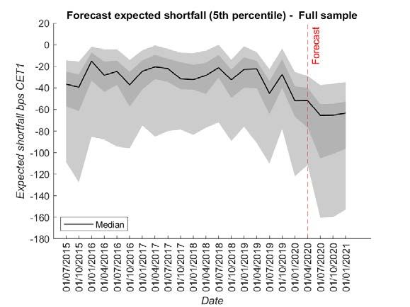
Figure 5 shows the conditional expected shortfall at 5 and 10 percent levels for the full
sample of banks. The conditional distribution changes over time and is extremely sensitive
to shocks in financial risk factors. Based on the estimated model the Covid-19 crisis leads
to a marked increase in expected CET1 loss at both 5 and 10 percent in the first quarter
of 2020. In the 5 percent tail there is wide variation across banks as shown in Figure 5
expected losses vary from 20bps to 120bps for banks at the extremes, evidence of fat tails
shown in the conditional NTI distribution. At the height of the Covid-19 crisis all 54 banks
26 In order to derive this ratio, we multiplied NTI by TA and divided it by RWA.
27 The standard regulatory benchmark for measuring bank solvency is the common equity tier 1 (CET1)
ratio, measured as common equity capital relative to risk weighted assets (RWAs). Under European capital
requirement regulation (CRR) banks are required to hold a minimum amount of regulatory capital to ensure
they can withstand stress. CET1 capital is the highest quality capital that a bank holds and will be the
first to absorb losses.
ECB Working Paper Series No 2525 / February 2021 25have a 5% expected capital shortfall greater than a material loss of 15bps RWAs, and 43
banks have a 10% expected shortfall greater than 15bps RWAs. This means that if a bank
experiences a tail loss the expectation is that it will be material.
Figure 5: Conditional expected capital shortfall.
Note: The graph shows expected shortfall for banks over the sample period 2015 - 2020 Q1 as
defined in equation (11). The upper panel shows the 5% expected shortfall and the lower panel
shows the 10%. Each quarterly observation on the graph shows the cross sectional distribution
across the sample of banks. The black line represents the bank with the median expected shortfall,
the shaded dark grey defines the banks at the 30th to 70th quantiles and the lighter grey the 10th
and 90th quantiles. Expected shortfall is expressed in basis points of NTI/RWA.
ECB Working Paper Series No 2525 / February 2021 26For most banks in the sample the extreme left tail quantile is more sensitive to risk
factor shocks than less extreme quantiles. Figure 6 shows the upper tail of the conditional
distribution and measures the expected growth in NTI conditional that the growth is above
the 95th percentile. The upper tail of the conditional NTI distribution is also highly sensitive
to changes in financial conditions. We find that both right and left tails of the conditional
NTI distribution to be sensitive to changes in financial conditions.28
Figure 6: Conditional expected capital longrise.
Note:The graph shows the conditional expected capital growth conditional on NTI/RWA being
above the 95th percentile as defined in equation (12). Each quarterly observation on the graph
shows the cross sectional distribution across the sample of banks. The black line represents the
bank with the median expected longrise, the shaded dark grey defines the banks at the 30th to
70th quantiles and the lighter grey the 10th and 90th quantiles. Expected longrise is expressed in
basis points of NTI/RWA.
Figure 7 shows the probability of a material NTI loss occurring in the following quarter.
The chart illustrates the increase in probability in the first quarter of 2020 with the median
probability of experiencing a an NTI loss greater than 15bps total RWAs in Q2 2020 is 37
percent.
28 Unlike Adrian, Boyarchenko, and Giannone (2019) who find that the left tail of the GDP growth to be
sensitive to financial conditions and the right tail stable over time.
ECB Working Paper Series No 2525 / February 2021 27Figure 7: material loss probability.
Note: The graph shows the short term probability of a loss being equal to or exceeding 15bps in
the following quarter as defined in equation (13).Each quarterly observation on the graph shows
the cross sectional distribution across the sample of banks. The black line represents the bank with
the median probability of exceeding 15bps, the shaded dark grey defines the banks at the 30th to
70th quantiles and the lighter grey the 10th and 90th quantiles.
7 Forecasting stress net trading income and the ex-
pected shortfall
We can use the model to generate forecasts n-periods ahead conditional on different stress
scenarios. Given the non-recursive specification of our setting we must specify the dynamics
of the exogenous parameters. We adopt a simple approach and we assume that each ex-
ogenous variable follows a quantile autoregressive process29 . Then, we iterate forward the
Q-AR(1) process to derive density forecasts for each variable. In a second step we lag the
forecast and we iterate forward to generate n-steps ahead density forecasts for the NTI30 . We
adopt two different approaches in order to project reasonable NTI values. First, we assume
29 Variables with a panel dimension follow a panel quantile process (i.e. as for country-level equity indices)
30 A potential problem with this approach is that the predicted density often exhibits, in finite samples,
“quantile crossing” — that is, the predicted conditional quantile function is not monotonically increasing
in q. A potential solution is developed by Chernozhukov, Fernández-Val, and Galichon (2010) that suggest
the rearrangement of the predicted quantile function to make it monotone. This alternative was ensuring
monotonicity, but the forecast NTI was experiencing extreme behaviour in the tails of the distribution when
coupling tail estimates with tail realization of the explanatory variables.
ECB Working Paper Series No 2525 / February 2021 28that a static-balance sheet assumption holds as it is customary in the EU-wide Stress Test
Exercise. That is, bank-level explanatory variables stay constant over the forecast horizon.
Second, we project the quantile realizations of NTI using the the median realization of the
risk factors.
Risk-factors follow therefore this process:
QX (τ |Xt−1 ) = v(q) + m(q)Xt−1 + ut (14)
While bank-level variables evolve, for each quantile, as follow:
Xt+1 = Xt (15)
For n-step ahead forecasts we iterate equations (14) and (15) recursively for each quantile
and we plug the median density forecast into the fitted equation (7).
Table 4 shows descriptive statistics for the conditional forecast quantiles. We report
statistics for NTI/TA for 4 stress scenarios and the baseline scenario one year ahead (Q4
2020). We define the baseline scenario as the median NTI forecast for each bank. The
four adverse scenarios are defined as the conditional forecast at 10th, 20th, 30th and 40th
percentiles of the NTI over total assets in order to capture higher degree of severity.
We can visualise the conditional NTI forecasts in Q4 2020 using a kernel density esti-
mation in figure 8a. The wide dispersion of losses and long left tail is especially clear in
the most severe scenarios. We see a similar picture when we aggregate losses over each of
the quarters of 2020 as shown in figure 8b. The joint distribution of the conditional NTI
forecast in the baseline and adverse 4 scenario is shown in figure 9.
ECB Working Paper Series No 2525 / February 2021 29You can also read