2019 U.S. Housing Market Outlook - February 2019 - Pretium Partners
←
→
Page content transcription
If your browser does not render page correctly, please read the page content below
2019 U.S. Housing Market Outlook

                                   February 2019
Pretium’s 2019 Housing Market Outlook
We expect structural imbalances in the U.S. housing market will continue, leading to further tightening of
fundamentals and higher shelter costs
The most important issue in the housing market remains a persistent underbuilding of housing combined with accelerating
demand for shelter.
In 2018, housing demand exceeded supply by more than 400,000 units. 1 We forecast that the U.S. will continue to
underproduce housing by ~200,000 units in both 2019 and 2020, and vacancy rates should fall ~15bps each year.
Housing availability is tight, with the vacancy rate of for-sale and for-rent housing at 3.2%, the lowest level since 1984. 2
Constrained availability and further increases to replacement costs (labor, materials, land, and soft costs) should place
upward pressure on rental rates and home prices.
Higher mortgage rates negatively impacted homebuyer affordability, which we expect will drive incremental demand for
rental housing going forward.
Demand to remain elevated on the heels of a healthy economy and supported by demographic tailwinds, while the
growth in new supply begins to stall
During the first three quarters of 2018, the U.S. added 1.48mn households relative to the same period in 2017, the fastest
pace since 2015. 3
We expect above-average housing demand over the medium-term. The positive outlook for household formations is
supported by a strong labor market and historic demographic shifts, including the ageing of the Millennial generation, which
should sustain ~1.2-1.3mn household formations per annum going forward. 4
Single-family and multifamily housing starts added ~1.0mn new housing units in 2018 net of units lost to obsolescence.
Starts are plateauing, with consensus forecasting starts to increase by 10,000 in 2019 and another 20,000 in 2020. 5
Weaker homebuyer affordability will impact for-sale housing but should support incremental renter demand
Mortgage rates averaged 4.54% in 2018, 55bps higher than in 2017. 6 Higher rates were a headwind to transaction activity.
The median-income buyer of a median-priced home spent 37% of their income on mortgage, principal, insurance, and tax
payments in 4Q’18, in-line with an average of 38% since 1985, but well above the 32% average over the last five years. 7
We expect that a decline in homebuyer affordability, coupled with strong household formations, should support demand for
rental assets including single-family rentals and multifamily apartments.
Within U.S. real estate, we believe the single-family rental (“SFR”) sector is well positioned to capitalize on the
underbuilding of shelter and decline in affordability, capturing demand and driving further margin expansion
We believe residential real estate is well positioned to capture the secular increase in housing demand with less risk from
technological disruption or shift in consumer preference.
Young families should continue to seek the amenities of single-family housing, with more choosing to rent given affordability
headwinds and constraints on mortgage credit availability.
Institutionally-managed SFR has the potential to drive above-average net operating income (“NOI”) growth over the next
several years, coupling growing demand with revenue-generating and cost-saving technologies that should result in
continued margin expansion.
1 U.S. Census Bureau, Housing Vacancies and Homeownership Report, Table 3, as of 3Q’18.
2 U.S. Census Bureau, Housing Vacancies and Homeownership Report, Table 2, as of 3Q’18.
3 U.S. Census Bureau, Current Population Survey/Housing Vacancy Survey, Table 13a. Monthly Household Estimates, October 30, 2018.
4 Morgan Stanley, “U.S. Housing Tracker – January”, January 4, 2019. Harvard JCHS, “Updated Household Growth Projections: 2018-2028”, December 2018.
5 Bloomberg Weighted Average Consensus Forecast, January Survey, 2019 and 2020 Housing Starts, retrieved January 11, 2019.
6 Freddie Mac, 30-Year Fixed Rate Mortgage, retrieved from FRED, Federal Reserve Bank of St. Louis, January 10, 2019.
7 Pretium calculation using Moody’s income data, U.S. Census and NAR existing home price data, Fannie Mae 30Yr Mortgage rates, FHA mortgage insurance premiums,
as of December 27, 2018.
2019 U.S. Housing Market Outlook 1
Section I: 2019 Economic Outlook
Healthy Economic Growth in 2018 Expected to Continue Through 2019
The U.S. economy is performing well, supported by healthy job growth, corporate tax reform, and elevated consumer and business
confidence. We continue to see the U.S. economy as mid- to late-cycle, but not late-cycle given the healthy and, in many cases,
accelerating growth in key metrics:
Real GDP grew 3.0% in the third quarter on a year-over-year basis (and 4.1% Q/Q annualized), an acceleration from 2.4%
Y/Y growth in 2017 and 1.9% in 2016. 8 Consensus estimates from Wall Street economists forecast real GDP growth of 2.5%
for 2019, and 1.8% for 2020. 9
Non-farm employment grew 1.8% Y/Y in December, with the U.S. creating an average of 220k jobs per month during 2018,
an acceleration from the 180k pace in 2017. 10
Unemployment fell from 4.1% at the end of 2017 to 3.9% in December 2018. Wall Street economists forecast unemployment
to compress further to 3.6% by year-end 2019. 11
Tightening labor markets led to improving wage growth and increased labor participation. Average hourly earnings
increased 3.3% Y/Y in December, 12 while the Employment Cost Index rose 2.8% Y/Y in 3Q’18, the fastest pace since 2008. 13
Consumer confidence reached its highest post-crisis levels in 2018, with the University of Michigan Consumer Sentiment
Index reaching its highest levels since 2001 in early 2018. 14
Business activity was positive. Purchasing Managers’ Indices (“PMIs”) for services and manufacturing averaged 55 (index
level above 50 indicates improving conditions) for full year 2018 and confidence measures such as the NFIB Small Business
Optimism Index were at above-average levels. Capex spending grew 8% Y/Y. 15
Exhibit 1: Healthy Labor Markets Supporting Cycle High Wage Growth
4,000 4% 11%
10%
2,000 2% 9%
8%
0 0% 7%
6%
-2,000 -2%
5%
-4,000 -4% 4%
3%
-6,000 -6% 2%
1%
-8,000 -8% 0%
1995
1997
1999
2001
2003
2005
2007
2009
2011
2013
2015
2017
1995
1997
1999
2001
2003
2005
2007
2009
2011
2013
2015
2017
2019
Total Non-Farm Payrolls, Y/Y % (rhs)
Unemployment Rate Avg. Hourly Earnings Growth
Total Non-Farm Payrolls, Y/Y Change (000's, lhs)
Source: U.S. Bureau of Labor Statistics, All Employees: Total Nonfarm Payrolls, Civilian Unemployment Rate, Average Hourly Earnings of
Production and Nonsupervisory Employees: Total Private, through December 2018.
8 Bureau of Economic Analysis, Gross Domestic Product, 3Q’18.
9 Bloomberg Weighted Average Consensus Forecast, January Survey, 2019 and 2020 Real GDP Growth forecast, retrieved January 11, 2019.
10 U.S. Bureau of Labor Statistics, All Employees: Total Nonfarm Payrolls, through December 2018.
11 U.S. Bureau of Labor Statistics, Civilian Unemployment Rate, through November 2018. Wall Street forecasts are Bloomberg consensus, retrieved January 10, 2019.
12 U.S. Bureau of Labor Statistics, Average Hourly Earnings of Production and Nonsupervisory Employees: Total Private, through December 2018.
13 U.S. Bureau of Labor Statistics, Employment Cost Index: Total compensation: All Civilian, through 3Q’18.
14 University of Michigan, University of Michigan: Consumer Sentiment, data through November 2018.
15 Markit Service PMI and Manufacturing PMI, data through December 2018, retrieved from Bloomberg on January 4, 2019. NFIB Research Foundation, Small
Business Optimism Index, through December 2018. Bureau of Economic Analysis, 3Q’18 data on gross private domestic investment.
2019 U.S. Housing Market Outlook 2
Employment an Important Driver of Housing Demand
A healthy economic backdrop is important to our constructive outlook for housing demand and pricing power. Employment growth
is a key driver (along with population growth, consumer confidence, and housing availability) of household formations, as illustrated
by Exhibit 2 below. Further, housing is pro-cyclical, and economic growth (e.g., GDP, employment, wages, labor force participation)
has historically translated into improving asset values. 16
Exhibit 2: Household Formations and Employment Growth are Closely Linked

                                       2,500                                                                                             4,000

                                                                                                                                                   Y/Y Full Time Payrolls (000s)
                                       2,000                                                                                             2,000
     HH Formations (000s)

                                       1,500                                                                                             -

                                       1,000                                                                                             (2,000)

                                           500                                                                                           (4,000)

                                             0                                                                                           (6,000)

                                              Household Formations (LHS, Tr. 2Yr)          Full-Time Employment Growth (RHS, Tr. 2Yr)

Source: U.S. Census Bureau, Current Population Survey/Housing Vacancy Survey, Table 13a. Monthly Household Estimates, October 30, 2018. U.S.
Bureau of Labor Statistics, All Employees: Total Nonfarm Payrolls, December 2018.

While household formations have rebounded, we estimate pent-up demand includes nearly 5mn “missing”
households, particularly among younger cohorts as more young adults are living at home. As shown below on the left,
there has been a sharp increase in young adults living at home; from 2003 to 2017, the percentage of 18- to 34-year-olds living at
home increased from 27% to 31%, an increase of over 3mn people. 17 Deferred household formations are reflected in lower headship
rates / deferred household formation relative to expected housing demand.
Better employment and wage growth for these cohorts may encourage a decline in young people living at home and, therefore,
additional household formations. Employment of 25- to 34-year-olds increased by more than 5.8mn since 2010, or ~31% of all net
employment growth. Year-over-year 25- to 34-year-old employment rose 3.1%, 100bps faster than general employment growth. 18
Note, projections from Harvard’s Joint Center for Housing Studies (“JCHS”) for 1.22mn household formations per annum through
2028 assume no change to headship rates. Therefore, a return of these missing households would be additive to their estimates. 19
Exhibit 3: Pent-Up Demand Led by Under 35 Cohorts Who Increasingly Live at Home

                                           4,500                                                                                        Cumulative "Missing" Households due to Lower
                                                                                                                                                       Headship Rates
              18- to 34-year-olds (000s)

                                                       Post-Crisis                                                             1,000
                                           3,500       Increase in
                                                                                                           Households (000s)

                                                       Young People
                                           2,500
                                                       Living at Home                                                          -1,000
                                           1,500                                                                                             Post-Crisis
                                                                                                                                             Deferred
                                            500                                                                                -3,000        Household
                                                                                                                                             Formation
                                           -500
                                                                                                                               -5,000

                                              Cumulative increase in 18- to 34-year-olds at home                                 Under 35    35 to 44                              45 to 54   55 to 64   65 and over

Source: U.S. Census Bureau, Current Population Survey/Housing Vacancy Survey, July 26, 2018 and U.S. Census Bureau, National Intercensal Tables
2000-2010, and National Population by Characteristics: 2010-2017. Table AD-1. Young Adults, 18-34 Years Old, Living At Home: 1960 to Present.

16 U.S. Census Bureau, Current Population Survey/Housing Vacancy Survey, Table 13a. Monthly Household Estimates, October 30, 2018.
17 U.S. Census Bureau, Table AD-1. Young Adults, 18-34 Years Old, Living At Home: 1960 to Present, November 16, 2017.
18 U.S. Bureau of Labor Statistics, Employment Level: 25 to 34 years, Civilian Employment Level, as of December 2018.

19 Harvard JCHS, “Updated Household Growth Projections: 2018-2028”, December 2018.

2019 U.S. Housing Market Outlook                                                                                                                                                                                       3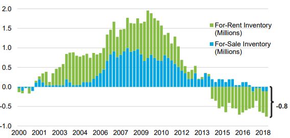
Bond Yields: 2018 Increase Moderated in 4Q, but Risks to Upside in 2019
The risk-free rate curve increased and flattened in 2018, as the market responded to tighter monetary policy, but
also priced in more concern about sharply lower growth in the medium-term.
On the short end, the Federal Reserve raised overnight rates four times in 2018 to 2.25%-2.50%, with their latest forecast
expecting two additional rate increases in 2019. That said, in January 2019, Federal Reserve Chairman Powell attempted
to calm market concerns of the Fed moving too fast with policy normalization, noting monetary policy is not a “pre-set”
course, with the Fed monitoring economic data and financial conditions closely.
On the longer-end, 10Yr Treasuries increased by 30bps to 2.7% at year-end, but were as high as 3.3% in October before
retreating on global growth concerns. The yield curve, therefore, flattened significantly with the spread between the 2Yr
Treasury and 10Yr Treasury just 20bps at year-end from 52bps at the end of 2017. 20
Our outlook for rates in 2019 is for higher rates across the curve.
On the short end, while the Federal Reserve has made it clear it intends to be patient with the pace of further rate hikes, we
believe they will raise rates one or two times in 2H 2019 due to the strength of the labor market and inflationary pressures
from tariff policy.
On the long-end, we believe the combination of the Fed balance sheet runoff (i.e. quantitative tightening or “QT”), additional
Treasury supply to satisfy the increasing funding needs of the U.S. government and net issuance from U.S. corporates will
pressure yields and spreads for long-dated fixed income.
Exhibit 4: Net Annual Change in Combined Federal Reserve, European Central Bank, and Bank of Japan Balance Sheets
$2,500
$2,000
$1,500
Global central banks are
$1,000 expected to withdraw liquidity
$500 from the financial system on a
year-over-year basis for the first
$0 time since 2009
-$500
Source: Bloomberg, priced on January 10, 2019.
Exhibit 5: U.S. Treasury Expected to Issue More Than $1tn of Debt in 2019-2022 to Fund Growing Deficit
$0
($200)
($400)
The U.S. Treasury is expected to
($600)
issue $1.00tn of debt to fund its
($800) 2019 budget deficit, up from
($1,000) ($779)
$665bn in 2017
($1,200) ($1,000)
($1,125)
($1,400)
($1,600)
Source: Goldman Sachs estimates, from the ERWIN forecast database, accessed on January 10, 2019.
20 Bloomberg, priced on January 25, 2019.
2019 U.S. Housing Market Outlook 4Mortgage Rates Increased ~55bps Y/Y, Impacting Affordability and Home Sales
Since the beginning of 2018, 30-year fixed mortgage rates rose sharply, ending the year at 4.55% with the rate averaging ~55bps
higher during the year than in 2017. This increase came after a 30bp increase in mortgage rates in both 2016 and 2017. Rising rates,
coupled with a level of HPA above nominal income growth, are significantly impacting affordability. 21
However, as shown in Exhibit 6 below, mortgage rates have recently eased as markets have altered their views on the outlook for
economic growth and future Federal Reserve rate hikes. A gentler increase in rates, as opposed to the late-2018 spike, could benefit
the housing market in 2019.
Exhibit 6: 30-Year Mortgage Rates Up from Historic Lows
5.5%
Avg. 30-Year Fixed
5.0% Mortgage Rate
4.55% 2015 3.9%
4.5%
2016 3.7%
4.0%
2017 4.0%
3.5%
2018 4.5%
3.0% 4Q’18 4.8%
Jul-10
Jul-11
Jul-12
Jul-13
Jul-14
Jul-15
Jul-16
Jul-17
Jul-18
Jan-10
Jan-11
Jan-12
Jan-13
Jan-14
Jan-15
Jan-16
Jan-17
Jan-18
Source: Freddie Mac, 30-Year Fixed Rate Mortgage Average, retrieved from FRED, Federal Reserve Bank of St. Louis; December 27, 2018.
Higher rates negatively impacted homebuyer affordability, which is now back to pre-crisis levels after having been
much more affordable post-crisis due to low mortgage rates and depressed home values. One way to show affordability
is to estimate median home payment-to-income ratios over time. In 4Q’18 this index showed that the median U.S. family buying a
median-priced home would spend 37% of its income on home payments, in line with the 38% average since 1985 and well above the
32% average over the past five years. 22
Housing payments have increased rapidly on the back of higher rates and rising home prices. The implied monthly mortgage and
insurance payment in 4Q’18 was 13% higher than in 4Q’17, and 19% higher than in 4Q’16. 23
Exhibit 7: Affordability at Long-Term Average with Median New Purchase Home Payments Up ~13% Y/Y
Components of Y/Y Change in Payment
55% 15%
Home Payment as % of Income
50%
10%
45%
40% 5%
35% 0%
30%
-5%
25%
20% -10%
LT Avg (since 1985) Payment as a % of Income Δ Rates Δ Home Prices Δ Taxes, Insurance, PMI, etc
Source: Pretium calculation using Moody’s income data, U.S. Census and NAR existing home price data, Fannie Mae 30Yr Mortgage rates, FHA
mortgage insurance premiums, as of December 27, 2018.
21 Freddie Mac, 30-Year Fixed Rate Mortgage, retrieved from FRED, Federal Reserve Bank of St. Louis; December 27, 2018.
22 Pretium calculation using Moody’s income data, U.S. Census and NAR existing home price data, Fannie Mae 30Yr Mortgage rates, FHA mortgage insurance
premiums, and the forward treasury curve from Bloomberg as of January 10, 2019. For all periods, calculation assumes a 96.5% LTV FHA loan with 85bps of
mortgage insurance, taxes equal to 1.2% of home value, insurance equal to 50bps of home value, and HOA fees of 15bps of home value.
23 Freddie Mac 30-Year Fixed Rate Mortgage Average. Data sourced from St. Louis Fed FRED system on December 27, 2018.
2019 U.S. Housing Market Outlook 5Affordability Headwinds Positive for Rental Outlook
We believe that weaker new homebuyer affordability at a time of strong household formations will increase rental
demand as households, on the margin, find home buying less affordable and have less inventory from which to
choose. We expect single-family rental demand will increase and length of stay should increase.
SFR is one-third of the rental market and should therefore benefit as more households rent. Further, single-family detached
homes share many of the amenities of for-sale, entry-level housing which are attractive to residents, especially those with
children (access to schools, more square footage inside and outside of the home).
It is important to emphasize that SFR has historically represented a large share of rentals and overall housing. Since 1970,
single-family rentals have comprised, on average, ~11.5% of U.S. housing and ~33% of rental housing. 24
In a recent report, John Burns Real Estate Consulting emphasized the positive SFR demand impact of worsening
affordability, “Worsening affordability should keep SFR tenants in place longer, as an increasing amount will not be able to
qualify for a mortgage as rates and home values rise.” 25
We do not expect higher rates to materially impact positive trends in household formations. Economic growth,
coupled with the ageing of the Millennial generation, is likely to produce significant housing demand as these younger cohorts age
into their early- to late-30s over the next decade.
Interestingly, to date, younger cohorts have not driven the positive trends in household formation. According to Morgan
Stanley, “25- to 29-year-olds have not formed households this slowly in 55 years. For 30- to 34-year-olds, headship rates
are at 46-year lows.” 26
In our view, the homeownership rate is unlikely to move higher in the coming years, which should add to
incremental rental demand.
We expect that constrained mortgage credit availability and weak affordability will lead more households to rent, even before
considering any potential change in homebuyer preference due to generational attitudes, weaker young adult balance sheets,
etc.
Interestingly, a recent Urban Institute report points to evidence of a shift in housing preference among Millennials not
explained by changing family dynamics or credit conditions. For example, homeownership for 25- to 34-year-old married
couples with children was 56.6% in 2015, down ~900bps from 2005 and 540bps from 1990 levels. 27
Exhibit 8: Single-Family Rentals as a Percent of U.S. Housing (left) and Rentals (right)
15% 40%
12.4%
34.5%
36%
10%
32%
28%
5%
24%
0% 20%
SFR as % of Housing LT avg SFR as % of Rentals LT avg
Source: U.S. Census Bureau. For 1970-1995 data, we use the American Housing Survey data. For 2000 and 2010 we use the Decennial Census. For
2005, 2015, and 2017 we use the American Community Survey 1 Year Survey. Any error in combining these various data series is ours.
24 U.S. Census Bureau. For 1970-1995 data, we use the American Housing Survey data. For 2000 and 2010, we use the Decennial Census. For 2005, 2015, and 2017,
we use the American Community Survey 1-Year Survey.
25 John Burns Real Estate Consulting, “Single-Family Rental Analysis and Forecast”, November 2018.
26 Morgan Stanley, “2019 U.S. Housing and Resi Credit Outlook: Slow and Steady,” November 30, 2018.
27 Urban Institute, “Millennial Homeownership, Why Is It So Low, and How Can We Increase It?” July 2018.
2019 U.S. Housing Market Outlook 6Limited Inventory and Affordability Concerns Slowing Pace of Home Sales
Rising rates and deteriorating affordability are slowing activity in a housing market that is coming off of
record low for-sale inventory levels.
In December, the monthly volume of existing home sales fell 10.3% from last year, the biggest Y/Y decline since 2011. However, for
the year, the average rate of existing homes sales fell a more modest 3.5% compared to the average rate in 2017. 28
Deterioration in affordability due to higher mortgage rates has slowed existing home sales further, but so have low inventory levels,
which averaged 4.2 months’ supply in 2H’18. Inventory levels reached a low of 1.3mn in December 2017 with only 3.1 months of
supply.
Morgan Stanley’s housing research team noted that “decreased affordability is weighing on transaction volumes…While we believe
affordability to be the chief culprit, the lack of supply is not helping matters… We expect these pressures to remain in 2019.” 29 While
sales were down Y/Y, the pace is generally in-line with long-term historical averages at 4.4% of U.S. housing stock. 30
Exhibit 9: Existing Home Sales, Absolute (left) and as Percent of Housing Stock (right)
7,500 50% 7.0%
7,000 40% 6.5%
6,500 30% 6.0%
6,000 20% 5.5%
5,500 10%
5.0%
5,000 0%
4.5%
4,500 -10%
4.0%
4,000 -20%
3.5%
3,500 -30%
3,000 -40% 3.0%
Existing Home Sales as % of Total Housing Units
Existing Home Sales (SAAR) Δ YoY
Avg Sales as % of Housing Units, 1985-2018
Source: National Association of Realtors, Existing Home Sales, through December 2018. U.S. Census Bureau, Current Population Survey/Housing
Vacancy Survey, October 30, 2018.
28 National Association of Realtors, Existing Home Sales, December 2018.
29 Morgan Stanley, “2019 U.S. Housing and Resi Credit Outlook: Slow and Steady,” November 30, 2018.
30 U.S. Census Bureau and National Association of Realtors, Existing Homes Sales report, through December 2018.
2019 U.S. Housing Market Outlook 7Rising rates are also putting new home sales and pricing under pressure as the price gap between new and existing
homes narrows.
During this housing cycle, median new home sales prices accelerated more quickly than existing home sales prices. By 2014, the
median sales price of a new home was 34% higher than the median existing home compared to an average new home premium of
18% from 1980 to 2006. 31
Due to growing inventory and builder emphasis on smaller homes, the median sales price of new homes stayed flat in 2018. On the
other hand, the median sales price of existing homes increased ~5% Y/Y due to tight inventory levels.
As shown on the right below, this dynamic has narrowed the gap between new and existing median sales prices to 24%, the smallest
since 2009. 32 We expect the gap to narrow further given the scarcity of existing homes for sale and deteriorating trends in the new
home market.
Exhibit 10: New Homes Sales Below 550k Annual Pace Exhibit 11: New and Existing Sales Price Gap Narrowing
800 14 $350k
700
12 $300k
New Home Sales (000s)
600
Median Sales Price
Months Supply
10 $250k
500
400 8 $200k
300
6 $150k
200
4 $100k
100
0 2 $50k
New Home Sales (SAAR) Months Supply Existing Homes New Homes
Source: U.S. Census Bureau and the National Association of Realtors, data through November 2018. U.S. Census Bureau, Median Sales Price of
Houses, as of November 2018; U.S. Census Bureau and U.S. Department of Housing and Development, Median Sales Price for New Houses Sold, as
of October 2018.
31 U.S. Census Bureau, Median Sales Price of Houses, as of November 2018; U.S. Census Bureau and U.S. Department of Housing and Development, Median Sales Price
for New Houses Sold, as of October 2018.
32 Ibid.
2019 U.S. Housing Market Outlook 8Home Price Appreciation Decelerated in 2018, but Remains Elevated
Housing values continued to rise at an above-inflation pace in 2018 due to steady demand growth, rising input costs, and below
average inventory levels. CoreLogic estimates that home prices grew 5.1% Y/Y through November 2018, down from a peak rate of
6.6% in March.
HPA growth decelerated from a recent peak in early 2018 as deteriorating affordability provided a headwind to buyers. Although the
slowdown has been nationwide, higher-price point markets and those with the fastest HPA have been most adversely impacted. The
most significant deceleration in HPA occurred in previously fast-growing markets facing affordability issues including Seattle and
several California markets. 33
Exhibit 12: Home Price Appreciation Has Decelerated Nationally
7.5%
7.0%
6.5%
6.0%
5.5%
5.0%
4.5%
Pretium Markets YoY HPI National YoY HPI
Source: CoreLogic Home Price Index, Single-Family Combined Tier, as of November 2018. “Pretium Markets” include Atlanta, Charlotte, Dallas,
Houston, Indianapolis, Jacksonville, Las Vegas, Memphis, Miami, Nashville, Orlando, Phoenix, Raleigh-Durham, and Tampa-St. Petersburg.
Post-crisis, lower-priced homes have outperformed higher-priced homes. According to CoreLogic, since 2010 the
highest-priced tier of homes has appreciated a cumulative 40%, while the lowest-priced tier of homes has appreciated over 76%.
Although HPA slowed down for all price tiers in 2018, low-priced homes are still outperforming high-priced homes by over 3%, down
from over 4% in early 2017. 34
Exhibit 13: Lower Price Points Still Outperforming due to Tighter Inventory Levels
10.0%
9.0%
Y/Y HPA by Price Tier
8.0%
7.3%
7.0%
6.0% 6.0%
5.4%
5.0%
4.0% 4.2%
3.0%
High price Middle-to-moderate price
Low-to-middle price Low price
Source: CoreLogic Home Price Index, Single-Family Combined Tier, as of November 2018.
33 CoreLogic Home Price Index, Single-Family Combined Tier, as of November 2018.
34 CoreLogic Home Price Index, Single-Family Combined Tier, as of November 2018. The four price tiers are based on the median sale price and are as follows: homes
priced at 75 percent or less of the median (low price), homes priced between 75 and 100 percent of the median (low-to-middle price), homes priced between 100 and
125 percent of the median (middle-to-moderate price) and homes priced greater than 125 percent of the median (high price).
2019 U.S. Housing Market Outlook 9U.S. Home Prices ~6% Above Prior Peak on a Nominal Basis
U.S. home prices have appreciated since 2012 and are now ~5.8% above the prior peak on a nominal basis. Adjusted for
inflation, home prices are 14% below the prior peak. 35 Further, it is important to recognize the pace and reasons why home
prices appreciated this cycle compared to the last cycle.
In the last housing cycle, U.S. home prices increased by 9.4% in 2002, 10.8% in 2003, 15.7% in 2004, and 15.3% in 2005
before flattening in 2006 and starting their decline in 2007. 36 This pace of appreciation was well above household income
growth and, arguably, fueled by loose credit and speculation more than fundamentals.
In this cycle, price gains have been more measured, with national HPA of 5.0% in 2014, 5.7% in 2015, 5.6% in 2016, and
6.2% in 2017. 37 This pace is more consistent with both strong fundamental demand and income growth, and the rising
costs of new home construction due to land, labor, materials, and regulatory costs.
According to Zelman & Associates, homebuilder labor and materials inflation has accelerated from +3.8% Y/Y in 2017,
to +4.9% Y/Y from November 2017 to November 2018. To offset cost inflation, new home prices appreciated 7.3% in 2017
and 8.6% from January 2018 through November 2018. 38
Evercore-ISI’s homebuilding research summarized this dynamic as, “Unlike the rampant speculative buying that marked the last
housing bubble, today’s demand is far more need-based, driven by significant pent-up demand for household formations that is
now being released.” 39
Exhibit 14: CoreLogic Nominal Home Price Index
300
250
Nominal home prices are 6%
200 above their prior peak level
150
100
50
US Home Price Index (Nominal) Prior Peak
Source: CoreLogic National HPI, updated through November 2018.
Exhibit 15: CoreLogic Home Price Index, Adjusted for Inflation
200
Adjusted for inflation, home
150 prices are 16% below their
prior peak level
100
50
US Home Price Index (Real) Prior Peak
Source: CoreLogic National HPI, updated through November 2018. Index deflated using U.S. Bureau of Economic Analysis, Personal Consumption
Expenditures Excluding Food and Energy (Chain-Type Price Index), downloaded from the St. Louis FRED data system on January 9, 2018.
35CoreLogic National HPI, updated through November 2018. Index deflated using U.S. Bureau of Economic Analysis, Personal Consumption Expenditures Excluding
Food and Energy (Chain-Type Price Index), downloaded from the St. Louis FRED data system on January 9, 2018.
36 CoreLogic National HPI, through November 2018.
37 CoreLogic National HPI, through November 2018.
38 Zelman and Associates, “Homebuilding Survey: Hoping for a Spring Turnaround”, December 12, 2018.
39 Evercore-ISI, “The Sun Also Rises: Upgrading the Homebuilders”, October 25, 2018.
2019 U.S. Housing Market Outlook 10Rates and Their Impact on HPA
Earlier we discussed the rise in mortgage rates during 2018 and the prospect for higher rates. Historically, home prices have exhibited
little correlation with mortgage rates. Other parts of the housing market, including starts and new/existing home sales, exhibit higher
negative correlations to rates than home prices.
In March 2018, we reported on the low, long-term correlations between home prices and interest rates, mortgage rates, and financial
assets (please contact us for a copy of the report). Below we update our previous analysis, but retain our earlier conclusions,
including:
Historically, residential real estate prices have exhibited little correlation with either 10Yr Treasury yields or 30Yr mortgage rates
(~0.20 for each over the past 40 years). 40
While higher rates initially impact affordability, more robust economic growth and consumer confidence support household
formations and housing demand. In fact, home prices have a much higher correlation with GDP and employment growth over
time than with rates. 41
Over the next five years, we expect HPA to continue to increase at an above-inflation pace due to strong fundamentals and rising
replacement costs, but we will closely monitor mortgage rates given that affordability recently rose to long-run averages and
continued deterioration in affordability may impact housing activity more than historical correlations suggest.
Exhibit 16: Year-Over-Year Change in 30Yr Mortgage Rates and FHFA Home Price Index, 1976-2018
600
Y/Y Change in 30Yr Mortgage Rates
400
200
(bps)
0
-200
y = 642.76x - 41.248
-400 R² = 0.0541
-600
-10.0% -5.0% 0.0% 5.0% 10.0% 15.0% 20.0%
Y/Y Change in FHFA Home Prices
Source: Freddie Mac, 30-Year Fixed Rate Mortgage. U.S. Federal Housing Finance Agency, All-Transactions House Price Index for the United States,
as of Q3 2018.
40 Freddie Mac, 30-Year Fixed Rate Mortgage. U.S. Federal Housing Finance Agency, All-Transactions House Price Index for the United States, as of 3Q’18.
41 Correlation analysis of Freddie Mac 30 Year Mortgage Rate, 10 Year Treasury Rates, Nominal GDP, and Non-Farm Employment from 1975-2017. All data sourced
from St. Louis Fed FRED data system through 3Q’18.
2019 U.S. Housing Market Outlook 11Section II: Supply and Demand Fundamentals and the Housing Cycle
Demand Trends: 2018 Healthy, With Positive Tailwinds
During the first three quarters of 2018, the U.S. created 1.48mn new households on a year-over-year basis. This is the strongest pace
of household formations since 2005. 42
Constructive demographics and positive Millennial employment and wage growth trends should combine for a
healthy pace of household formations going forward. For example, Harvard’s JCHS expects household formations to
average 1.22mn per annum through 2028, while Morgan Stanley expects household formations of 1.3mn per annum over the next
five years. 43
Exhibit 17: Annual Household Formations with Harvard’s JCHS Forecasts
2,000
1,484
HH Formations (000s)
1,500 1,220 “It seems the Millennials might
finally be coming”
1,000
-- James Egan, Morgan Stanley
500 Housing Strategist
0
Household Formations Harvard's JCHS Projections
Source: U.S. Census Bureau, Current Population Survey/Housing Vacancy Survey, October 30, 2018. Projections from Harvard JCHS, “Updated
Household Growth Projections: 2018-2028”, December 2018. Quote from Morgan Stanley, “US Housing Tracker,” May 2018.
Population Shifts a Long-Term Driver of Household Formations
An important structural support for household formation forecasts is the robust population shift occurring in the young adult age
cohorts. There are more than 65mn Americans between the ages of 20 and 34 entering their prime household forming years,
providing a demographic underpinning the above-average housing demand forecasts noted above. 44
As the propensity to live in single-family housing increases as people age into their 30s and 40s, this cohort should contribute
significantly to growing demand for single-family housing, both owner- and renter-occupied. 45
Exhibit 18: Population Shifts Support Return to Above-Average Household Formation Growth
23.4
24 22.1 70%
22.0 21.4 22.0
Cohort Population (mn)
22 21.1 60%
20 50% The % of individuals leading a
18 40% household jumps from ~25% at
16 30% 20 to 24 years old to over 45% in
14 20% the 30 to 34 cohort
12 10%
10 0%
Population Headship Rate
Source: Population from U.S. Census, Population Estimates by Age and Sex, 2017 annual data. Headship rates from U.S. Census Bureau
Homeownership and Vacancy Survey, 2017 annual data.
42 U.S. Census Bureau, Housing Vacancies and Homeownership Report, as of 3Q’18.
43 Harvard JCHS, “Updated Household Growth Projections: 2018-2028”, December 2018. Morgan Stanley, “U.S. Housing Tracker – January”, published January 4, 2019.
44 Population from U.S. Census, Population Estimates by Age and Sex, 2017 annual data.
45 PEW Research Center, “Millennials projected to overtake Baby Boomers as America’s largest generation,” March 1, 2018. Zelman and Associates, “The Rental Floorplan,” July
2018.
2019 U.S. Housing Market Outlook 12Long Term, Demographics Support Single-Family Housing Demand
Moody’s Analytics forecasts that from 2018 to 2035 the 35- to 44-year-old cohort will increase by 10.8mn people or 23%, compared
to a 14.5% growth rate for the U.S. population overall. 46
In our view, significant growth in the 35- to 44-year-old cohort over the next two decades will support single-family housing demand,
with this cohort more likely to form families and need the amenities of single-family housing (access to schools, larger living spaces,
safer neighborhoods) than younger cohorts.
Exhibit 19: Total Population, 35 to 44 Years Old (000s) Exhibit 20: Annual Population Growth Rate
55,000 2.0%
Y/Y Population Growth
1.5%
50,000 1.0%
45,000 0.5%
0.0%
40,000 -0.5%
-1.0%
35,000
-1.5%
30,000 -2.0%
Prime SFR Cohort (35-44) US Population Prime SFR Cohort (35-44)
Source: U.S. Census Bureau and Moody’s Analytics Forecasts, updated on January 10, 2019.
The U.S. housing market and economy should continue to benefit from favorable demographics for decades.
Generation Z (born from 1997 to 2012) will follow the Millennials, and per U.S. Census Bureau forecasts, Generation Z is expected to
overtake the Millennials in 2035 and reach a peak population of ~78mn, above the Millennial peak of ~75mn. 47
Importantly, the U.S. is one of the few developed countries with long-term growth in the working age population.
As shown below on the right, in contrast to other developed economies, the U.S. economy will benefit from a demographic dividend
as working age population growth accelerates after 2020 due to the growth of the Millennials and Generation Z. On the other hand,
the working age population in G-10 countries will begin to shrink around 2020, on average. 48
Exhibit 21: Gen Z Will Overtake the Millennials Exhibit 22: Working Age Population Growth (20 to 64)
Population (20 to 64 years old)
80 2.0%
78
Growth in Working Age
76 1.5%
74
Population (millions)
72 1.0%
70
68 0.5%
66
64 0.0%
62
60 -0.5%
Millennials Gen Z G10 ex-U.S. Average U.S.
Source: U.S. Census Bureau, Projected Population by Single Year of Age, Sex, Race, and Hispanic Origin for the United States: 2016 to 2060,
September 2018. United Nations Population Division, World Population Prospects: The 2017 Revision, June 2017.
46 U.S. Census Bureau and Moody’s Analytics Forecasts, updated on January 10, 2019.
47 U.S. Census Bureau, Projected Population by Single Year of Age, Sex, Race, and Hispanic Origin for the United States: 2016 to 2060, September 2018.
48 United Nations Population Division, World Population Prospects: The 2017 Revision, June 2017.
2019 U.S. Housing Market Outlook 13Residential Assets in Sun Belt Markets Supported by Stronger Population Growth
Although long-term demographic trends support U.S. population growth and household formations, several parts of the U.S. are
larger beneficiaries of the demographic trends discussed above than others. For example, the metro areas of Chicago, New York, and
Los Angeles, combined, lost over 150k net residents due to migration in 2017 alone. On the other hand, as shown below in Exhibit
23, Sun Belt markets such as Dallas, Houston, Miami, and Phoenix have been large beneficiaries of in-migration over the past several
years. 49
Going forward, we expect fast-growing Sun Belt markets to continue to attract additional in-migration and to grow
above the national average, benefiting local housing markets.
Exhibit 23: Net Domestic and International Migration by Metro Area (2010-2017)
600k
Sun Belt Markets
Net Migration (2010-2017)
500k
Non-Sun Belt Markets
400k More affordable Sun Belt
300k markets have attracted
strong in-migration
200k
100k
0k
Metro Area
Source: U.S. Census Bureau, Estimates of the Components of Resident Population Change: April 1, 2010 to July 1, 2017 - United States -- Metropolitan
and Micropolitan Statistical Area, 2017 Population Estimates.
As often cited in the media, coastal markets like Seattle, San Francisco, and Boston have succeeded in attracting a healthy number of
young adults. However, as shown in Exhibit 24 below, Sun Belt markets, such as Orlando, have experienced population
growth among 25- to 35-year-olds comparable to, or faster than, coastal markets due to robust employment growth and
more affordable housing markets. 50
Exhibit 24: 25- to-34-Year-Old Cohort Population Growth by Metro Area (2010-2017 CAGR)
4.0%
Sun Belt Markets
3.5%
Non-Sun Belt Markets
3.0% Sun Belt markets have also
2.5% experienced above average
Millennial age population
2.0% growth
1.5%
Source: U.S. Census Bureau, Population Estimates. Retrieved from Moody’s Analytics, as of October 2018. Comparison includes 40 metro areas with
populations over 1.5mn.
49 U.S. Census Bureau, Estimates of the Components of Resident Population Change: April 1, 2010 to July 1, 2017 - United States -- Metropolitan and Micropolitan
Statistical Area, 2017 Population Estimates.
50 U.S. Census Bureau, Population Estimates. Retrieved from Moody’s Analytics, as of October 2018.
2019 U.S. Housing Market Outlook 14Supply: Housing Construction Has Stalled Well Below “Normal” Levels
From January through November 2018, new housing starts averaged 1.26mn at a seasonally adjusted annual rate, up from 1.21mn in
2017 and 1.18mn in 2016. This compares to housing starts from 1980 to 2006 which averaged over 1.5mn units annually. Although
new home construction has picked up, it remains well below “normal” levels and appears to already be plateauing as builders respond
to weaker homebuyer affordability.
Looking forward, expectations for housing starts have decreased with consensus forecasting housing starts of 1.27mn in
2019 and 1.29mn in 2020, which would equate to growth of less than 1% and less than 2%, respectively. 51
Exhibit 25: Single-Family and Multifamily Housing Starts Have Totaled 1.26mn in 2018, up from 1.21mn in 2017
2,000 800
Single-Family Starts Multifamily Starts
1,500 600
1,000 400
500 200
0 0
1980
1982
1984
1986
1988
1990
1992
1994
1996
1998
2000
2002
2004
2006
2008
2010
2012
2014
2016
2018
1980
1982
1984
1986
1988
1990
1992
1994
1996
1998
2000
2002
2004
2006
2008
2010
2012
2014
2016
2018
Single-Family Housing Starts (000s) Multifamily Housing Starts (000s)
Average Starts, 1980-2006 Average Starts, 1980-2006
Source: U.S. Census Bureau and U.S. Department of Housing and Urban Development, New Residential Construction, New Privately-Owned Housing
Units Started, through November 2018.
From January through November, single-family starts are up 3.2% in 2018, compared to 8.5% growth last year. On the other hand,
multifamily starts have been at historically elevated levels since 2014 and grew by 7.5% during the first 11 months of 2018 following
a contraction of nearly 10% in 2017. 52
Exhibit 26: Monthly Starts Figures Point to a Slowing Construction Market
Monthly Starts (SAAR)
1,000
800
600
400
200
0
Jul-10
Jul-11
Jul-12
Jul-13
Jul-14
Jul-15
Jul-16
Jul-17
Jul-18
Jan-10
Jan-11
Jan-12
Jan-13
Jan-14
Jan-15
Jan-16
Jan-17
Jan-18
Single-Family Starts Multifamily Starts
Source: U.S. Bureau of the Census and U.S. Department of Housing and Urban Development, Privately Owned Housing Starts, as of November 2018.
51 Bloomberg Weighted Average Consensus Forecast, January Survey, 2019 and 2020 Housing Starts, retrieved January 11, 2019.
52 U.S. Census Bureau and U.S. Department of Housing and Urban Development, New Residential Construction, New Privately-Owned Housing Units Started. Latest
data through November 2018.
2019 U.S. Housing Market Outlook 15Slowing Homebuilding Market Worsens Shortage of Entry-Level Housing
During this cycle, homebuilders have focused on producing larger, more expensive homes compared to what builders offered pre-
recession. The main reasons for this are higher fixed costs that necessitate building higher-priced homes to achieve profitability.
Post-crash builders are also focused on move-up and more affluent buyers who are more easily able to obtain mortgages. 53
Recently, homebuilders have pursued more entry-level housing projects (due to the strong demand for lower-cost homes) causing
the median new home sales price to remain flat in 2018. However, in 2017 (latest data available), builders completed only 391k homes
under 2,400 square feet or less than 50% of all new homes. In comparison, between 2005 and 2007, the U.S. built over 930k such
units each year, or about 57% of all new homes. 54
We estimate that this number increased to ~410k in 2018 55, but a slower single-family construction market going forward will further
limit the supply of affordable new homes.
Net, there are fewer starter / entry-level homes – today and over the past decade – being produced for a growing
pool of ageing Millennials who are moving through life events (marriage, children, etc.) and now need more space
to raise their families.
Exhibit 27: Single-Family Housing Completions for Units Below 2,400 Square Feet
1,000 949
900
800
700
600
500 391
400
300
200
100
0
SF Home Completions < 2,400 sq. ft.
Average Completions, 1990-2006 < 2,400 sq. ft.
Source: U.S. Census Bureau, New Privately-Owned Housing Units Completed, Square Feet of Floor Area in New Single-Family Houses Completed.
Annual data, 1968-2017.
53 John Burns Real Estate Consulting, “2018 Housing Market Outlook Summary,” published November 8, 2017. Zelman and Associates, “Jobs and Housing: Many
Positive Takeaways for Entry-Level Engine,” published July 6, 2018.
54 U.S. Census Bureau, New Privately-Owned Housing Units Completed, Square Feet of Floor Area in New Single-Family Houses Completed. Annual data, 1968-2018.
55 Please note, the U.S. Census Bureau is scheduled to release updated annual data for 2018 in June 2019.
2019 U.S. Housing Market Outlook 16Housing Vacancy Rates Continue to Compress
Per the U.S. Census Bureau, vacancy rates of for-sale and for-rent housing during the first three quarters of 2018
averaged 3.2%, down 20bps from the same period last year, and remained at the lowest level since the early 1980s.
This contraction is the result of several years of underbuilding new supply relative to underlying housing demand. 56
Rental vacancy rates sat at 7.1% during 3Q’18, after temporarily spiking to 7.5% last year. As shown below on the right, the spike in
rental vacancy rates was due to weakness and oversupply in the multifamily (5+ unit) market. On the other hand, SFR vacancy rates
continued to grind lower, sitting at 5.9% in 3Q’18, down 30bps Y/Y. 57
Exhibit 28: Total Housing Vacancy Rates are at Tightest Levels Since 1985 and SFR Vacancy Rates Grind Lower
Total Vacancy Rate (for rent and for sale) Rental Vacancy Rates
5.5% 14%
5.0%
12%
4.5%
10%
4.0%
3.5% 8%
3.0%
6%
2.5%
4%
2.0%
2%
Total Vacancy Rate Historical Average
Single-Family Rental 5+ Unit Rental
Source: U.S. Census Bureau, Current Population Survey/Housing Vacancy Survey, Series H-111, through 3Q’18.
High occupancy rates in the national multifamily market confirm the tight U.S. Census vacancy data. According to
Axiometrics, occupancy rates for Class B multifamily (defined as the median priced units in a market) were 95.8% in 3Q’18, up 50bps
Y/Y. Class A and Class C occupancy rates were also ~95-96%, each up 50-60bps from a year ago. 58
Exhibit 29: Multifamily Occupancy Rates by Class
97%
96.3%
96% 95.9%
95% 95.2%
94%
93%
92%
91%
90%
Class A Multifamily Class B Multifamily Class C Multifamily
Source: Axiometrics, data as of 3Q’18.
56 U.S.Census Bureau, Current Population Survey/Housing Vacancy Survey, Series H-111, through 3Q’18.
57 U.S.Census Bureau, Table 3. Rental Vacancy Rates by Units in Structure: 1968 to Present, Current Population Survey/Housing Vacancy Survey, through 3Q’18.
58 Axiometrics, data as of 3Q’18.
2019 U.S. Housing Market Outlook 17Further Compression in Vacancy Rates Likely with U.S. Still Underbuilding Housing
Freddie Mac estimates the cumulative supply / demand deficit for vacant and available homes. Since 2008, demand for shelter in
the U.S. has far outpaced new housing supply resulting in a deficit in housing production versus household formations, especially for
rental housing (green bars). 59
Exhibit 30: Freddie Mac Estimates the U.S. Has a Cumulative Undersupply of 800,000 Housing Units
Vacant Housing Over/Undersupply Since 2000
Source: Freddie Mac, Investor Presentation, November 2018.
Harvard’s JCHS recently revised its outlook for medium-to-longer term demand growth, and now forecasts 1.22mn household
formations per annum through 2028. If Harvard’s JCHS demand forecast proves to be correct, then the U.S. housing industry needs
to build ~1.6mn units of new housing to keep pace with incremental demand and to replace obsolete units. 60
With housing construction already slowing and consensus forecasts expecting single-family and multifamily housing starts to
increase only slightly to 1.27mn and 1.29mn in 2019 and 2020, respectively, the U.S. housing deficit is unlikely to disappear soon. 61
Exhibit 31: Net Deficit in U.S. Housing Supply
1,800 Demand Supply Net
1,600
Housing Units (000s)
276
1,400 416
100
1,200
1,000
800 1,636
1,260 1,360
600 1,220
400
200
0
Long-Term Obsolescence Housing 2018 MF+SF Manu Housing Deficit
HH Formation Needed Starts Housing Constructed
Source: Harvard JCHS, “Updated Household Growth Projections: 2018-2028”, December 2018. Current construction starts from U.S. Census, New
Residential Construction report, through November 2018.
59 Freddie Mac, Investor Presentation, August 2018.
60 Harvard JCHS, “Updated Household Growth Projections: 2018-2028”, December 2018. Current construction starts from U.S. Census, New Residential Construction
report, through November 2018.
61 Bloomberg Weighted Average Consensus Forecast, January Survey, 2019 and 2020 Housing Starts, retrieved January 11, 2019.
2019 U.S. Housing Market Outlook 18Less Availability Supports Rental Rent Growth
As illustrated below, Axiometrics reports that for the past five years multifamily rental rates have increased by over 4% per annum
with Class B rents performing best, rising 4.4% per year. Longer-term, Axiometrics expects multifamily rents will see a +2.7% CAGR
from 4Q’18 through 2023. 62
Exhibit 32: Multifamily Class C Rents Have Been a Top Performer Recently
Cumulative Change in Multifamily Rents Y/Y Change in Multifamily Rents
130 7%
125 6%
120
5%
115
4%
110
105 3%
100 2%
Jan-14
Jan-15
Jan-16
Jan-17
Jan-18
Sep-13
May-14
Sep-14
May-15
Sep-15
May-16
Sep-16
May-17
Sep-17
May-18
Sep-18
Jan-14
Jan-15
Jan-16
Jan-17
Jan-18
Sep-13
May-14
Sep-14
May-15
Sep-15
May-16
Sep-16
May-17
Sep-17
May-18
Sep-18
Class A Class B Class C Class A Class B Class C
Source: Axiometrics, data as of 3Q’18.
Strong Fundamentals Support Above-Average Near-Term NOI Growth for Residential Assets
While the commercial real estate sector is widely considered late cycle (especially in demand-challenged retail subsectors), the
outlook for residential remains positive. As shown below in Exhibit 33, Green Street Advisors expects manufactured housing, SFR,
and apartment REITs to experience strong NOI growth through 2022.
Single-family rentals are expected to post among the strongest NOI growth in the REIT space. The industry enjoys dual tailwinds
from a positive fundamental housing backdrop, and a continued opportunity to lower controllable expenses. We expect the growth
in both single-family rental revenue and NOI will continue over the medium term, with an opportunity for institutional owners to
lower operating expenses through best practices and investments in technology.
Although multifamily NOI growth has slowed from recent highs due to supply pressures in coastal markets, apartment REITs should
also benefit from the underlying demand for rental housing. 63
Exhibit 33: Green Street Advisors Same-Store NOI Growth Outlook Forecasts for REIT Sectors (2019-2022)
6.0% 5.3%
5.0% 4.4%
'19-'22 SS NOI Growth
4.3%
4.0%
2.9% 2.7%
3.0%
2.1% 1.9%
2.0% 1.6%
1.0% 0.7%
0.0%
Source: Green Street Advisors, “Real Estate Securities Monthly", December 3, 2018.
62 Axiometrics effective rent growth forecasts, as of 3Q’18.
63 Green Street Advisors, “Real Estate Securities Monthly", December 3, 2018.
2019 U.S. Housing Market Outlook 19Section III: Homeownership and Mortgage Credit
Homeownership Rates Inch Higher
The homeownership rate was 64.4% in 3Q’18, up 50bps Y/Y. Homeownership has stabilized after more than ten years of declines
from the 2004 peak of 69%. For historical context, the current reading is in-line with the long-run average homeownership rate since
1965 of ~65.3%. 64
As shown in the two charts below, households with incomes below the median and under-35 and 35- to-44-year-old households have
driven the recent increase in the homeownership rate. These cohorts should have substantial overlap as younger households are likely
to make less than the median income.
While the homeownership rate for households making more than the median income has risen only 40bps from its recent low, it has
risen 250bps for households below the median. In addition, the under-35 and the 35- to 44-year-old age cohorts have increased their
homeownership rates by 270bps and 150bps, respectively, from their recent lows. However, their homeownership rates remain well
below prior peak levels, having fallen by 680bps and 1,060bps, respectively. 65
Given the recent adverse move in affordability, we expect that younger and below-median income households will
face additional obstacles to homeownership, which should slow or pause the rise in the homeownership rate.
Exhibit 34: Recent Rise in Homeownership Rates Led by Younger Households with Incomes Below Median
Homeownership Rate by Household Income Homeownership Rate by Age
85% 45%
85% 55%
80%
83% 53%
75% 40%
Under 35
81% 51%
70%
79% 49%
65% 35%
77% 47% 60%
75% 45% 55% 30%
1994
1995
1997
1998
2000
2002
2003
2005
2006
2008
2010
2011
2013
2014
2016
2017
1994
1995
1997
1999
2000
2002
2004
2005
2007
2009
2010
2012
2014
2015
2017
35 to 44 45 to 54 55 to 64
Greater than Median (ls) Less than Median (rs)
65+ Under 35
Source: U.S. Census Bureau, Current Population Survey/Housing Vacancy Survey, Series H-111, as of 3Q’18.
Mortgage Credit Remains Tight Despite Some Loosening on the Margin
Loose lending standards in the last cycle encouraged record-high homeownership rates and encouraged riskier borrowers
(and borrowers in general) to leverage their homes with considerable debt.
In this cycle, mortgage credit availability has been constrained across lending channels, with average FICO scores on new
purchase loans 50 points higher on FHA loans and 20-30 points higher on Fannie / Freddie loans. 66 The chart in Exhibit 35
from the Urban Institute illustrates that the mortgage market is taking about half as much default risk on new loans today as it
took from 2005-07, primarily by eliminating riskier loan products (Alt-A, subprime, etc.). According to the Urban Institute, “If the
current default risk was doubled across all channels, risk would still be well within the pre-crisis standard of 12.5 percent from 2001
to 2003 for the whole mortgage market.” 67
We believe that more conservative lending standards this cycle will constrain a further rebound in homeownership while also
resulting in a more stable housing market, with fewer mortgage delinquencies and defaults in the next cycle.
64 U.S. Census Bureau, Current Population Survey/Housing Vacancy Survey, Series H-111, as of 3Q’18.
65 U.S. Census Bureau, Current Population Survey/Housing Vacancy Survey, Series H-111, as of 3Q’18.
66 Goldman Sachs, Housing and Mortgage Monitor, November 28, 2018.
67 Urban Institute, Housing Credit Availability Index, Q2'18. https://www.urban.org/policy-centers/housing-finance-policy-center/projects/housing-credit-availability-
index.
2019 U.S. Housing Market Outlook 20Exhibit 35: Urban Institute Housing Credit Availability Index, 1Q’99 to 3Q’18
Default Risk Taken by the Mortgage Market, Q1'98–Q3'18
20% Reasonable Total default risk
18% lending
16% standards
14%
12% Product risk
10%
8%
6%
4% Borrower risk
2%
0%
Source: Urban Institute, Housing Credit Availability Index, Q3'18. Data from eMBS, CoreLogic, HMDA, IMF, and Urban Institute.
Recent Trends in Mortgage Availability – Debt-to-Income (“DTI”) Ratios Increasing, FICOs Flat 68
Marginal improvements to credit availability continue within both conventional (Fannie Mae and Freddie Mac) and Ginnie Mae
(FHA/VA) mortgages, primarily through higher DTI ratios.
Through December 2018, the trailing 12-month FICO for conventional loans was 750, unchanged from the 2017 average
and only one point below the 2016 average.
Similarly, for Ginnie Mae loans, the average FICO on a trailing 12-month basis was 691, only two points below the 2017
average and three points below the 2016 average.
As affordability has become more constrained, mortgage credit underwriting has loosened through less stringent DTI ratio
requirements for borrowers. The DTIs capture both the monthly mortgage payment as well as any fixed charges from other debt
(interest and amortization).
For conventional loans, the average DTI in 2018 was 36.9%, up from 35.4% in 2017 and 34.6% in 2016.
For Ginnie Mae loans, the average DTI in 2018 is a meaningful 43.0%, up from 41.9% in 2017 and 40.8% in 2016.
Exhibit 36: Average Purchase Mortgage FICO Scores Have Only Fallen a Few Points, But DTIs Have Increased Noticeably
New Conventional Purchase Mortgages New Ginnie Mae Purchase Mortgages
753 753 38% 696 44%
695
37% 695 43%
752
694
36% 42%
751 693
750 35% 41%
750 692
691
34% 40%
691
749 33% 39%
690
748 32% 689 38%
Mar-16
Mar-16
Jun-15
Sep-15
Dec-15
Mar-17
Jun-16
Sep-16
Dec-16
Mar-18
Jun-15
Sep-15
Dec-15
Mar-17
Jun-17
Sep-17
Dec-17
Jun-16
Sep-16
Dec-16
Mar-18
Jun-18
Sep-18
Dec-18
Jun-17
Sep-17
Dec-17
Jun-18
Sep-18
Dec-18
TTM Avg. FICO DTI TTM Avg. FICO DTI
Source: Morgan Stanley, “U.S. Housing Tracker – January: Assessing Affordability,” January 2019. EMBS.
68 Morgan Stanley, “U.S. Housing Tracker – January: Assessing Affordability,” January 2019. EMBS.
2019 U.S. Housing Market Outlook 21You can also read