2018 U.S. Housing Fundamentals and Single-Family Rental Outlook - January 2018
←
→
Page content transcription
If your browser does not render page correctly, please read the page content below

2018 U.S. Housing Fundamentals and
Single-Family Rental Outlook
January 2018

Low Housing Supply a Tailwind for Residential Assets
Executive Summary
The compression in housing availability during a period of improving economic growth and sustained
housing demand drove another year of rental rate and home price growth.
Housing vacancy rates fell to 3.4%, a multi-decade low and one-third below the 2009 peak.1
For-sale inventory of existing homes fell 7% Y/Y, while months’ supply fell 9% Y/Y. The number of
homes for sale relative to the size of the U.S. housing stock has never been lower in the 35-year history
of the data series.2
Due to tight supply conditions, single-family home prices rose approximately 6% in 2017, an
appreciable acceleration from 2016’s 5-5.5% increase.3
However, household formations were lower than expected in 2017. The U.S. formed 754k new households
in 2017, a slowdown from the 950k households formed in 2016 and 1.35mn formed in 2015.1
Year-to-year household formation data is volatile, and we do not consider the growth slowdown
shown in the data to accurately reflect underlying housing demand shown in other measures.
Further, the medium- to long-term outlook for housing demand remains robust. Harvard’s Joint
Center for Housing Studies (“JCHS”) and Morgan Stanley’s Housing Strategy team both expect
~1.35mn new households per annum over the medium-term driven by the ageing of the 70mn
Americans aged 20-35 who will form households as they move through life stages.4
New construction of housing (especially entry-level single-family houses) remains depressed relative to the
large number of ageing Millennials entering their prime household forming years.
Housing starts totaled 1.2mn single- and multi-family units in 2017, up from 1.18mn in 2016 and
1.11mn in 2015. Consensus forecasts 1.25-1.3mn starts in 2018 and 2019.5
If Harvard’s JCHS and Morgan Stanley are correct, then the U.S. housing industry needs to build
1.7mn units of new housing to keep pace with new demand and replace obsolete units – forecasts,
therefore, point to continued undersupply of housing.
Pretium Housing Outlook
Given this backdrop, we expect several trends will define the housing market in 2018 and
shape investments in residential real estate:
1. The expected rebound in household formations to demographically supported levels should push
housing vacancy rates ~25bp lower in 2018 to the low 3% range, a level last seen in the mid-1980’s.
2. A further tightening of housing availability in a healthy economic / housing demand backdrop should
place upward pressure on rental rates and home prices at an above-inflation pace.
3. Meaningful population and employment shifts from the Northeast and Midwest to the Sun Belt
should continue, aided by more affordable labor costs and tax policy favoring low-tax states.
1 U.S. Census Bureau, Housing Vacancies and Homeownership Report, as of 3Q’17.
2 U.S. Census Bureau and National Association of Realtors, Existing Homes Sales report, through November 2017.
3 See page 9 for discussion of various home price indices.
4 Harvard Joint Center for Housing Studies, “Baseline Household Projections for the Next Decade and Beyond”, December 2016.
Morgan Stanley, 2018 Securitized Product Outlook, November 27, 2017.
5 U.S. Census Bureau, New Residential Construction report, data through November 2017. Consensus forecasts from Fannie Mae,
Freddie Mac, MBA, Zelman & Associates, Goldman Sachs, and Morgan Stanley.
PRETIUM PARTNERS | 2018 U.S. Housing Outlook 1
Table of Contents
 Executive Summary .................................................................................................................................................... 1
 Pretium Housing Outlook........................................................................................................................................... 1
 Section I: 2018 Economic Outlook ............................................................................................................................ 3
 Section II: Where Are We in the Housing Cycle? ..................................................................................................... 7
 Section III: Housing Fundamentals: Current and Outlook.....................................................................................14
 Important Disclosures ............................................................................................................................................. 27

PRETIUM PARTNERS | 2018 U.S. Housing Outlook                                                                                                                         2
Section I: 2018 Economic Outlook
 Positive Economic Growth Trends of 2017 Expected to Continue Through
 2018
 Real GDP grew 2.5% through the third quarter on a Y/Y basis, exceeding 2.0% growth recorded in
 2016.6 Wall Street economists including those at Goldman Sachs, Deutsche Bank, and Morgan
 Stanley expect continued modest, but positive, economic growth with real GDP growth in the mid-2%
 range, boosted in part by corporate tax reform and elevated consumer and business confidence.7
 In 2017, steady U.S. economic growth provided underlying support for the housing market as
 employment grew 1.4% Y/Y through December. This pace is a modest deceleration from 1.6%
 growth in 2016 and 1.9% growth in 2015, but unsurprising considering an economy at near or full
 employment.8
 Unemployment fell from 4.7% in 2016 to 4.1% in 2017, with Wall Street economists forecasting a
 further 30bp compression into the high 3% range in 2019, which should support wage growth above
 3%.9,10
 Tightening labor markets led to healthy wage growth, with same-job wage growth of 3.3%, in-line
 with 2016.11

 Exhibit 1: Non-Farm Employment Growth, Absolute and Percentage Change

     4,000                                                                                    3.0%

                                                                                              2.0%
     2,000
                                                                                              1.0%
         0
                                                                                              0.0%

     -2,000                                                                                   -1.0%

                                                                                              -2.0%
     -4,000
                                                                                              -3.0%
     -6,000
                                                                                              -4.0%

     -8,000                                                                                   -5.0%

                              Total Non-Farm Payrolls, Y/Y Change (000's, lhs)
                              Total Non-Farm Payrolls, Y/Y % (rhs)
 Source: Bureau of Labor Statistics, St. Louis FRED Economic Data.

 6 Bureau of Economic Analysis, data through 3Q’17.
 7 GDP forecasts from banks noted and Bloomberg median consensus per January 2018 survey, retrieved January 12, 2018.
 8 Bureau of Labor Statistics through December 2017.
 9 Bureau of Labor Statistics actuals through December 2017. Wall Street forecasts are most recent, retrieved January 12, 2017.
 10 BLS U-3 at December 2017. Bloomberg median consensus for U-3 unemployment per January 2018 survey, retrieved January 12, 2018.
 11 Bureau of Labor Statistics data through December 2017.

PRETIUM PARTNERS | 2018 U.S. Housing Outlook                                                                                         3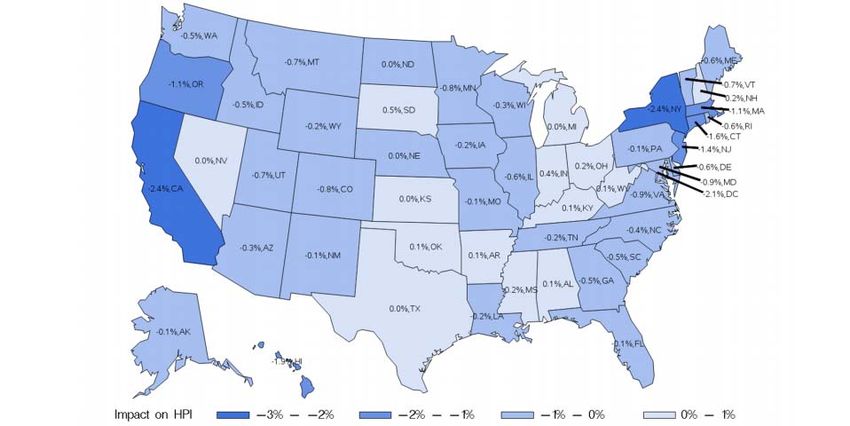
Fed Pressures Short Rates, Inflation Expectations Threaten Long Rates

 Short Rates Reacted to Fed Tightening12
 The Federal Reserve began increasing rates from zero (effectively 0.00% - 0.25%) with one
 25bp rate increase in December 2015, two increases in 2016, and three more in 2017. The Fed “dot
 plot” anticipates three rate increases in 2018 to ~2.0%-2.25% with a further increase to ~2.5%-2.75%
 by YE’19.
 As expected, the front end of the Treasury yield curve reacted to changing policy with 2yr
 Treasury yields increasing from 1.2% to 1.9% during the year.

 Exhibit 2: Fed Funds Effective Rates and the 2yr Treasury Yield

  2.50%                                                                                           2.50%

  2.00%                                                                                           2.00%

  1.50%                                                                                           1.50%

  1.00%                                                                                           1.00%

  0.50%                                                                                           0.50%

  0.00%                                                                                           0.00%
      Aug-16    Oct-16   Dec-16      Feb-17      Apr-17   Jun-17    Aug-17      Oct-17   Dec-17
                                  2yr Treasury            Effective Fed Funds

 Source: Bloomberg, priced on January 11, 2017.

 Long Rates Flattish in 2017, Moving Higher into 2018
 In 2017, 10yr Treasury yields were volatile, but ended the year at 2.4% or 5bp lower than at YE’16,
 with a high of 2.62% and a low of 2.06%.
 Early in 2018, 10yr Treasury yields increased by ~15bp to 2.55% in response to expectations for policy
 driven economic growth in the U.S. pushing inflation expectations higher, along with the Bank of
 Japan reducing their buying of long dated bonds suggesting global QE will be less beneficial to bond
 prices going forward.13

 2018 Rate Outlook: Rising Inflation Expectations Post Tax Reform
 Long-term inflation expectations (measured through 10yr TIPS breakevens) were muted through
 2017, but rapidly increased after the Tax Reform Act passed. 10yr TIPS jumped from 1.9% in mid-
 December to over 2% in early January.14
 Economists at Goldman Sachs and Deutsche Bank expect that the Fed will be increasingly aggressive
 at raising short-term rates over the next 12-24 months as building wage growth places upward
 pressure on overall inflation.

 12 All data from Bloomberg and St. Louis Fed FRED Economic Research.
 13 Bloomberg, “BOJ Tightening to Begin Sooner Than Expected”, January 10, 2018.
 14 TIPS data from Bloomberg, as of January 11, 2018.

PRETIUM PARTNERS | 2018 U.S. Housing Outlook                                                              4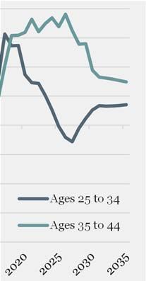
Exhibit 3: U.S. 10yr Inflation Expectations Using TIPS Breakevens

    2.20%
    2.10%
    2.00%

    1.90%
    1.80%
    1.70%
    1.60%
    1.50%

                                             10yr Breakevens

 Source: Bloomberg, priced on January 11, 2018.

 Market Still Not Pricing In Significantly Higher Long-Term Rates
 One issue to watch going forward is how aggressive the Fed can be at pushing up short rates as the
 spread between short and long rates converge. The “2s10s” Treasury yield spread is now just ~55bp.
 Further, the 10yr yield curve remains lower and flatter than a year ago implying that the market is less
 constructive on long-term rate increases despite the recent increase in rates.

 Exhibit 4: 10yr Treasury Yield flattish this year, with the forward curve flattening on weaker
 growth outlook

  2.80%                                            160bp                      10yr Forward Curve
  2.60%                                                        3.60%
                                                   140bp
  2.40%                                                        3.40%
  2.20%                                            120bp       3.20%
  2.00%                                                        3.00%
                                                   100bp
  1.80%                                                        2.80%
  1.60%                                            80bp
                                                               2.60%
  1.40%
                                                   60bp        2.40%
  1.20%
                                                               2.20%
  1.00%                                            40bp
                                                               2.00%
                                                                       Today 6mo    1yr 18mo 2yr   3yr   5yr   10yr

                    2s10s Spread         10yr                                      1yr ago    Current

 Source: Bloomberg, priced on January 11, 2018.

PRETIUM PARTNERS | 2018 U.S. Housing Outlook                                                                          5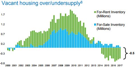
Mortgage Rates Increased Y/Y, Impacting Affordability
 30yr mortgage rates fell from 4.3% at YE’16 to 4.0% at YE’17 due to a contraction in credit spreads
 and a flattening of the long-end of the Treasury curve. While mortgage rates fell from December
 2016, the average in 2017 (4.0%) was higher than 2016 (3.65%) negatively impacting affordability.15
 Historically, rising rates have not had an adverse effect on housing prices as higher rates have
 reflected a stronger economic outlook (and increased the replacement cost for new housing). In the
 near-term, higher mortgage rates are likely to adversely affect affordability and are likely to boost
 rentership.

 Exhibit 5: Freddie Mac 30yr Conforming Mortgage Rate

      7.0%

      6.5%

      6.0%

      5.5%

      5.0%

      4.5%

      4.0%

      3.5%

      3.0%

 Source: Freddie Mac Primary Mortgage Market Survey.

 15   Data on rates from Bloomberg and St. Louis Federal Reserve, data as of December 29 2017.

PRETIUM PARTNERS | 2018 U.S. Housing Outlook                                                             6
Section II: Where Are We in the Housing Cycle?
In our view, the U.S. housing market is characterized by strong demand for housing
above the pace of new construction leading to compressing vacancy rates and declining
levels of for sale housing both of which support higher rents and home prices.
Housing Vacancy Rates Continue to Compress
Housing vacancy rates (per the U.S. Census) are 3.4%, the lowest rate since the early 1990s and down
meaningfully from ~5% in 2009. This contraction is the result of several years of underbuilding new
supply relative to underlying housing demand.
Looking forward, if consensus forecasts for starts of 1.3mn in both 2018 and 2019 (gross, before
obsolescence) prove correct, and household formations rebound to the 1.35mn level projected by
Harvard’s JCHS and Morgan Stanley, then housing vacancy rates would contract by a further 25bp
per year.16 If this happens, by 2019, housing vacancy would be ~3%, the lowest level since the 1980s.
Exhibit 6: Housing vacancy rates, 1965-2017
5.0%
4.5%
4.0%
3.5%
3.0%
2.5%
2.0%
Total Housing Vacancy Rate Historical Average
Source: U.S. Census Bureau, Current Population Survey/Housing Vacancy Survey, Series H-111, through 3Q’17.
To further illustrate this point, Exhibit 7 shows a Freddie Mac analysis looking at the cumulative
supply / demand deficit for vacant and available homes. Since 2008, demand for shelter in the U.S.
has far outpaced new housing supply to the point where we are at a deficit in housing production
versus household formations, especially for rental housing (green bars).
Exhibit 7: Difference Between U.S. Housing Supply and Demand, cumulative
Source: Freddie Mac, Investor Presentation, November 2017.
16 Harvard Joint Center for Housing Studies, “Baseline Household Projections for the Next Decade and Beyond”, December 2016. Morgan Stanley, 2018
Securitized Product Outlook, November 27, 2017.
PRETIUM PARTNERS | 2018 U.S. Housing Outlook 7The U.S. Census data is confirmed by high occupancy rates in the national multi-family market.
According to Axiometrics, occupancy rates for Class B multi-family (defined as the median priced
units in a market) were 95.1%, down 30bp Y/Y. Class A and Class C occupancy rates were also ~95%,
each down 30bp from a year ago.
Exhibit 8: Multi-family Occupancy Rates by Class
97%
96%
95%
Axiometrics expects
94% median multi-family
rent growth of +3.4%
93%
CAGR from 4Q’17 to
92% 2022
91%
90%
Class A Multi-family Class B Multi-family Class C Multi-family
Source: Axiometrics, data as of 3Q’17.
Less Availability Supports Rental Rent Growth
As illustrated below, Axiometrics reports that for the past five years multi-family rental rates have
increased by over 4% per annum. While the rental growth chart for Class A and Class B assets shows
a deceleration over the past 12 months (i.e. +2.3% for class B Y/Y vs. +3.7% a year earlier), this is
largely due to supply pressures and not because of slowing demand.
Longer-term, Axiometrics expects Class B rents will see a +3.4% CAGR from 4Q’17 to 2022.17
Exhibit 9: Multi-family Rents: Class B Rents have recently Outperformed Class A Rents
125
120
115
110
105
100
Class A Multi-family Class B Multi-family
Source: Axiometrics data as of 3Q’17.
17 Axiometrics effective rent growth forecasts, as of 3Q’17.
PRETIUM PARTNERS | 2018 U.S. Housing Outlook 8Alternatively, the Bureau of Economic Analysis’ core personal consumption expenditures data shows
that since 2010, rents have increased at a pace 250bp higher than inflation. The Federal
Reserve relies on the PCE data as an inflation gauge, so both overall PCE and the shelter component
will be important to watch for Fed policy over the next 24 months.
Looking forward, our view is that rental rates should continue to move higher at an above-average
pace barring a setback in the economy or unforeseen increase in new supply.
Exhibit 10: Rental Rate Change: Nominal (line) and Real (bars)
8.0%
6.0%
4.0%
2.0%
0.0%
-2.0%
-4.0%
PCE: Real Rent Growth PCE: Nominal Rent Growth
Source: Bureau of Economic Analysis.
PRETIUM PARTNERS | 2018 U.S. Housing Outlook 9Existing Home Price Appreciation and Inventory
Housing values rose through 2017 due to steady demand growth, rising input costs, and a continued
lack of new housing supply. Demand has been strongest and supply constraints most acute at lower
price points leading to especially strong tailwinds for price appreciation at the lower price segments
(see Exhibit 14 and 15).
CoreLogic estimates that home prices grew 7.0% Y/Y through November 2017 and are now
about 1.2% above their 2006 peak level.18
Case-Shiller estimates that prices in its 20-City Composite Index rose 6.4% Y/Y through
October 2017 and are still 1.7% below their 2006 peak level.19
Per the FHFA Purchase-Only Index, national home prices rose 6.5% Y/Y through 3Q’17 and
are now 10.8% above peak.20
While home prices have recovered well from their post-crisis lows, they remain well off the pace of
multi-family values which are now more than 50% above the prior peak in 2007, having also
recovered about 260% from post-crisis lows.
The sharp growth in multi-family property values has in part supported a strong supply response
from multi-family developers, especially in coastal, Class A markets. This ample supply growth
is an important factor in the decelerating revenue and net operating income (“NOI”) growth of
coastal, Class A apartments.
Exhibit 11: Single-Family Home Price Index and Apartment Price Index
275
250
225 Apartment values
Index 100 = Jan. 2001
are 53% above pre-
200 crisis peak
175 S&P/Case-Shiller
HPI is ~2% above
150 its pre-crisis peak
125
100
75
S&P CoreLogic Case-Shiller 20-City Composite Home Price Index
Moody's/RCA Commerical Property Price Index - Apartment
Source: S&P CoreLogic Case-Shiller 20-City Composite Home Price SA Index as of October 2017; Moody’s/RCA National
Commercial Property Price Index (Apartment) as of October 2017.
18 CoreLogic Home Price Index, Single-Family Combined Tier, as of November 2017. The CoreLogic HPI is built on public
record, servicing and securities real-estate databases and incorporates more than 40 years of repeat-sales transactions. The
“Single-Family Combined” tier includes all sales for single-family attached and detached properties.
19 S&P CoreLogic Case-Shiller 20-City Composite Home Price SA Index, as of October 2017.
20 FHFA Purchase-Only SA Index, as of 3Q’17. The Index is a weighted, repeat-sales index measuring average price changes in
repeat sales on the same properties. This information is obtained by reviewing repeat mortgage transactions on single-family
properties whose mortgages have been purchased or securitized by Fannie Mae or Freddie Mac since January 1975.
PRETIUM PARTNERS | 2018 U.S. Housing Outlook 10Significant Lack of For Sale Inventory
One driver for higher home prices is the lower level of homes for sale, both new and existing, relative
to the pace of demand growth.
In 2017, on average, there were 1.6mn existing homes for sale down 7% from 2016 levels. Further, as
sales activity increased against lower inventory levels, the months’ supply of existing homes for sale
averaged just 3.9 months in 2017, compared to a 6.7 month average from 1985-2016.21
Exhibit 12: Existing Homes for Sale as a % of U.S. Households
3.5%
3.0%
2.5%
2.0%
1.5%
1.0%
0.5%
Existing Home Inventory as a % of HHs
Average Existing Home Inventory as %, 1985-2016
Source: U.S. Census Bureau and National Association of Realtors, Existing Home Sales report through November 2017.
Exhibit 13: Months’ Supply of Existing Homes for Sale
12
10
8
6
3.9
4
2
0
Existing Home Sales Inventory Months Supply
Average Existing Months Supply, 1985-2016
Source: U.S. Census Bureau and National Association of Realtors, Existing Home Sales report through November 2017.
21 U.S. Census Bureau and National Association of Realtors, Existing Home Sales report through November 2017.
PRETIUM PARTNERS | 2018 U.S. Housing Outlook 11Price Growth Stronger Among Lower Price Points
Due to an increased supply of new higher-end homes and lesser production of entry-level homes,
inventory levels among price tiers have diverged substantially.
In Exhibit 14 below, analysis by Zillow shows that even though the absolute inventory level for all
price levels has declined, inventory levels for the middle and bottom tiers have declined ~30% since
January 2015 versus less than 15% for top-tier homes. Although home builders have recently
attempted to increase their focus on the entry-level segment, thus far this has done little for inventory
levels.
Exhibit 14: Change in Inventory by Home Price Tier since Jan-2015
100
Inventory Indexed to Jan-2015
95
90
85
80
75
70
65
60
Bottom Tier Middle Tier Top Tier
Source: Zillow.com, as of October 2017. Seasonally adjusted for-sale inventory. Price tiers based on median estimated home
value within a given region. Bottom-tier homes fall into the bottom third of home values within a given region. Middle-tier
homes fall into the middle third. Top-tier homes fall into the top third.
Due to tightening inventory at lower price points especially, appreciation in the lower price segments
has outpaced the national average and the higher priced segment (see Exhibit 15 below). Looking
forward, the relative out-performance of lower priced homes should continue as long as homebuilders
are unable to build entry-level homes in sufficient numbers.
Exhibit 15: CoreLogic HPI by Purchase Price Segment since Jan-2015
130
HPI Indexed to Jan-2015
125
120
115
110
105
100
High price Middle-to-moderate price Low-to-middle price Low price
Source: CoreLogic, as of November 2017. The four price tiers are based on the median sale price and are as follows: homes
priced at 75 percent or less of the median (low price), homes priced between 75 and 100 percent of the median (low-to-middle
price), homes priced between 100 and 125 percent of the median (middle-to-moderate price) and homes priced greater than
125 percent of the median (high price).
PRETIUM PARTNERS | 2018 U.S. Housing Outlook 12When will HPA Support Additional Entry-Level Housing Starts?
During this housing cycle, median new home sales prices have increased much more and much faster
relative to existing home sales prices. Year-to-date through November 2017, the difference between
new and existing home sales prices was 32%, or more than double the 14% average spread since 1980.
Historically, a 10-15% spread has been warranted, as newer homes tend to be larger and have more
modern features and amenities than older existing homes.
Exhibit 16: Median New and Existing Home Sales Prices
$350
YTD Pricing Trends
$300 New Home Median Px = $317k
Exist. Home Median Px = $248k
$250 Current ∆ = 28% ∆ Since 1980 = 18%
$200
$150
$100
$50
$0
1980 1985 1990 1995 2000 2005 2010 2015
Existing Home Sales, Median Sales Price New Home Sales, Median Sales Price
Source: U.S. Census Bureau, Median Sales Price of Houses, as of November 2017; U.S Census Bureau and U.S Department of
Housing and Development, Median Sales Price for New Houses Sold, as of November 2017.
The two drivers of higher new home prices are increasing per square foot costs, as well as increasing
new home sizes. The selling price of new homes has increased rapidly since 2011 from $98/sf to over
$130/sf. The median size of a new home sold in the U.S. was ~2,400sf in 2017. The median size has
fallen by 4% over the past two years, but remains 17% above the median size in 2000.
Exhibit 17: Median Size and Price per square foot of New Home Sales
$140 $131 2,600
$130
2,500
$120
$110 $98
2,400
$100 $78
$90 2,300
$80
2,200
$70
$60
2,100
$50
$40 2,000
Median New Sales Price PSF (lhs) Median New Sales, Home Size (rhs)
Source: U.S. Census Bureau, Median Sales Price of Houses, as of November 2017. Median Size of New Homes Sold, data
through 3Q’17.
PRETIUM PARTNERS | 2018 U.S. Housing Outlook 13Section III: Housing Fundamentals: Current and Outlook
Demand Trends: 2017 below Expectations but Long-Term Drivers Intact
Year-to-date through September 2017, the U.S. created 754k new households, which was a slowdown
from the 950k households formed in 2016 and 1.35mn formed in 2015. Over the next several years,
Harvard’s JCHS expects household formation to average 1.36mn per annum from 2016-2025, so
growth in 2017 has been below expectations.22
Housing observers, including Harvard’s JCHS, Morgan Stanley’s Housing Strategy team, and Stephen
Kim at Evercore-ISI, argue that while the household formation numbers have been weaker than
expected, constructive demographics and positive Millennial employment / wage growth trends
should combine for a more normal pace of household formation going forward. Morgan Stanley
argues for 1.3-1.35mn household formations per annum over the next five years, while Evercore-ISI
forecasts 1.50mn household formations in each of 2018 and 2019.23
Exhibit 18: Annual Household Formations, with Harvard’s JCHS Forecasts
2,000
1,800
1,600
1,400
1,200
1,000
754
800
600
400
200
0
Household Formations Harvard's JCHS Projections Average HH Formations, 1990-2006
Source: U.S. Census Bureau, Household Formations Tables 13 and 13a. Projections from Harvard JCHS, “Baseline
Household Projections for the Next Decade and Beyond”, December 2016.
Favorable Demographics Drive Demand Outlook
The Millennial generation has overtaken the Baby Boomers in total population and is the largest
generation in American history with 83mn people aged 16-34 in 2016. The ageing of the
Millennials into adulthood is the most significant demographic event taking place today
and, for the next 20 years, is expected to have broad economic impacts similar in
magnitude to those of the Boomers.24
As the Millennial generation ages over the next decade, growth in the 35 to 44 year old cohort will be
outpaced only by the 65+ cohort. As the propensity to live in single-family housing increases as people
age into their 30s and 40s, this cohort should contribute significantly to demand growth for single-
family housing, both owner and renter occupied.
22 Harvard JCHS, “Baseline Household Projections for the Next Decade and Beyond”, December 2016.
23 Morgan Stanley, 2018 Securitized Product Outlook, November 27 2017. Evercore-ISI, “Salad Days”, January 3, 2018.
24 U.S. Census report, “Millennials Outnumber Baby Boomers and Are Far More Diverse” June 2015.
PRETIUM PARTNERS | 2018 U.S. Housing Outlook 14Population Shifts a Long-Term Driver of Household Formations
The 2017 slowdown in housing demand occurred despite robust population growth in the young adult
age cohorts, with ~70mn Americans between the ages of 20 to 35 entering the prime household
forming years.25 This is the demographic underpinning of the above-average housing demand
forecasts from Harvard’s JCHS and Morgan Stanley.
Exhibit 19: Population Shifts Support Return to Above-Average HH Formation Growth
25 80%
22.7 22.4 22.3
23 21.1 21.6 21.8
70%
21
The % of people
60% leading a
U.S Population (mn)
19
50% household jumps
17 from 30% at 20 to
15 40% 24 years old to
13 30% almost 50% in the
11 30 to 34 cohort
20%
9
7 10%
5 0%
Population Headship Rate
Source: Morgan Stanley U.S Housing Strategy, “Demand, Supply and Housing Policy,” February 2017.
Shown another way, Moody’s Analytics forecasts that from 2015 to 2035 the 35 to 44 year old cohort
will increase by 12mn people or 30%. This growth will be well above the growth in the 25 to 35 year
old population, which supported above-average multi-family fundamentals over the past decade.26
Exhibit 20: Population Growth, Ages 35 to 44 Exhibit 21: Annual Population Growth
55 2.0%
Ages 35 to 44 (millions)
1.5%
50 1.0%
0.5%
45 0.0%
-0.5%
40 -1.0%
Ages 25 to 34
-1.5%
Ages 35 to 44
35 -2.0%
Source: U.S. Census Bureau and Moody’s Analytics.
25 Morgan Stanley U.S Housing Strategy, “Demand, Supply and Housing Policy,” February 2017.
26 Moody’s Analytics. Population forecast as of December 2017.
PRETIUM PARTNERS | 2018 U.S. Housing Outlook 15Will Millennial Employment Growth Unlock Pent Up Demand?
Employment of younger cohorts has been growing quickly since the end of the last recession.
According to the Bureau of Labor Statistics, employment of the 20 to 24 and the 25 to 34 age cohorts
increased by nearly 6.2mn since 2010, representing approximately 35% of all net employment growth.
The unemployment rate for the 18 to 24 and 25 to 34 age cohorts fell to 5.1% and 3.9%, respectively,
as of November 2017.27 This compares to an overall unemployment rate of 4.1%.28
Continued strong employment prospects for these age groups should continue to drive household
formations. Young people confident with their employment are more likely to form households, move
into new homes, and create families.
This is increasingly important, as the number of young people living at home has hit all-time highs.
Most concerning is the number of 25 to 34 year olds living at home. From 2003 to 2017, the
percentage of people in this cohort living at home increased from 10.2% to 16.1%, an increase of over
3.1mn people. At two to three persons per household, this equates to ~1.0mn to ~1.5mn households
of pent-up demand.
Exhibit 22: Share of Young Adults Living with Parents has Increased Sharply since the Recession
58% 18%
16.1%
56% 16% Unlike most charts
in this report, the
54% 14% lines moving up
and to the right is a
54.8% bad thing.
52% 12%
More young adults
50% 10%
are staying at home
10.2% due to preference or
48% 49.5% 8%
inability to move
out and form
46% 6% households.
44% 4%
18 to 24 years old 25 to 34 years old
42% 2%
1975
2015
1960
1970
1980
1990
2000
2010
1965
1985
1995
2005
2010
1975
2015
1960
1970
1980
1990
2000
1965
1985
1995
2005
Source: U.S. Census Bureau, Current Population Survey, March and Annual Social and Economic Supplements. Source of
1980, 1970, and 1960 data: U. S. Bureau of the Census, 1980 Census of Population, PC80-2-4B, "Persons by Family
Characteristics," table 4. 1970 Census of Population, PC(2)-4B, table 2. 1960 Census of Population, PC(2)-4B, table 2.
27 U.S. Bureau of Labor Statistics, Unemployment rates by age, sex, and marital status, seasonally adjusted, November 2017.
28 U.S. Bureau of Labor Statistics, Civilian Unemployment Rate, seasonally adjusted, November 2017.
PRETIUM PARTNERS | 2018 U.S. Housing Outlook 16Sun Belt Benefitting from Outsized Employment and Population Growth
Citing national population growth figures ignores one of the other significant demographic events
happening today – the continued shift of the U.S. population to southern cities and states.
As William Frey of Brookings has written about extensively, in both cities and suburbs, post-recession
population growth in the Sun Belt (Southeast and Southwest) is well above the positive but
decelerating growth in the Snow Belt (Midwest and Northeast). From 2015 to 2016, year-on-year
growth in Sun Belt cities and suburbs was over 1.2%, while growth in the Snow Belt was ~0.2%.29
Below we look at the MSAs with the strongest and weakest migration flows growth from 2015 to 2016.
Population growth from in-migration (both domestic migration and immigration) was dominated by
metro areas like Dallas, Houston, Phoenix, Tampa, Atlanta, and Seattle. On the other end of the
spectrum, metro areas such as Chicago, New York, Los Angeles, Milwaukee, and Detroit saw net out-
migration.30
Looking forward, we continue to expect above-average population growth in fast-growing Sun Belt
markets, which will support above-average employment growth as companies are able to access
significant pools of quality labor in markets with more affordable living costs for employees.
Exhibit 23: Metros with the most and least beneficial net migration flows, 2015-2016
Net Migration 2015-2016 (thousands)
-75 -50 -25 0 25 50 75 100
Dallas
Houston
Phoenix
Tampa
Atlanta
Seattle
Miami
Orlando
Austin
Charlotte
Las Vegas
San Antonio
Portland
Denver
Metro Area
Nashville
Jacksonville
Raleigh
Riverside
Sarasota
Cape Coral
Virginia Beach
Memphis
Honolulu
Cleveland
St. Louis
Detroit
Milwaukee
Los Angeles
New York
Chicago
Source: U.S. Census Bureau, Estimates of the Components of Resident Population Change: April 1, 2010 to July 1, 2016 and
Annual Estimates of the Resident Population: April 1, 2010 to July 1, 2016. Release Date: March 2017.
29 William Frey, Brookings Institute. https://www.brookings.edu/blog/the-avenue/2017/05/30/city-growth-dips-below-
suburban-growth-census-shows/, and https://www.brookings.edu/blog/the-avenue/2017/03/30/census-shows-a-revival-of-
pre-recession-migration-flows/.
30 U.S. Census Bureau, Estimates of the Components of Resident Population Change: April 1, 2010 to July 1, 2016 and Annual
Estimates of the Resident Population: April 1, 2010 to July 1, 2016. Release Date: March 2017.
PRETIUM PARTNERS | 2018 U.S. Housing Outlook 17Supply Trends: Slowly Increasing, Need More Starter Homes
Year-to-date through November 2017, new housing starts averaged 1.21mn at a seasonally adjusted
annual rate (“SAAR”), up from 1.18mn in 2016 and 1.11mn in 2015. Average new starts from 1980-
2006 were over 1.5mn units, so while new home construction has picked up it remains well below
“normal” levels.
Exhibit 24: Total Housing Starts 1.21mn in 2017, up from 1.18mn in 2016
2,500
2,000
1,500
1,000
500
0
1980 1983 1986 1989 1992 1995 1998 2001 2004 2007 2010 2013 2016
Single Family Housing Starts (000s) Multi-Family Housing Starts (000s)
Source: U.S. Census Bureau and U.S. Department of Housing and Urban Development, New Residential Construction, New
Privately-Owned Housing Units Started. Latest data through November 2017.
Starts Outlook – Continued Single Digits Growth
Looking forward, consensus forecasts housing starts of 1.27mn in 2018 and 1.32mn in
2019 (see Exhibit 25 below), which would equate to growth of 6% and 3%, respectively.31
Exhibit 25: U.S. Housing Starts Forecasts
2017 e 2018e 2019e
Starts (in 000s)
Fannie 1 ,1 9 7 1 ,2 55 1 ,3 05
Freddie 1 ,2 00 1 ,3 00
MBA 1 ,1 9 5 1 ,2 89
Zelm an 1 ,2 1 0 1 ,2 95 1 ,3 50
Goldm an Sachs 1 ,1 9 6 1 ,2 55 1 ,2 90
Morgan Stanley 1 ,2 01 1 ,2 2 3 1 ,3 3 7
Av erage 1,200 1,27 0 1,321
Y/Y 2.2% 5.8% 4.0%
Source: Latest forecasts as of January 3, 2017.
31 Consensus forecasts are a simple average of the latest forecasts from Fannie Mae, Freddie Mac, MBA, Zelman & Associates,
Goldman Sachs, and Morgan Stanley.
PRETIUM PARTNERS | 2018 U.S. Housing Outlook 18Exhibit 26 illustrates that while housing starts are increasing, relative to the size of the population,
housing starts by 2019 will be back only to 1991 levels, a period of a severe real estate
recession.
Exhibit 26: Housing Start Forecasts as a % of Population Remain Depressed
0.8% 2,000
0.7% 1,800
Start as & of U.S. Population
1,600
0.6%
Total Housing Starts
1,400
0.5% 1,200
0.4% 1,000
0.3% 800
600
0.2%
400
0.1% 200
0.0% 0
1980 1985 1990 1995 2000 2005 2010 2015
Total Housing Starts Starts as % of US Population
Source: Historical housing starts from U.S. Census Bureau, as of December 2017. Housing starts forecasts from Exhibit 21.
Historical and forecasted population from U.S. Census Bureau.
Freddie Mac and Harvard’s JCHS argue that the current pace of housing construction is between
400-500k units less than what is needed to house incremental households and replace obsolete
and ageing stock.32
Researchers at Harvard’s JCHS added that, “Given that current construction levels are so far below
baseline demand levels, future completions and placements in 2015-2025 will likely be well below our
baseline demand estimates for that period unless construction levels ramp-up sharply in the next few
years.”33
Exhibit 27: Housing Completions below Long-Term Demand / Replacement
2,500 Harvard's JHSC Housing Demand Forecast =
1.7mn /yr from household formations and obsolescence
2,000
1,500
2017 Deficit
1,000
500
1980 1983 1986 1989 1992 1995 1998 2001 2004 2007 2010 2013 2016 2019 2022 2025
Total Housing Completions + MH Deliveries (000s)
Average Total Housing Production (1980-2005)
Harvard JCHS Baseline Annual Demand Estimate, 2015-2025
Source: Harvard Joint Center for Housing Studies, Baseline Household Forecasts, December 2016.
32 Source: U.S. Census Bureau, HUD Components of Inventory Change report, National Association of Home Builders, Freddie
Mac, “Can We Spot the Next House Price Bubble”, November 2017.
33 Harvard Joint Center for Housing Studies, Baseline Household Forecasts, December 2016.
PRETIUM PARTNERS | 2018 U.S. Housing Outlook 19Construction Deficit Includes a Shortage of Entry-Level Housing
In addition to an underbuilding of shelter broadly, there is a growing shortage of entry-level
housing in particular. Homebuilders have produced larger, more expensive homes than what
builders offered pre-recession.
The main reasons for this are higher fixed costs that necessitate building higher priced homes to
achieve profitability and post-crash builders that are focused on move-up and more affluent buyers
who are more easily able to obtain mortgages.
Net, there are fewer starter / entry-level homes – today and over the past decade – being produced for
a growing pool of ageing Millennials who are moving through life events (marriage, children, etc.) and
now need more space to raise their families.
In 2016 (latest data available), builders started construction on only 362k homes under 2,400 square
feet. In comparison, between 2005 and 2007, the U.S. produced over 900k such units each year.
Exhibit 28: Single-Family Housing Starts for Units below 2,400 square feet
1,000 949
900
800
700
600
500
362
400
300
200
100
0
SF Home Completions < 2,400 sq. ft.
Average Completions, 1990-2006 < 2,400 sq. ft.
Source: U.S Census Bureau, New Privately Owned Housing Units Completed, Square Feet of Floor Area in New Single-
Family Houses Completed. Annual data, 1968-2016.
This shortage of entry-level homes is also evident in the new home sales data. In 2017, only 14% of
new homes purchased were sold for under $200k, compared to 39% in 2005. Similarly, in 2017, 45%
of new homes sold were below $300k, compared to 66% in 2005.34
34 U.S. Census Bureau, “Monthly New Residential Construction, November 2017,” December 19, 2017. Data through November 2017.
PRETIUM PARTNERS | 2018 U.S. Housing Outlook 20Homeownership Rate Stabilizes, but Credit Availability and Stressed
Balance Sheets Remain a Headwind
The homeownership rate stabilized in the high 63% range during 2017, after more than ten years of
declines from the 2004 peak of 69%.
Exhibit 29: U.S. Homeownership Rate, 1965-2017
70%
69%
68%
67%
66%
65%
64%
63%
62%
61%
60%
Homeownership Rate Average, 1965-2017
Source: U.S. Census Bureau, Current Population Survey/Housing Vacancy Survey, Series H-111, as of 3Q’17. Released:
October 31, 2017.
Within age cohorts, the homeownership rate for the under 35 and 35 to 44 age cohorts saw the most
noticeable stabilization, although these age cohorts saw the greatest decline over the past decade of
800bp and 1,000bp, respectively.
Looking forward, we expect these cohorts will struggle to increase homeownership rates given the
macro constraints of tighter mortgage credit availability and the impact on personal balance sheets
from student and other non-mortgage debt loads.
Exhibit 30: U.S. Homeownership Rate by Age Cohort, 1982-2017
90%
80% 65 years and over
70% 55 to 64 years
45 to 54 years
60%
35 to 44 years
50%
Under 35 years
40%
30%
< 35 y ears 35 to 44 y ears 45 to 54 y ears 55 to 64 y ears > 65 y ears U.S.
2 004 4 3 .1 % 69.2 % 7 7 .2 % 81 .7 % 81 .0% 69.0%
2 01 7 3 5.1 % 59.0% 69.3 % 7 5.3 % 7 8.6% 63.7 %
Δ -800bp -1020bp -7 90bp -64 0bp -2 4 0bp -530bp
Source: U.S. Census Bureau, Current Population Survey/Housing Vacancy Survey, Series H-111, as of 3Q’17. Released:
October 31, 2017.
PRETIUM PARTNERS | 2018 U.S. Housing Outlook 21Consumer Balance Sheets Increasingly Levered with Non-Mortgage Debt
One potential headwind to future homeownership is the increased student and other non-mortgage
debt burden of younger cohorts post-recession. In our view this debt negatively impacts the ability to
save for a down payment and afford monthly mortgage payments given the additional interest
expense burden.
According to the New York Fed, since 3Q’08 the U.S. households have added $750bn of student debt,
or $6,000 more per U.S. household. Overall, U.S. consumers have added $1.2bn of auto, student, and
credit card debt since 2008, while mortgage debt has fallen by $800bn. The average household has
$28,400 of auto, student, and credit card debt, up 39% from Q3’08.35
Exhibit 31: Change in Components of U.S. Consumer Debt, 3Q’08-Present
$1.5 $1.2
$1.0
$0.5
$0.0
$ Trillion
-$0.5
-$1.0
($0.80)
-$1.5
-$2.0
∆ Mortgage Debt since 3Q'08 ∆ Auto and Student Debt since 3Q'08
Source: Federal Reserve Bank of New York, Quarterly Report on Household Debt and Credit, as of 3Q’17.
Focus on Student Loans
“Among younger
From 2004 to 2015, student loan balances (average, per borrower) increased from borrowers, the
$15,300 to $26,700 for borrowers under 40 years old. Not only are the averages per ballooning of student
debt may have
borrower increasing, but so are the numbers of borrowers – in 2004 there were 17mn substantial spillover
Americans under 40 with student loans, which increased to 29.4mn (+73%) by 2015. effects on their
propensity and ability to
Exhibit 32: Student Loans: # of Borrowers and Average Balances, under 40yrs old take out new mortgages
and auto loans, and it
may postpone other
Borrowers Under US Population, % with Student Average
types of consumption as
40yrs (mn) 20-40yrs (mn) Loans Balance it drives young
2004 17.0 81.0 21% $15,300 borrowers home to live
2006 19.7 81.4 24% $17,700 with their parents.”
2008 22.3 82.2 27% $20,200
2010 25.7 83.0 31% $21,600 – NY Fed, “Greying of
American Debt”
2012 26.0 84.2 31% $24,600
2014 29.2 85.8 34% $25,700
2015 29.4 86.5 34% $26,700
Source: Federal Reserve Bank of New York Consumer Credit Panel / Equifax, “2016 Student Loan Update”.
35 Federal Reserve Bank of New York, Quarterly Report on Household Debt and Credit, as of 3Q’17. Released November 2017.
PRETIUM PARTNERS | 2018 U.S. Housing Outlook 22Mortgage Credit Remains Tight Despite Loosening on the Margin
Along with weaker balance sheets, another major challenge for the housing market has been a slow
normalization of mortgage credit availability post-crisis.
Exhibit 33 (below) from the Urban Institute illustrates the amount of default risk taken by lenders in
new purchase originations. The Urban Institute’s analysis shows no improvement in risk taken by the
mortgage market on new loans post-crisis.
Exhibit 33: Urban Institute Housing Credit Availability Index, 1Q’99 to 2Q’17
20%
Reasonable Total default risk
18%
lending
16%
standards
14%
12% Product risk
10%
8%
6%
4% Borrower risk
2%
0%
Source: eMBS, CoreLogic, Home Mortgage Disclosure Data (HMDA), Inside Mortgage Finance (IMF), and Urban Institute.
Index as of 2Q’17. Updated October 12, 2017.
Tight lending conditions are shown in the average credit score on new purchase originations
from Fannie Mae / Freddie Mac (GSE loans) and the FHA/VA. Relative to pre-crisis levels, average
credit scores on GSE loans are ~+30bp and ~+40bp for FHA loans.
Exhibit 34: FICO at Origination for GSE and FHA Purchase Mortgage Scores since 2005
Source: Black Knight, eMBS, Goldman Sachs Global Investment Research. Goldman Sachs, “Housing and Mortgage Monitor
December 2017 – Homebuilder, homebuyer confidence remain high,” December 19, 2017.
PRETIUM PARTNERS | 2018 U.S. Housing Outlook 23Recent Trends in Mortgage Availability – DTIs Increasing, FICOs Flat
There continue to be marginal improvements to credit availability within both conventional (Fannie
Mae and Freddie Mac) and Ginnie Mae (FHA/VA) loans, primarily on the debt to income ratios of
these loans.
Through October 2017, the trailing 12-month FICO for conventional loans was 751, in-line with the
2016 average and one point below the 2015 average. Similarly, for FHA/VA loans, the average FICO
on a trailing 12 month basis was 694, in-line with both the 2016 and 2015 averages.
Where we see mortgage credit underwriting loosening is on the debt-to-income (“DTI”) ratios for
borrowers. The DTIs capture both the monthly mortgage payment as well as any fixed charges from
other debt (interest + amortization).
For Fannie / Freddie loans, the average DTI in 2017 was 35.3% up from 34.6% in 2016 and 34.4% in
2015. Similarly, the average DTI for FHA/VA loans was 41.8% in 2017 compared to 40.8% in 2016
and 40.4% in 2015. As a reminder, while the Qualified Mortgage (“QM”) rule prohibits loans with
DTI above 43%, any loan purchased by Fannie / Freddie or guaranteed by the government through
the FHA/VA are exempt from QM.
Exhibit 35: GSE and FHA Average Purchase Mortgage FICO and DTI since 2015
760 40% 700 45.0%
43.0%
41.0%
755 35% 695
39.0%
37.0%
750 30% 690 35.0%
33.0%
31.0%
745 25% 685
29.0%
27.0%
740 20% 680 25.0%
Conventional Loans: TTM Avg FICO Ginnie Loans: TTM Avg FICO
DTI DTI
Source: Morgan Stanley, “U.S. Housing Tracker, November 2017,” EMBS.
PRETIUM PARTNERS | 2018 U.S. Housing Outlook 24Potential Regulatory and Policy Impacts on Housing and Credit Availability Tax Reform Act likely to reduce incentive to own and disproportionately impact high- cost markets The Tax Reform Act significantly reduces the incentive to itemize deductions by doubling the standard deduction to $12k for a single person and $24k for a married couple and increasing the child tax credit to $2k. In sum, this would limit the value of itemizing deductions, which would be further limited by capping the mortgage interest deduction to loan principle below $750k, down from $1mn today, and capping total state, local, and property taxes deductions to $10k. Preliminary analysis of early proposals of the plan by Stephen Kim at Evercore-ISI predicted that only those making well over $200k would itemize under the new tax plan; others would choose the increased standard deduction instead.36 Therefore a buyer of median priced home would likely face zero tax incentive for owning versus renting under the new tax plan because they would not elect to itemize. As analysts from Morgan Stanley put it, “the trickiest aspect of this is homeowners in the middle. While the mortgage interest deduction is not going away, a doubling of the standard deduction combined with a $10k cap on state and local property deductions…means that it will no longer be in the best interest of a lot of households to itemize deductions. A household that does not itemize deductions is no longer receiving an incentive to own a home versus rent.”37 However, the larger standard deduction should benefit lower income tax payers putting more money in their pockets for paying rent, saving for down payments, or making mortgage payments. The tax plan, therefore, should be a positive for entry-level home prices and rents, while potentially negatively impacting higher-end real estate due the limitations of itemized deductions. As shown below in Exhibit 36, analysis from J.P. Morgan shows that the impact to HPA from the tax plan should be limited for the most part to high-cost and high-tax states including California, Oregon, and the Northeast, while having nearly zero impact in the rest of the country. Exhibit 36: Estimated Impact of Tax Reform on HPA Due to Removal/Limitation of Deductions Source: J.P. Morgan, “The impact of tax reform on the housing market,” November 22, 2017. 36 Evercore-ISI, “Tax Plan Delivers a Blow to the MID-section,” November 3, 2017. 37 Morgan Stanley, “Agency MBS Weekly: Can You Pay My Bills? Pay My Deductible?” November 3, 2017. PRETIUM PARTNERS | 2018 U.S. Housing Outlook 25
After tax reform, Congress may finally take up GSE reform in 2018
 With their first major legislative accomplishment and tax reform out of the way, Republican
 Congressional leaders may turn their attention to GSE reform in 2018, just as Fannie and Freddie
 capital levels reach concerning levels.
 Several potential GSE reform solutions have been proposed and debated by think tanks and lobbying
 groups, but House Financial Services Committee Chairman Jeb Hensarling (R-TX) spoke in early
 December indicating his support for a plan resembling the Bright-DeMarco proposal after accepting
 that passage of his PATH Act was unlikely. Hensarling now supports an explicit government
 guarantee, a complete wind-down of the GSE’s, and expanding private capital involvement in the
 market.
 Under the plan, the Ginnie Mae securitization platform would provide a government backstop for
 mortgages. Ginnie Mae would become a standalone corporation that would be able to issue securities
 with private mortgage insurance credit enhancements as well as loans guaranteed through the FHA
 and the VA.
 However, there is less support in the Senate for major changes, with more moderate Republican
 Senators open to leaving Fannie and Freddie unchanged.

 Financial deregulation proposed by Treasury could reduce bank demand for
 mortgage backed securities
 The Treasury released three reports this year providing recommendations to change regulations
 pertaining to banks and capital markets. In particular, it proposed changes to bank capital rules and
 to the securitization market that could reduce bank demand for mortgage backed securities. Some
 adoption is likely, as these changes would not require legislation and can be expected to be
 incorporated into regulatory rule-making in 2018.
 In addition to recommending that highly rated securitized debt be treated the same way as IG-rated
 corporate debt for Liquid Coverage Ratio (“LCR”), the Treasury also recommends exempting mid-tier
 banks with $50-$250bn in assets from LCR requirements entirely. Exempting these banks may result
 in an unwinding of their current Ginnie Mae mortgage-backed security (“MBS”) holdings that have
 been bought to meet LCR requirements, lowering overall bank demand for MBS.38
 Further, the Treasury recommends removing cash on deposit, treasuries, and initial margin for
 cleared derivatives from the denominator of the Supplemental Leverage Ratio (“SLR”), which would
 make treasuries look cheaper to hold capital against instead of Ginnie Mae MBS, again reducing bank
 demand for Ginnies.
 As the Federal Reserve unwinds its balance sheet in 2018, the private market will need to absorb a
 much larger net supply of MBS than usual. Banks have absorbed $100-200bn of MBS per year since
 2015. Therefore, regulatory changes that could affect their appetite for Ginnies could have significant
 effects on the MBS market in 2018.

 38   Morgan Stanley, “2018 Global Securitized Products Outlook: Cherry Picking”, November 27, 2017.

PRETIUM PARTNERS | 2018 U.S. Housing Outlook                                                               26
Important Disclosures
 This report discusses general market activity, industry or sector trends, or other broad-based
 economic, market or political conditions and should not be construed or relied upon as research or
 investment advice, as predictive of future market or investment performance or as an offer or
 solicitation of an offer to buy or sell any security or investment service. This report reflects the views
 of Pretium Partners, LLC (“Pretium”), as of the date on the cover and these views are subject to
 change without notice as the market conditions change and evolve, which can occur quickly. Past
 performance is not indicative of future results.
 Recipients are urged to consult with their financial advisors before making any investment. All
 investments entail risks, and mortgage-related investments are speculative and entail special risks.
 Changes in interest rates, both real estate and financial market conditions, the overall economy, the
 regulatory environment and the political environment can affect the market for mortgage-related
 investments and should be considered carefully. Investors may lose all or substantially all of an
 investment, and no investment strategy or process is guaranteed to be successful or avoid losses.
 Certain information in this report has been obtained from published and non-published sources
 prepared by third parties, which, in certain cases, have not been updated through the date hereof.
 While such information is believed to be reliable, Pretium has not independently verified such
 information, does not assume any responsibility for the accuracy or completeness of such information
 nor does it warrant that such information will not be changed.
 The information included herein may not be current and Pretium has no obligation to provide any
 updates or changes. No representation, warranty or undertaking, express or implied, is given as to the
 accuracy or completeness of the information or opinions contained herein, and nothing in this report
 should be relied upon as a promise or representation.
 The information set forth in this report is not intended as a representation or warranty by Pretium or
 any of its affiliates as to the composition or performance of any future investments. Assumptions
 necessarily are speculative in nature. It is likely that some or all of the assumptions set forth or relied
 upon in this report will not materialize or will vary significantly from any assumptions made (in some
 cases, materially so). You should understand such assumptions and evaluate whether they are
 appropriate for your purposes. Certain information in this report is based on mathematical models
 that calculate results using inputs that are based on assumptions about a variety of future conditions
 and events. The use of such models and modeling techniques inherently are subject to limitations. As
 with all models, results may vary significantly depending upon the value and accuracy of the inputs
 given, and relatively minor modifications to, or the elimination of, an assumption, may have a
 significant impact on the results. Actual conditions or events are unlikely to be consistent with, and
 may differ materially from, those assumed. ACTUAL RESULTS WILL VARY AND MAY VARY
 SUBSTANTIALLY FROM THOSE REFLECTED IN THESE MATERIALS.
 Any discussion in this report concerning the U.S. Tax Cuts and Jobs Act of 2017 (the “Tax Reform
 Act”) is preliminary only. This report is not, and should not be construed or relied upon as, tax advice
 or a comprehensive analysis of the Tax Reform Act.
 This report contains forward-looking statements, which can be identified by the use of forward-
 looking terminology such as “may,” “will,” “should,” “seek,” “expect,” “anticipate,” “project,”
 “estimate,” intend,” continue,” “target,” “plan,” “believe,” the negatives thereof, other variations
 thereon or comparable terminology and information that is based on projections, estimates, and
 assumptions. Such statements and information cannot be viewed as fact and are subject to
 uncertainties and contingencies. Actual results during the period or periods covered by such
 statements and information may differ materially from the information set forth herein, and no
 assurance can be given that any such statement, information, projection, estimate, or assumption will
 be realized or accurate.

PRETIUM PARTNERS | 2018 U.S. Housing Outlook                                                                   27
For questions or comments on this report, please contact:

 George Auerbach
 Director – Research & Strategy
 gauerbach@pretiumpartnersllc.com

 Piotr Kopacz
 Associate – Research & Strategy
 pkopacz@pretiumpartnersllc.com

PRETIUM PARTNERS | 2018 U.S. Housing Outlook                 28
You can also read