Analysis of Consumer Demand for American Sports Leagues
←
→
Page content transcription
If your browser does not render page correctly, please read the page content below
Claremont Colleges
Scholarship @ Claremont
CMC Senior Theses                                                                                                  CMC Student Scholarship

2018

Analysis of Consumer Demand for American
Sports Leagues
Sam Healy

Recommended Citation
Healy, Sam, "Analysis of Consumer Demand for American Sports Leagues" (2018). CMC Senior Theses. 1921.
http://scholarship.claremont.edu/cmc_theses/1921

This Open Access Senior Thesis is brought to you by Scholarship@Claremont. It has been accepted for inclusion in this collection by an authorized
administrator. For more information, please contact scholarship@cuc.claremont.edu.
Claremont McKenna College

Analysis of Consumer Demand for American Sports Leagues

                    To be submitted to
                   Professor Vossmeyer
                           and
                     Professor Pedace

                           By,

                       Sam Healy

                            For
                      Senior Thesis
                       Spring 2018
                      April 23, 2018
2
ABSTRACT

Long before the first pitch is thrown, the first snap is taken or the first puck is dropped,
organizations in the professional sports industry set their ticket prices. The secondary ticket
market, on the other hand, has grown into a billion dollar industry and gages the consumer’s
true willingness to pay. This study examines the myriad of factors that influence the
secondary market ticket price of a professional sports game across the MLB, NFL, NBA,
and NHL during the 2013-2014 regular season. Using median ticket prices from a
secondary market ticket aggregator, the results indicate that weekend games and the
expected quality of the away team significantly impact median ticket price. If the game is
played during the last month of the season, median ticket prices decrease by 17%, unless
the home or away team was a playoff team the year before. Furthermore, games that include
a home team where one or two players are among the top ten in jersey sales are associated
with higher median ticket prices.

                                                                                             3
Table of Contents
I. Introduction ……………………………..…………………………… 5
II. Literature Review…………………………………..………………… 9
III. Data……………………………………………………...…………… 14
IV. Method.……………………………………………….……………… 20
V. Results………………………………………………...……………… 22
VI. Conclusion…………………………………………......………...…… 35
VII. References …………………………………………………………… 38
VIII. Appendix …………………………………..………………………… 40
4I. INTRODUCTION
The secondary ticket market for live events has increased dramatically in the last
decade. With consistent growth since the early 2000’s, the secondary ticket market is
estimated to be worth about $15 billion, according to Sports Marketing Quarterly (2017).
Major firms in the market have experienced the same growth. As of 2013, Stubhub has
their name on a 27,000 seat professional sports stadium in Santa Clara, CA. Ticketmaster
and Stubhub have both developed huge partnership deals with the NFL, NBA, NHL and
MLB. The partnerships give these companies the rights to sell and resell the league’s
primary and secondary market tickets and serve as the official ticket marketplace for the
professional franchises. As a result, the online secondary ticket market has become the
ideal place for a fan to visit when s/he is looking to attend a live sporting event.
As time passes, the product that is expected to go onto the playing field, court, or
rink changes. Players can get hurt during the days leading up to the game, lineups can
change to where your favorite player is now delegated to the bench, and even the weather
forecast is a factor that affects fan’s expectations of the quality of the game. As the product
changes, the demand for it and its value in the eyes of the consumer naturally changes as
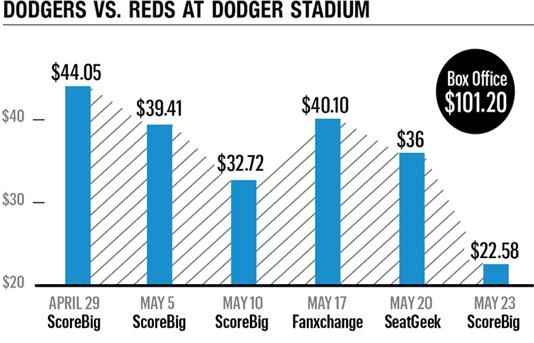
well, as demonstrated in Figure 1. According to consumer reports, as an event draws near,
the ticket prices for a particular seat can experience a great deal of fluctuation.
5Figure I: graph from consumerreports.org highlighting the fluctuating secondary market ticket
prices for an MLB game depending on the date
The quality of play, during the length of an entire season, will vary enormously
from game to game. Some games are inherently more popular than other games because of
a rivalry or a certain players’ celebrity. As a result, each game should be viewed as a unique
product. Professional franchises have to set their ticket prices months before the season
begins. They look at every seat within their stadium and assign it a face value for that
season. No one can predict what the demand will be for a game three-quarters of the way
into a season. For a fan, the face value is often not the same as the ticket value. That is
where the secondary ticket market enters the equation. It capitalizes on an organization’s
inability to predict the future and provides a forum where buyers and sellers agree upon a
thoughtful price minutes before tip-off. The secondary market reveals at what time and cost
people will buy and sell tickets for a particular game, whereas the primary ticket market
does not. Companies, like the two previously mentioned, make it relatively painless to both
buy and sell tickets on their websites. Thousands of buyers and sellers converge on these
secondary ticket market online platforms, making transactions from the moment the tickets
are released up until the moment the game ends. There are hundreds of secondary market
6platforms that offer a wide variety of tickets at a wide variety of prices. Thus, the secondary
market is a great place to observe actual consumer demand and willingness to pay for a
professional sports game.
Since dynamic pricing is a rather new phenomenon within the sports industry, this
study seeks to provide a modern look into what characteristics, across games and
professional sports leagues, consumers value most. Previous ticket pricing studies have
focused predominantly on the primary market. Rishe and Mondello (2003) proposed that
“only changes in the demand for a given team’s tickets will cause that team’s ticket prices
to change” (p.73). What shifts the demand, the authors further noted, is the consumers’
tastes and expectations for the game. The nature of the sports industry is that demand
fluctuates from game to game and even day to day (Rascher, McEvoy, Nagel & Brown
2007). Therefore, the ticket price found in the secondary market is the true price that a fan
is willing to pay for a game in that point in time. These prices encompass the fans perceived
value of a game and accommodate for the quality of the teams, any star players, day of the
week, and many more characteristics.
The current study looks at the median ticket price of each 2013-2014 regular season
game across the MLB, NFL, NBA and NHL, and investigates whether or not factors like,
last month of the season or a team’s net worth influences those prices. By using data from
a secondary market ticket aggregator, the prices used to calculate the median ticket price
for each game were obtained from various primary and secondary market sources, which
means having a much bigger sample size and along with up-to-date prices. This provides a
more accurate depiction of how and which specific factors affect consumers’ willingness
to pay for games and for specific sports leagues.
7Unlike previous research, this study investigates which unique regular season game
characteristics consumers value across the four major American professional sports
leagues. We plan to establish which leagues fans perceive have a higher value compared
to others, and, if there are changes to a consumer’s perceived values when specific players
are featured a game. From the results of this study, we hope to achieve a better
understanding of what particular game and league characteristics drive consumer’s
tendency to pay more or less than the regular, or set, price. In addition, this study
implements original explanatory variables to better explain why consumers value some
games and league more than others. This provides valuable insight for professional sports
leagues and franchises alike, into what the general sport consumer, as well as fans of a
specific sport, value in a game. Each of these professional sports leagues can evaluate what
they offer that their consumers give more weight to as compared to one of the other
professional leagues. If the seasons overlap (as do the NBA and NHL), the leagues can
then market themselves differently knowing what their consumers will be interested in.
The variables manipulated in this study highlight consumer trends, which will allow the
leagues and franchises to more efficiently price their tickets and everything else, (i.e.
memorabilia, food & beverage etc.) that surrounds a game in this billion dollar industry.
Other industries have been able to capture the fluctuating demand using a concept
called dynamic ticket pricing. The idea of dynamic ticket pricing is to regularly alter prices
in order to capitalize on times when demand is high and ensure sales when demand is low.
For example, prices for the same hotel room or for a seat on a flight are determined by a
variety of factors and will fluctuate up until the room is booked or the flight takes off.
Hotels will increase their prices on the weekend of college graduation because they know
8hundreds of families will be coming into town and will need a place to stay. Whereas the
price of a ticket for a seat on an airplane, investigated by Beat and Fuchs (2004), is
dynamically set to adjust over time based on the number of remaining seats and observed
demand. Typically, airline tickets are more expensive on select days of the week when
more people are traveling. Oddly, this strategy had not been used in professional sports
until 2009 when the San Francisco Giants implemented dynamic ticket pricing as their
strategy.
Dynamic ticket pricing allows companies to take advantage of consumer demand.
And now, professional sports franchises are moving towards dynamic ticket pricing
strategies for their products. Rishe and Mondello (2003) acknowledge that the pricing
strategy will vary from team to team and league to league. In 2010, the San Francisco
Giants fully implemented this strategy and recognized a 7% revenue increase compared to
the year before. However, the organization also noticed that there were still a considerable
number of Giants’ tickets being sold in the secondary market. Thus, even in a dynamic
ticket pricing environment, the secondary market continues to play a pivotal role for the
consumer. Using data from the time when dynamic ticket pricing was just coming onto the
sports industry, this study will highlight variables that not only help explain what drives
consumer demand between games, but also between the biggest sports leagues in the world.
II. LITERATURE REVIEW
The literature available on factors that contribute to the setting of professional sport
ticket prices is slowly becoming more prevalent as dynamic ticket pricing is becoming the
9new norm. However, previous studies tend to focus solely on the primary market where
franchises have priced their tickets far in advance to the start of their season.
Research done by Hansen and Gauthier (1989) discusses factors that affect
attendance at professional sports games across various North American sports leagues such
as Major Indoor Soccer League, National Hockey League, and the Canadian Football
League, among others. The authors compiled a questionnaire describing forty attendance
factors and asked team representatives to rate which factors they believed to have had the
most influence on game attendance. The two items voted most responsible for increasing
attendance on a per game basis were those concerning the home team’s involvement in
competing for first place as well as the quality of the opponent. The two leagues, NFL and
MLB, accounted for most of the differences between attendance factors.
The research by Reese and Mittelstaedt (2001) is one of the earliest works that
addresses ticket-pricing strategies within a professional sports league, specifically, the
National Football League. The researchers developed a(n) electronic questionnaire
regarding the process that an organization goes through to establish ticket prices for their
NFL team. Following the 1998 season, they submitted their questionnaire with their goal
being two-fold: to determine whether the organizations followed some standardized
process to price their tickets, and which factors the pricing administrators (i.e., the people
within each organization that determine their team’s ticket pricing strategies) considered
the most important when devising a pricing strategy for the upcoming season. Their results
showed that team performance from the previous season was the most significant element
that influenced the ticket pricing administrators’ decisions. Although this study had direct
access and data from the people who are responsible for pricing tickets in the primary
10market, the survey methodology used does not reveal the true relationship between ticket
prices and price fluctuations among teams in the NFL.
This research was extended by Rishe and Mondello (2003) when they created an
empirical model that identifies factors that cause differences in ticket prices across teams
in the NFL. This study used primary market data from the year 1996 to 2001. What Rishe
and Mondello concluded was that factors such as playing in a new stadium, previous year’s
success, fan income levels, and population size of the home team’s city were major
contributors to the variation in average ticket prices. Furthermore, this study found that
neither the size of the team’s payroll nor seasonal changes in the team’s payroll
significantly affect ticket prices across teams. Nonetheless, using data from the primary
market, this study cannot make any conclusions as to what consumers value.
Rishe and Mondello (2004) continued their research by attempting to explain cross-
sectional differences in ticket prices among teams across the four major American sports
leagues: NBA, NHL, NFL, and MLB. The study uses sample data from the years 1996-
2002. Their study showed that team payroll does significantly affect cross-sectional ticket
price differences in the MLB and NBA where the correlation between winning and team
payroll is strongest in the MLB. The team’s payroll did not play a significant role in the
NHL or NFL ticket pricing strategies. Moreover, as reported by this study, a variety of
factors impact primary market ticket prices including previous year’s success, the home
city’s level of income, and the home city’s population. Although the data set incorporates
multiple seasons from all four leagues, there remain some minor discrepancies. For
example, the salary cap rules have changed, new organizations have formed, the authors
were not able to obtain data from all of the teams, and the NHL experienced a lockout
11during one of the seasons in question. The current study’s data is exactly that, current, with
up-to-date metrics and a complete season of games from every team in all four leagues.
From the results of Paul and Weinbach (2013), variables such as day of the week,
the quality of the opponent, in-game promotions, starting pitcher, and weather all play
significant roles in dynamic ticket pricing in the MLB. This study focused on ticket prices
from only four MLB teams during the 2011 baseball season. The authors concluded that
dynamic ticket pricing can illustrate a fan’s true willingness to pay for specific game
characteristics, but limits the fan to the face value the team has set. The secondary market
has no limitations. Rascher et al (2007) demonstrates how the secondary market can
fluctuate all the way up to the day of the game with regression and elasticity analysis of
every MLB team in the 1996 season. Their research determined that if every team were to
use variable ticket pricing as their pricing strategy, ceteris paribus, each team would have
yielded an average of approximately $504,000 per year in additional ticket revenue. Some
MLB teams have now “concluded that their 81 home games are not 81 units of the same
product, but rather… are 81 unique products. As such, the 81 unique products should each
be priced according to their own characteristics” (Rascher et al 2007).
Thus far, previous research has shed light on the determinants of ticket pricing
strategies that affect only the face value of tickets in the primary market. These ticket prices
express the revenue needs and focus of the sports franchises and do not reflect the true
consumer demand. Fans value these tickets differently than the organizations pricing them.
Drayer and Shapiro (2009) is one of the first studies that examined potential factors that
influence fans’ perceived value for NFL playoff games during the 2007-2008 season. This
study “is the first ‘value determination’ investigation, which looks at the prices fans are
12willing to pay and the factors that influence their willingness to pay” (Drayer and Shapiro
2009). Using prices from www.ebay.com, the authors found that for NFL playoff games,
face value of the ticket, population of the home city, and the total number of secondary
market transactions for the game were the strongest predictors of the ticket prices in the
secondary market.
Drayer, Rascher and McEvoy (2012) also examined secondary market ticket prices
using data from all 32 teams during the 2007–2008 NFL regular season. The authors
obtained game-by-game average ticket prices and the number of tickets sold from a
secondary market firm. They concluded that there is a “tremendous gap in primary and
secondary market pricing” (Drayer, Rascher and McEvoy 2012). Ticket prices fluctuate
dramatically in the secondary market based on the characteristics of each game. The data
accumulated by the authors only covered about 5% of all seats in the NFL. The study also
reported that resellers of these NFL tickets captured approximately $260,000 worth of
consumer surplus per game in the secondary market - demonstrating a small portion of the
total value this market has.
The current study will add to the existing literature by exclusively analyzing
secondary market ticket prices across the four major American sports leagues. This study
illuminates what specific factors drives consumer demand. The prices used from each game
in this study are established by consumer’s willingness to pay for each game. This model
highlights various game and community characteristics that consumers consciously or
unconsciously deem valuable. As a result, the conclusions made in this paper can be
utilized by sports organizations and ticketing companies around the world as how to more
13accurately price their tickets for professional sports games, and what demand to expect
from consumers depending on the characteristics of the host city or the teams featured.
III. DATA
The data set used in this study utilizes the median ticket price of every game across
the four major American sports leagues during the 2013 – 2014 regular season. This data
was collected from a secondary market ticket aggregator, SeatGeek. SeatGeek is a
secondary market ticket resale platform that offers customers various price points from
numerous primary and secondary market sources (i.e. StubHub, eBay). The data does not
include season ticket prices nor differentiates between seat quality – just the median ticket
price gathered over time for each game. Nonetheless, season ticket holders are not
representative of the true consumer demand. These tickets are usually purchased far in
advance, well before the season starts. There are also some stadiums that have a greater
number of premium seats compared to others that may have a larger percentage of general
admission seats. By using the median ticket price, we hope to control for some of the
variation in the number of tickets sold at different seat quality throughout the individual
stadiums. Other observations were eliminated due to their uniqueness which we believe is
not representative of the standard regular season game for that sport (ex: NFL game in
London, NHL outdoor games). While the current data set used in this study represents a
larger subset of the secondary market, it is not representative of the entire market. One
must acknowledge that this data was acquired from a single source looking at a single
regular season, thus, generalizing findings from this study to the secondary market as a
whole may not entirely be accurate.
14The data used in this study includes 5,132 observations, one price for each regular
season game played in 2013-2014 across all four major sports leagues: MLB, NBA, NHL
and NFL. Each observation in the data set specifies which (two) teams played, which team
was home, the median ticket price for that game (dependent variable), and on what date the
game took place.
Fourteen explanatory variables were then created for this study in an attempt to
explain fluctuations in the median ticket price across different games and different leagues.
Data on the explanatory variables came from a variety of sources. First, variables that
describe the home team’s city and community were acquired from Statistics Canada for the
Canadian cities used in this study. It offers population and median household income data
for 2014. Population and median household income for the U.S cities was obtained through
datausa.com, which utilizes the Bureau of Labor Statistics, The American Community
Survey, and the Public Use Microdata Sample. Population of each professional franchise’s
city was a commonly used explanatory variable in previous literature as a proxy for
demand. The larger the potential fan base and audience for a given team, the larger the
demand is to see the team play, thus, higher ticket prices. Then, we predict that higher
median household incomes will yield higher median ticket prices because the more affluent
the local community, the higher the ticket prices can be. Similarly, a cost of living index
was obtained for all of the cities observed in this study. Numbeo.com provided this data
where each city’s index was put in relation to New York City’s index of living value of
100. A city’s cost of living index measures the differences in prices of goods and services
in that city. It is hypothesized that the higher the cost of living, the higher the median ticket
prices.
15Next, we gathered data that focused on the venue and the team. The total capacity
for each stadium was used to get a sense of how many total tickets a team could offer in
the market. The more tickets a venue can support could affect the demand for tickets to
that venue. Additionally, the average stadium attendance for each team was retrieved from
Espn.com to get an idea of how full the venues usually get. Ceteris paribus, teams that have
a tendency to fill their stadium more often will have higher ticket prices than teams that do
not. We believe that the higher the average attendance the higher the median ticket prices.
Forbes.com contains all of the team’s total net worth figures for 2014. The greater the
teams’ worth, the higher their median ticket prices should be to see them play. Furthermore,
this study included a unique dummy variable; where a value of one identifies that the home
team has a player in the top ten jersey sales for the season, and a value of zero if the home
team does not have any top ten players. The data was gathered from three sources:
cardboardconnection.com for the NHL and NBA 2013-14 regular seasons, nfl.com for the
NFL, and axs.com was used for the top selling MLB jerseys during the 2014 season. It is
hypothesized that the median ticket prices will be higher for games where there are one or
more players playing that are in the top 10 jersey sales.
Whether or not the Home or Away team made the playoffs the year before is a
dummy variable in this study used to measure the expected quality of the teams, and, thus,
the game. Teams that are more successful in the previous year are likely to have higher
ticket prices than teams that are not successful because fans will be willing to pay more to
watch a higher quality product. Finally, one measure of the importance or level of
excitement towards a game is whether the teams playing each other are rivals. Most of
these rivalries exist between at least two teams in the same division. Thus, a dummy
16variable was constructed denoting whether or not the game is a divisional game. A
divisional game usually produces a rivalry between teams regardless of the sport. We
predict, as in previous studies, that a divisional game is associated with higher median
ticket prices across all four sports.
The last month of the regular season is also characterized as a dummy variable with
the idea in mind that in the last month, whether the team was a playoff contender or in last
place, ticket prices would fluctuate. We hypothesize that a playoff caliber team from the
season before will increase ticket prices in the last month of the season. We construct an
interaction term between home & away team playoff team last season and the last month
of the season variables to observe this relationship. Another explanatory variable used in
previous literature was day of the week. In this study, whether or not the game was played
on a weekend serves as a dummy variable with a value of one if the game was played on
Friday, Saturday or Sunday, and zero if the game was played on any other day of the week.
We expect a weekend game to have higher median ticket prices. Lastly, the four sports
leagues are utilized in two ways in this research. The first way is in a pooled regression
where the MLB, NHL, and NBA are regressed in relation to the NFL’s median ticket prices.
Second, the four leagues are separated and four different regressions are run analyzing
consumer demand across the individual sports leagues. We believe that the NFL will be
the most expensive league with the highest median ticket prices in relation to the NHL,
MLB, and NBA because of its tendency to sell-out compared to the other leagues.
As shown in Table 1, the average median ticket price from this data set is $62.5.
The range of values span from a maximum median ticket price of $423 (an NFL game
played in New England between the Denver Broncos and New England Patriots) to a
17minimum median ticket price of $14 (an NBA game played in New Orleans between the
Atlanta Hawks and the New Orleans Pelicans). Stadium capacity has a large scope ranging
from the 82,500 seat MetLife Stadium where the New York Giants and Jets call home, to
11,093 seats at the Scotiabank Saddledome where the Calgary Flames play. Approximately
half of the games in this study are played on a weekend, which is partly due to the NFL
scheduling almost all of their games on Sundays. The Indiana Pacers hold the lowest team
net worth figure at $139 million, compared to the Dallas Cowboys whose net worth equals
$3.2 billion. Washington DC maintains the highest index of living at 100.38, where
Milwaukee has the lowest value at 67.75. The average is 82.5. Less than 40% of the games
in this study are divisional games.
Similarly, less than 40% of the games played involve either a home or away team
playoff team the year before. Games that are played during the last month of the season
incorporate almost 18% of the observations. Median household income is lowest in Detroit
at $25,980 and highest in San Francisco at $92,094. The average median household income
across the professional franchise’s home cities is $52,000. A city’s population had a wide
range of values as well. Uniondale, NY, where the NY Islanders play, has the smallest
population 25,092. While New York City bears the largest population at 8.5 million. The
average population size in this study is 1,472,450. About 27% of teams have one player in
the top ten jersey sales for the year, and 5% of teams have two players in that category.
From the entire data set, descriptive statistics for each league can be found in the appendix.
Games played in the NFL make up only 5% of the observations (Table 1A), the MLB 47%
(Table 4A), and the NBA (Table 3A) and NHL (Table 2A) both encompass around 24%
of the total observations with a little over 1,200 games each. The data, thus, contains a great
18deal more MLB games relative to the other three sports leagues with the NFL constituting
a very small portion of the observations.
Table 1: Descriptive Statistics
Variable Mean Standard Min Max
Deviation
Median Ticket 62.536 47.248 14 423
Prices
Stadium Capacity 33539.85 15704.48 11,093 82,500
Weekend Game 0.4929 0.4999 0 1
Net Worth ($ 741.6247 428.222 139 3,200
millions)
Index of Living 82.5127 9.1674 67.75 100.38
Divisional Game 0.3681 0.4823 0 1
Average 82.8735 17.1935 42.4 117.6
Attendance
Away Team 0.3852 0.4867 0 1
Playoff
Home Team 0.3917 0.4881 0 1
Playoff
Last Month of 0.1795 0.3838 0 1
Season
Median Household 52000.82 16342.13 25,980 92,094
Income
Population 1,472,450 1,984,801 25,092 8,550,000
Player in Top 10 0.2746 0.4463 0 1
Jersey Sales
2 Players in Top 10 0.0567 0.2313 0 1
Jersey Sales
19IV. METHOD
The cross sectional analysis performed in the study addresses what factors cause
variation in game-to-game median ticket prices across sports leagues. This model is unique
compared to previous models and studies that investigate fluctuations in ticket prices in
professional sports due to the modern data acquired from both the primary and secondary
market, combined with original explanatory variables. The linear model in consideration
follows the format:
yi = xi’+ ,
where yi is the log of median ticket prices and xi is a vector of controls that includes the
log of stadium capacity, weekend game (dummy), log of the home team’s net worth ($
millions), log of index of living in the city the game is played, divisional game (dummy),
the log of average attendance of the home team’s games, away team a previous playoff
team (dummy), home team previous playoff team (dummy), last month of the season
(dummy), log of median household income of the home team’s city, population of home
team’s city, a player (home team) in the top 10 in jersey sales (dummy), two players (home
team) in the top ten in jersey sales (dummy), if the game was played in the MLB, NHL,
NBA, or NFL, and then two interaction terms using the last month of the season with both
the home and away team playoff team the year before. The model is estimated by ordinary
least squares.
Most of the eighteen independent variables created for this study were inspired by
previous research that focused primarily on factors that influence the primary ticket market.
Since this research contains observations from across different sports, the variables had to
be generalized and applicable to each sport. Demographic factors include Population of the
20home team’s city and the home team’s Stadium Capacity. Variables such as Divisional
Game, Weekend Game, Home or Away Team a Playoff Team the season before, Average
Home Team Attendance, Last Month of the Season, Net Worth of Team, and whether or
not a team had one or two players in the Top 10 Jersey Sales all help account for the
attractiveness of the game. Then, Median Household Income of the home team’s city and
the Index of Living of the home team’s city describe the economic factors surrounding the
environment the game is played in. Lastly, in which professional sports league the game
was played, was also recorded as an independent variable. Each league is defined by a
specific number. In the end, because it is predicted that the NFL would be the most
expensive, the primary regression model is run using the MLB, NHL and NBA league
variables in relation to the NFL’s ticket prices.
Once these are recorded, the variables Stadium Capacity, Net Worth, Average
Attendance, Median Income, Population, Index of Living, and Median Ticket Prices are all
transformed into logs. This allows the coefficients to be interpreted as percent change in
median ticket price. In order to get a better understanding of how the last month of the
season affects ticket prices when the team is predicted to be competitive, the last month of
the season dummy variable is combined with both home and away team playoff team
dummy variables to generate two interaction terms.
The Breusch-Pagan test for heteroscedasticity is run, which suggests the model is
heteroscedastic. Thus, White’s robust standard errors are used. When considering model
specification, the Akaike Information Criteria (AIC) is computed. The information criteria
tells us the quality of one model specification relative to another specification.
21Regressions are then run for each individual league to determine what factors
influence which leagues individually and to highlight any significant differences in
consumer preference between them.
V. RESULTS
Table 2 provides the regression results for each of the independent variables in this
study. In an attempt to uncover the determinants of cross-sectional differences in median
ticket prices, this model has an R-squared of 52%. Fourteen of the eighteen independent
variables are statistically significant to median ticket price values at the 5% level.
Stadium capacity, Divisional game, Average home game Attendance, and Median
household Income are the four variables found to be insignificant in this model. Once this
study controls for factors like the quality of the teams, when the game is played, and certain
aspects of the home city, stadium features seem to lose their significance. Especially since
the other independent variables have such strong significance to median ticket prices, we
believe there is some overlap in the original model, specifically between the average
attendance and stadium capacity variables. Furthermore, because index of living is strongly
positive, this could potentially override the median household income variable in the
model. Also, dependent on the season each team is having, divisional games could have
resulted in lopsided non-competitive matchups. The rivalry game is not nearly as exciting
when one team is expected to blow out the other. This goes back to one of the limitations
of this study, only analyzing one regular season. These could all be some of the causes for
the insignificant results.
22Reviewing each factor that affects secondary market median ticket prices, both
variables home and away team playoff team the prior season have positive significant
effects; however, their effects differ immensely in their magnitude. If the home team was
a playoff team the season before, median ticket prices go up by 6.2%, compared to a 21.5%
increase if the away team was a playoff team the season before. These results are as
predicted. First, when a high ability team plays, no matter if they are the home or away
team, they offer a higher quality product for the fan. This results in a positive coefficient
with median ticket prices. Second, the consumers demand to watch the home team play is
already relatively set in their minds as they know who the home team is going to be. The
median ticket price is originally catered to the home team’s quality. The unknown is who
the home team plays against. When a high caliber away team is expected to play people
are willing to pay more money to be able to witness what they expect to be a better, more
competitive game. The away team triggers the price change which explains why the away
team playoff team variable’s coefficient is larger than the home team playoff team
coefficient.
A team’s total net worth is significantly correlated to median ticket prices. For
every one percent increase in a team’s net worth, the median ticket price goes up 0.25%.
The teams that have the highest net worth’s for their respective leagues are the ones who
have large fan bases, a rich history, and usually boast a winning record. Some fans want to
see these special franchises in action and will pay more to do so. However, there could
exist reverse causality. Most of these high net worth teams are based out of large
metropolitan areas such as New York, Boston, and Los Angeles. It could be the case that
median ticket prices are higher for the games that feature these organizations to help pay
23for the organization’s expenses, or because the cities where the teams are located maintain
a higher index of living.
Accordingly, the variable index of living also has a similar dilemma. The popular
and wealthier teams play in more populated and wealthier cities. These cities have larger
markets and, thus, can support higher median ticket prices. Nonetheless, the results indicate
that index of living of the home team’s city is positively correlated with median ticket
prices. A one percent increase in a city’s index of living results in a 0.79% increase in the
median ticket price. Population, as predicted from previous literature, also has a significant
positive effect on median ticket prices. Specifically, median ticket prices increase 0.08%
for every one percent increase in the population. It is important to note that although
population and index of living focus on consumers within the city of the home team, it is
expected that people from outside of the city also purchased tickets to these games and help
determine the demand in the secondary market. It is anticipated that the majority of the
ticket buyers are people who reside in the city, however, the interpretation for the
significant results surrounding the city’s demographics should consider that buyers may
have been located outside of the home team’s city.
Next, both having one player in the top 10 in jersey sales and two players in top 10
jersey sales maintain positive significance. If the home team has one player in the top 10
jersey sales for the entire league that season, the median ticket price goes up 10.6%. If the
home team has two players in the top 10 jersey sellers then median ticket price goes up
12.5%. The results are as expected and capture the consumer’s willingness to pay to
witness specific players. Players in the top ten in jersey sales for the year are not only the
most popular by default, but are also some of the best players in the world in their respective
24sports. Demand is higher to watch the best players in the world compete on the biggest
stage. The bigger and more popular the star, the more people want to see him play. Games
played on a weekend, as hypothesized, increase the median ticket price by 24%. This result
confirms previous study’s findings that weekend games are innately more expensive due
to their naturally higher demand. The weekend is a time when individuals are usually off
from work and have the time and energy to attend a live sporting event. It is usually the
most convenient time for people, and, therefore, adds value to the game and increases
median ticket prices.
During the last month of the regular season, median ticket prices go down 17%.
Generally, games played at this time are irrelevant and, therefore, less competitive and less
desirable to attend as a fan. The majority of teams do not even qualify for the postseason,
hence, the negative coefficient. Thus, the interaction terms were created to capture the
excitement around a team potentially bound for the playoffs. Both interaction terms (Last
Month of season and Away team Playoff team & Last Month of season and Home team
Playoff team) have positive effects on median ticket prices. First, if the home team was a
playoff team the year prior, and it is in the last month of the season, median ticket prices
go up 17%. Whereas if the away team was a playoff team last year and it is the last month
of the season, the median ticket prices go up 11%. It is safe to assume that the fans want to
see their home team make it into the postseason. That is the goal for any team and fan alike.
When it boils down to the final few games in order to determine which team goes to the
postseason, tensions are high on both sides and the games are often dramatic. Sports fans
dream for the big moments that these kinds of games can produce. As a result, the demand
for these games are higher, pushing median ticket prices up. These results highlight the
25differences in consumer demand when a team is winning towards the end of a season,
versus when a team is losing and has no promise for the postseason.
We believe that these results in particular would be more accurate and telling if the
two playoff variables did not signify a playoff team from the year before, but in fact, a
playoff team from this current season. The same teams that made it to the playoffs last year
will certainly not all make it to the playoffs this year. Nonetheless, we still believe that
these two variables (home and away playoff teams) highlight the intended effect and
capture a team’s quality. Usually, a team that qualifies for the playoffs the previous season
remains a competitive one the following season.
Lastly, this model is executed in relation to the NFL’s median ticket prices. The
MLB, NBA and NHL league dummy variables are all statistically significant and have
negative coefficients. It was hypothesized that the NFL would be more expensive relative
to the other three leagues since there are a lot fewer NFL games per season. A game played
in the MLB results in a 87% decrease in the median ticket price. If the game was played in
the NBA, the median ticket price goes down 55%, and if it was an NHL game, the median
ticket price drops by 34% in relation to the NFL’s ticket prices. We believe that NHL
median ticket prices are most closely related to the NFL’s median ticket prices because the
view from the top tier seats at a professional hockey game are not as lousy as top tier seats
of an NBA or MLB game. The view from the upper deck at a hockey game has its perks:
you are able to follow the puck better and it offers a unique vantage point. This logic can
also be applied to the NBA, however, one can feel lost being up in the rafters. The NBA
and NHL viewing experience are marginally different. Whereas baseball stadiums have a
wide variety of seats including bleacher and upper deck seats that cost very little. A top tier
26view at a baseball game can make one feel like they are miles away from the action and
only feet away from the sun.
Table 2: Regression Results
* indicates significance
Explanatory Variables Coefficient Robust Std Error p-value
Stadium Capacity 0.0034 0.0049 0.495
Weekend Game* 0.2382* 0.0116 0.00
Net Worth ($ millions)* 0.2541* 0.0237 0.00
Index of Living* 0.7936* 0.0671 0.00
Divisional Game 0.0185 0.0123 0.131
Average Attendance 0.0597 0.0429 0.164
Away Team Playoff * 0.2154* 0.0135 0.00
Home Team Playoff* 0.0625* 0.015 0.00
Last Month of Season* -0.1692* 0.0218 0.00
Median Household Income 0.0199 0.0213 0.351
Population* 0.0827* 0.0077 0.00
Player in Top 10 Jersey Sales* 0.1063* 0.018 0.00
2 Players in Top 10 Jersey Sales* 0.125* 0.0375 0.00
Last Month x Home Team 0.1705* 0.0309 0.00
Playoff*
Last Month x Away Team 0.1161* 0.0318 0.00
Playoff*
MLB* -0.8731* 0.0344 0.00
NBA* -0.5535* 0.0372 0.00
NHL* -0.3414* 0.0387 0.00
27Estimating the relative quality of the model used in this study, the Akaike
Information Criterion (AIC) is calculated. Illustrated in Table 3, the original model
specification in this study garners an AIC value of 5495.906, compared to the AIC value
of 5606.434 from the model that discounts the five unique variables to this study. A one-
hundred point difference in the AIC is substantial and demonstrates the higher quality of
the model. The inclusion of the variables Last month of season, having one or two players
in Top 10 in jersey sales, and the two interaction terms between the last month of season
and home and away team playoff teams establishes this model as a more accurate predictor
of median ticket prices across the four leagues.
Table 3: Model Comparison using Akaike Information Criterion
unique variables to this model include Last month of season, Player(s) in Top 10 in Jersey Sales, and the two
interaction terms between Last month of season and the home and away playoff team variables
Original Model Model without unique Variables
Degrees of Freedom 19 14
R-squared 0.5167 0.5053
AIC 5495.906 5606.434
Four separate regressions are then run for each individual league using the same
independent variables as in the original model as seen in Table 4 (disregarding the league
dummy variables). One can observe which characteristics consumers value more or less
depending on what sport they are watching.
NFL
First, what factors contribute to the variation in the NFL’s median ticket prices are
considered. This model contains 252 observations and has an R-squared of 54%. If a team
has one player in the top ten jersey sales for the season the median ticket price increases
28by 41%. If a team has two players in the top ten jersey sales then median ticket prices
decrease 71%. This negative relationship can be explained by the fact that there is only one
team in the data set that falls under this category, and that is the Dallas Cowboys. A game
during the last month of the season results in a 27% drop in median ticket prices. This
expresses the consumers’ preference to watch football games from somewhere else other
than the stadium when your team is most likely finishing up its disappointing season.
Other variables that significantly correlate to the NFL’s median ticket price include
away team playoff team, the home team city’s population, average attendance, and the
team’s net worth. An away team a playoff team the season prior generates a 16% increase
in median ticket prices for the NFL. The home team city’s population significantly
correlates with NFL median ticket prices, where every percentage increase in population
results in a 0.09% increase in median ticket prices. For every percentage increase in average
attendance the NFL’s median ticket price significantly increases a little over 2%. Average
attendance fluctuates marginally in the NFL; so, for every small percentage change that
attendance undergoes, median ticket prices experiences a relatively large over 2% increase,
capturing the intense demand that exists for NFL games. As a franchises net worth
increases one percent, the median ticket price increases 0.58%. On the other hand, stadium
capacity, index of living, weekend game, divisional game, home team playoff team, median
household income of home team’s city, and the two interaction terms - last month of the
season home and away team playoff team - all result in insignificant values.
Stadium capacity has no significance on median ticket prices on account that almost
every game is filled to capacity in the NFL. Moreover, since almost every game in the NFL
is played on a Sunday, it makes sense that weekend games are insignificant in this
29regression. Although divisional games are expected to be highly touted and publicized
games in a team’s regular season, the variable’s insignificance illustrates how every game
in a team’s season is important in the NFL. The consumer’s willingness to pay does not
significantly change when there is a rivalry game. The consumer is simply seeking
competitive football. This does not hold true in the NHL, however.
NHL
In a regression focusing solely on the NHL, the dummy variable that indicates the
home teams that have two players in the top ten jersey sales has the greatest influence on
median ticket prices out of any variable in this study, increasing ticket prices more than
80%. The two teams that have two players in the top ten in jersey sales in the ‘13-’14 NHL
season are the Pittsburgh Penguins and Chicago Blackhawks. These are two very loyal fan-
bases that have experienced a great deal of recent success which explains the correlation
to high median ticket prices. Meanwhile, the NHL’s median ticket price decreases almost
35% when the home team has only one player in the top ten jersey sales. We predict that if
the variable instead accounted for the players in the top ten jersey sales on the away team
there would be a stronger and positive correlation to median ticket prices, because fans
would pay more to see popular players that they do not normally see. If a game is played
on a weekend in the NHL, the median ticket price increases 28%. A team’s net worth is
significant, where a one percent increase in the net worth of the home team results in a
0.43% increase in median ticket prices. For every percentage increase in average
attendance median NHL ticket prices significantly increase 1.01%. Then, median ticket
prices increase 1.64% for a one percent increase in index of living in the home team’s city.
30This result reflects the consumer’s ability to pay for a ticket when a game is played in a
wealthier city.
Next, if the game is a divisional game, median ticket prices increase 9.3%. With
fighting being a part of the game, a rivalry only enhances the probability of a fight and
increases the intensity in an already hard, tough, and violent sport. Fan’s will pay more to
see what they expect to be a physical battle. The population of the home team’s city is
significantly correlated to NHL median ticket prices as well. A one percent increase in a
city’s population produces a 0.12% increase in median ticket prices. If the away team was
a playoff team the year before, median ticket prices increase 17%. The home team’s
stadium capacity has a significant negative result in the NHL. Median ticket prices decrease
.31% for every one percent increase in stadium capacity. Lastly, if a game is played in the
last month of the regular season and the home team was a playoff team the season prior the
median ticket price increases 19%. The other explanatory variables, home team playoff
team, last month of season, median household income, and last month of season interaction
term with away team playoff team all have insignificant results. From 1,225 observations,
this regression garnered an R-squared of 62%.
NBA
In the 1,230 observation data set for the NBA, nine out of the fifteen variables are
statistically significant and result in a 60% R-squared. If the away team was a playoff team
a year ago median ticket prices increase 48% whenever they play. Whether the home team
was a playoff team also significantly affects median ticket prices, resulting in an 8%
increase. The dummy variable describing teams that have two players in the top ten jersey
sales in the NBA increases median ticket prices over 50%. Meanwhile, a team with only
31one player in the same category generates a 43% increase in median ticket prices. The NBA
is a star powered league led by globally recognized names. Even though it’s a team sport,
one person can arguably have the single greatest impact in a game of basketball compared
to the other three major sports. Consumers have a strong preference for the quality and
entertainment potential of an NBA game. Separately, if the game is played on a weekend
the median ticket price increases 25%. A percentage increase in an NBA franchise’s net
worth produces a 0.19% increase in median ticket prices. Finally, a one percent increase in
population and index of living of the home team’s city results in a 0.11% and a 0.4%
increase in median ticket prices in the NBA, respectively.
In this model, along with divisional game, average attendance, stadium capacity,
median household income, last month of the season and both of its associated interaction
terms are insignificant at the 95% confidence level. One explanation for these results is
that more than half of the teams in the NBA will make the playoffs (16/30). The playoff
teams are usually well established by the final month and both players and fans alike are
anxiously waiting for the postseason to start.
MLB
Finally, a regression analysis is completed for the MLB. The largest sub sample,
this data set contains 2,425 observations, almost ten times the size of the NFL’s. This model
produced an R-squared of 28%. Seven of the fifteen variables are insignificant at the 95%
confidence level, including stadium capacity, a team’s net worth, divisional game, home
team playoff team, both having one and two players in the top ten in jersey sales, and the
interaction term between last month of the season and away team playoff team. During the
last month of the season in Major League Baseball, median ticket prices decrease about
3221%. However, if it was the last month of the season and the home team was a playoff
team, there exists a significant positive correlation and median ticket prices increase 11%.
Part of the reason for both the negative and positive results is that only eight teams make
it to the postseason. As a result, most fans are disappointed come the final month of the
season, while some are very excited at the possibility of seeing their team clinch a playoff
spot at the very last minute.
Additionally, if the away team was a playoff team the season before median ticket
prices go up 9.8%. A weekend game also increases median ticket prices by 23%. If the
home team’s average game attendance and city’s population both increase one percent,
median MLB ticket prices increases by 0.22% and 0.08%, respectively. Further, median
ticket prices decrease 0.12% as median household income increases one percent. For every
percent increase in a city’s index of living, MLB median ticket prices increase 0.95%. In
wealthier zip codes, consumers will pay almost a full percentage point more to attend a
baseball game. However, it remains possible that the high median ticket prices simply
reflect the size of the market of the home team. Especially the teams from big cities.
33Table 4: Individual League Regressions
* indicates significance
NFL NBA NHL MLB
Variables
Coeff. Robust Coeff. Robust Coeff. Robust Coeff. Robust
Std. Std. Std. Std.
Error Error Error Error
Stadium -0.0704 0.2977 -0.1019 0.2200 -0.3149* 0.1412* 0.0102 0.0053
Capacity
Weekend 0.0679 0.0701 0.2476* 0.0216* 0.2842* 0.0224* 0.2278* 0.0132*
Game
Net Worth ($ 0.5813* 0.1437* 0.187* 0.0306* 0.4335* 0.0473* 0.0048 0.0353
millions)
Index of -0.5238 0.4260 0.3999* 0.1302* 1.6437* 0.1599* 0.9499* 0.0866*
Living
Divisional -0.0121 0.0543 0.0519 0.0283 0.0931* 0.0233* -0.0062 0.0136
Game
Average 2.2288* 0.6357* 0.0571 0.1586 1.0123* 0.1601* 0.2159* 0.0506*
Attendance
Away Team 0.1574* 0.0520* 0.4839* 0.0241* 0.1688* 0.0251* 0.0983* 0.0156*
Playoff*
Home Team 0.0704 0.0666 0.0793* 0.0357* 0.0236 0.0265 0.0193 0.0208
Playoff
Last Month -0.2680* 0.0916* 0.1133* 0.0473* -0.0893 0.0523 -0.2099* 0.0249*
of Season
Median 0.0682 0.1024 -0.0345 0.0655 -0.0089 0.0413 -0.1168* 0.0237*
Household
Income
Population 0.0909* 0.0396* 0.1121* 0.0147* 0.1183* 0.0147* 0.0768* 0.0111*
Player in Top 0.4067* 0.0735* 0.4326* 0.0350* -0.3463* 0.0301* 0.0351 0.0261
10 Jersey
Sales
342 Players in -0.7148* 0.1542* 0.5046* 0.0661* 0.8047* 0.0488* 0.0272 0.0501
Top 10
Jersey Sales
Last Month x 0.1544 0.1153 -0.0105 0.0555 0.1877* 0.0576* 0.1109* 0.0448*
Home Team
Playoff
Last Month x 0.1595 0.1239 -0.0194 0.0555 0.0999 0.0553 0.0070 0.0387
Away team
Playoff
VI. CONCLUSION
The ticket resale market is no longer a frowned-upon marketplace that consists
predominantly of greedy scalpers. Professional franchises and leagues both endorse the
secondary resale market now and even use resale ticket companies as their primary ticket
providers. This provides is a continuous ticket price that reflects the up to the minute
consumer demand for that event. The range of ticket prices for an event will weigh the
consumers expectations along with seat quality and the other characteristics
aforementioned.
The purpose of the current study is to develop a model that measures the various
determinants of the four major American professional sports league’s secondary market
ticket prices. The findings of this study illustrate what consumers value when they purchase
tickets on the secondary market. In addition, this model reveals that there is still a great
deal more to uncover as it pertains to other factors that shape consumer demand for
professional sports. Nonetheless, these findings do provide us with a better understanding
of what drives consumer behavior.
35You can also read


