Inference Attacks on Location Tracks
←
→
Page content transcription
If your browser does not render page correctly, please read the page content below
Fifth International Conference on Pervasive Computing (Pervasive 2007), May 13-
 16, Toronto, Ontario, Canada

              Inference Attacks on Location Tracks

                                      John Krumm

                                    Microsoft Research
                                    One Microsoft Way
                                   Redmond, WA, USA
                                 jckrumm@microsoft.com

      Abstract. Although the privacy threats and countermeasures associated with
      location data are well known, there has not been a thorough experiment to
      assess the effectiveness of either. We examine location data gathered from
      volunteer subjects to quantify how well four different algorithms can identify
      the subjects’ home locations and then their identities using a freely available,
      programmable Web search engine. Our procedure can identify at least a small
      fraction of the subjects and a larger fraction of their home addresses. We then
      apply three different obscuration countermeasures designed to foil the privacy
      attacks: spatial cloaking, noise, and rounding. We show how much obscuration
      is necessary to maintain the privacy of all the subjects.

      Keywords: location, privacy, inference attack, location tracks

1 Introduction

Location is an important aspect of context in pervasive computing. As location-
sensitive devices pervade, it becomes important to assess privacy threats and
countermeasures for location data. Privacy advocates worry that location data can be
used to harm a person economically, invite unwelcome advertisements, enable
stalking or physical attacks, or infer embarrassing proclivities[7, 28]. Except for
isolated incidents, these threats have remained largely hypothetical, as have the
proposed countermeasures. This paper is a first attempt at actually testing and
quantifying one type of privacy threat using real location data: we try to identify
individuals based on anonymized GPS tracks. With an attack in place, we are also
able to quantify the effectiveness of some countermeasures that have been proposed in
the literature.
   Despite the potential harm, people generally do not place a high value on the
privacy of their location data. Danezis et al.[6] found that 74 students set a median
price of £10 (about US$ 18 at the time of publication) to reveal 28 days of personal
location tracks for research purposes. The median set price doubled if the data was
going to be used for commercial purposes. In our own GPS survey (described below),
we easily convinced 219 people from our institution to gives us two weeks of their
driving data for a 1 in 100 chance to win a US$ 200 MP3 player. A survey of 11
participants with a mobile, location-sensitive message service found that privacy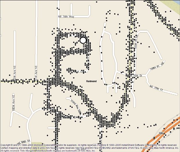
concerns were fairly light[16]. In our GPS study, only 13 of 62 (21%) whom we
asked insisted on not sharing their location data outside our institution. In 55
interviews with subjects in Finland, Kaasinen[17] found that “… the interviewees
were not worried about privacy issues with location-aware services.” However, he
adds, “It did not occur to most of the interviewees that they could be located while
using the service.”
   It may be that the implications of leaked location data will not be adequately
understood until there is a widely publicized incident of an innocent victim being
seriously harmed. A recent story[8] in the New York Daily News describes how a
suspected killer was caught via cell phone tracking, but the tracked person was not
one of the “good guys”. There have been at least two incidents in the U.S. where a
man tracked an ex-wife or ex-girlfriend by secretly installing a GPS in her car[25].
   This paper takes a different approach to exposing the risks of leaked location data
by quantitatively assessing the threat using real location tracks to infer a person’s
identity. Tracks such as these can be used benevolently to assess traffic[22], train a
system about a user’s habits[26], create customized driving routes[20], help predict
where a user is going[19], or create a travelogue[10]. To protect this data from
malicious inferences, researchers have proposed pseudonymity[27], which attaches a
persistent ID to the GPS data but that does not link the ID to the identity of the user.
Pseudonymity was the same scheme used to protect the identities of AOL search users
when their search query logs were released and subsequently retracted by AOL. The
identity of searcher pseudonym “4417749” was uncovered from the search logs by a
reporter[3]. In this paper, we assess the effectiveness of pseudonymity on GPS logs.
   Based on two-week (or longer) GPS tracks from 172 known individuals, we
developed four heuristic algorithms to identify the latitude and longitude of their
homes. From these locations, we used a free Web service to do a reverse “white
pages” lookup, which takes a latitude and longitude coordinate as input and gives an
address and name. We report the fraction of the individuals we were able to correctly
identify and the fraction whose home address we found based on our four home-
finding algorithms. We go on to assess the effectiveness of three obscuration
algorithms that attempt to alter the GPS data in a way to prevent our privacy attacks.
This is the first paper we know of to assess quantitatively the risk of identifying the
persons associated with leaked, pseudonymized location tracks.
   Analyzing data in order to illegitimately gain knowledge about a subject is known
as an “inference attack”. Our tests are intended to mimic what an attacker would do
with a large volume of location data from several individuals, assuming he or she has
defeated any encryption or access control on the data. We assume the attacker’s goal
is to identify the subjects after which he or she would nefariously profit from a
multitude of associated identities and location tracks. The large volume of data
necessitates an automated approach of the type we implement. Clearly an attacker
with a smaller set of potential victims could afford more time-consuming means of
identifying them by physically staking out their neighborhood or manually inspecting
their location tracks. Our attacks are limited to computation.
   Our tests are based on GPS data gathered from volunteer drivers, which we
describe in the next section.
2 Multiperson Location Survey

Our Microsoft Multiperson Location Survey (MSMLS) is an ongoing survey of where
people drive. We loan subjects a Garmin Geko 201 GPS receiver, capable of
automatically recording 10,000 time-stamped latitude and longitude coordinates. The
GPSs are powered from the car’s cigarette lighter, and a simple hardware
modification ensures that the GPS turns on whenever it detects available power. This
is necessary for the cars whose cigarette lighter is powered only when the car is on.
Subjects are instructed to leave the GPS on their car’s dashboard. We set up the GPS
in an adaptive recording mode so it ceases to record when the car is stopped. This
prevents the memory from filling up while the car is parked. With this recording
mode, we found that the median separation between points is 64.4 meters in distance
and 6 seconds in time. Each subject recorded data for at least two weeks.
   We recruited subjects from our institution and allowed their adult family members
to participate as well. Subjects are compensated by being entered in a drawing from
100 subjects to win an MP3 player worth about US$ 200. Before receiving the GPS
receiver, each subject fills out an online survey, whose questions include the subject’s
name, home address, and other demographic information. The subject’s name and
home address data serve as the ground truth for assessing our privacy attacks and
countermeasures. At the time of the study, we had data from 172 drivers whose
addresses were recognizable by our reverse geocoder. These are the subjects we used
for the tests in this paper. From the demographic data, 72% were male, 75% had a
domestic partner, 37% had children, and the average age of drivers was 37.
   Other location-gathering efforts include Ashbrook & Starner’s[2] two studies of
subjects with wearable GPS recorders. One had a single subject for 4 months, and the
second had six users for 7 months. Their GPS recorders could hold 200,000 points,
compared to our 10,000. Liao et al.[21] gathered GPS data from one person for four
months and subsequently five people for one week. As of this writing, the
OpenStreetMap[15] project has 5511 GPS traces contributed by volunteers in an
effort to produce copyright-free maps.

3 Inferring Home and Identity

Given a set of time-stamped latitude and longitude coordinates, the first step in our
privacy attack is to infer the coordinates of the subject’s home. This section describes
how we first computed the location of a subject’s home and then the subject’s identity
from pseudonymous GPS data.

3.1 Related Efforts

The general problem of extracting significant places from location data has received
much attention. Marmasse and Schmandt’s comMotion[24] system designated as
significant those places where the GPS signal was lost three or more times within a
given radius, normally due to a building blocking the signal, after which the user was

prompted for a place name. Marmasse’s subsequent work[23] looked at a combination
of dwell time, breaks in time or distance, and periods of low GPS accuracy as
potentially significant locations. Ashbrook & Starner[2] clustered places where the
GPS signal was lost and asked users to name such locations. Using locations
generated from Place Lab, Kang et al. [18] used time-based clustering to identify
places that the user would likely find important. Hariharan & Toyama[11] created a
time- and location-sensitive clustering technique to hierarchically represent “stays”
and “destinations”. Liao et al.[21] used this algorithm to find a user’s frequent
destinations for higher-level machine learning about a user’s habits. Hightower et
al.’s BeaconPrint[12] algorithm finds repeatable sets of GSM and Wi-Fi base stations
where a user dwells. This is interesting in that it does not use spatial coordinates as a
location indicator, but instead sets of consistently heard radio transmitters.
Subramanya et al.[30] used a dynamic probabilistic model on inputs from GPS and
other sensors to classify the user’s motion state (e.g. stationary, walking, driving, etc.)
as well as the type of location from among indoors, outdoors, or vehicle.
   Of the work above, only Liao et al.[21] made an attempt to automatically
determine which of the important places are the subject’s home. They used machine
learning on labeled place data to achieve 100% classification accuracy in finding
locations of their five subjects’ home and work places.
   The work most closely related to ours is from Hoh et al.[13] who used a database
of week-long GPS traces from 239 drivers in the Detroit, MI, USA area. Examining a
subset of 65 drivers, their home-finding algorithm was able to find plausible home
locations of about 85%, although the authors did not know the actual locations of the
drivers’ homes. Our study is based on drivers’ self-reported home addresses, and we
also attempt to infer the drivers’ names as well as home locations.

3.2 Finding Homes in GPS Traces

Our first challenge is to find the coordinates of each subject’s home based on their
GPS data. For each subject, we have a list of time-stamped latitude and longitude
points. We tested four algorithms for picking out the location of the subject’s home,
two of which depend on segmenting the GPS data into discrete trips. Our
segmentation is simple: we sort the list of points by time and split it into candidate
trips at points which are separated by more than five minutes. We then retain only
those trip segments that meet three criteria:
    1. The trip must have at least ten measured points.
    2. The trip must be at least one kilometer long.
    3. The trip must have at least one pair of points during which the speed was at
        least 25 miles/hour. This helps eliminate walking and bicycle trips which we
        are not trying to analyze.
The first two criteria tend to eliminate noise trips that result from random data
gathered from parked vehicles. The final point in each trip segment is the trip’s
destination, which gives us a list of latitude and longitude points, one for each trip,
some of which are likely the location of the subject’s home.
    These are our four heuristic algorithms for computing the coordinates of each
subject’s home:
Last Destination – This algorithm is based on the heuristic that the last destination of the day is often a subject’s home. For each day of the survey, we found the destination closest to, but not later than, 3 a.m. We computed the median latitude and longitude of these destinations for our estimate of the home location. Weighted Median – We assume that the subject spends more time at home than at any other location. Each coordinate in the survey (not just the destinations) is weighted by the dwell time at that point, i.e. the amount of time until the next point was recorded. The weighted median latitude and longitude is taken as the home location. The weighted median can be thought of as a regular median of a set of values, but values are repeated in the set proportional to a second set of corresponding weights. Thus, if a point is recorded at 8 p.m. as the subject parks his car at home, and if and nothing else recorded until 8 a.m. when the subject leaves home, the point recorded at 8 p.m. will have a much higher weight than points recorded at more frequent intervals during travel. This method implicitly accounts for the variable recording rate of our GPS receivers and it avoids the need for segmentation into trips. Largest Cluster – This heuristic assumes that most of a subject’s coordinates will be at home. We build a dendrogram of the subject’s destinations, where the merge criterion is the distance between the cluster centroids. The dendrogram is a common, agglomerative, hierarchical, clustering technique. We stop clustering when the nearest two clusters are over 100 meters apart. The home location is taken as the centroid of the cluster with the most points. Best Time – This is the most principled (and worst performing) algorithm for finding the subject’s home. It learns a distribution over time giving the probability that the subject is home. For each measured location (not just the destinations), we reverse geocoded the latitude and longitude coordinates into a street address. Reverse geocoding takes a (latitude, longitude) and returns a street address or other symbolic representation of the location. We used the MapPoint® Web Service (MPWS) as our reverse geocoder. From our survey, we took each subject’s self-reported home address and normalized it to the same format used by MPWS. Looking at 30-minute intervals in time, we computed the frequency with which the reverse geocoded points matched the subject’s actual address. In order to compensate for the GPS’s adaptive sampling times, we resampled all the measured location traces at one-minute intervals to avoid biasing the distribution away from times when points were recorded infrequently. The relative probability of being at home vs. time of day is shown in Figure 1. As expected, people are more likely to be home at night than during the day. Applying this distribution, we compute the relative probability of being home for each measured latitude and longitude for each subject. We extract those coordinates for each subject that have the maximum relative probability and take the home location as the median of those points.
Relative Probability of Home vs. T ime of Day

                   0.02
                  0.018
                  0.016                     8 a.m.             6 p.m.
                  0.014
    Probability

                  0.012
                   0.01
                  0.008
                  0.006
                  0.004
                  0.002
                      0
                   01 0
                   02 0
                   03 0
                         0
                         0

                   06 0
                   07 0
                   08 0
                   09 0
                   10 0
                   11 0
                         0
                         0

                   14 0
                   15 0
                   16 0
                   17 0
                   18 0
                   19 0
                         0

                   21 0
                   22 0
                   23 0
                         0
                      :0
                      :0
                      :0
                      :0
                      :0
                      :0
                      :0
                      :0
                      :0
                      :0
                      :0
                      :0
                      :0
                      :0
                      :0
                      :0
                      :0
                      :0
                      :0
                      :0
                      :0
                      :0
                      :0
                      :0
                   00

                   04
                   05

                   12
                   13

                   20
                                           Tim e (24 hour clock)

 Figure 1: The relative probability of a subject being at home varies depending on
 the time of day. We used this distribution in our "Best Time" algorithm to help
 determine the location of a subject's home.
   The work most similar to ours, Hoh et al.[13], used heuristics similar to ours for
finding homes based on GPS traces. They first dropped GPS samples recorded at
speeds greater than one meter/second and then applied agglomerative clustering until
the clusters reached an average size of 100 meters. They eliminated clusters with no
recorded points between 4 p.m. and midnight as well as clusters deemed outside
residential areas by manual inspection of maps.
   Although our ultimate goal is to infer identities, we can assess the performance of
our algorithms at an intermediate step by evaluating how well they locate each
subject’s home. For this evaluation, we used MPWS to geocode the location (i.e. find
the latitude and longitude coordinates) of each subject’s home based on their reported
addresses. We then computed the errors between the geocoded locations and the
inferred locations given by our four algorithms. The best performing algorithm, in
terms of median error, was “Last Destination”, whose median error was 60.7 meters.
“Weighted Median” and “Largest Cluster” had nearly the same median errors, at 66.6
meters. “Best Time” was significantly worse with a median error of 2390.2 meters.
Figure 2 shows a histogram of home location errors from the best-performing “Last
Destination” algorithm. Based on these results, we can conclude that an attacker,
using data like ours, could computationally locate a subject’s home to within about 60
meters at least half the time.
   The “Best Time” algorithm reveals an interesting characteristic of our reverse
geocoding solution. Reverse geocoding is an integral part of our privacy attack,
because it is the link from a raw coordinate to a home address and ultimately to an
identity via a white pages lookup. In developing the probability distribution for “Best
Time”, we found only 1.2% of the measured points were reverse geocoded to the
subjects’ self-reported home addresses. This is after we resampled our data at a
constant one minute interval to compensate for our GPS’s adaptive recording mode.
This is why Figure 1 shows only relative probability (normalized to a sum of one), not
the absolute probability of a subject being at home, because the computed absolute
Home Location Errors Histogram
0.14
0.12
Frequency
0.1
0.08
0.06
0.04
0.02
0
10
30
50
70
90
0
0
0
0
0
0
0
0
0
0
e
or
11
13
15
17
19
21
23
25
27
29
M
Error (meters)
Figure 2: This is a histogram of the home location errors from the "Last
Destination" algorithm. The median error was 60.7 meters.
probabilities are clearly too small. For the purposes of “Best Time”, it is enough to
know only the relative probabilities. In evaluating our reverse geocoder, it seems
extremely unlikely that our subjects collectively spend only 1.2% of their time at
home, which makes us suspicious that our reverse geocoder was usually not giving
the correct address corresponding to the measured coordinates. This is one weak point
in the type of attacks we are examining.
3.3 From Home Coordinates to Identity
Armed with a likely coordinate of a subject’s home, the final step in our privacy
attack is to find the subject’s identity. We accomplished this with a Web-based, white
pages lookup. Windows Live™ Search has a freely downloadable API[14] that allows
no-cost, programmatic access to its search capabilities. In “phone book” mode, the
search engine can be set up to return street addresses and associated names within a
given radius of a given coordinate. There are several paid services available on the
Web which give the same information.When our search engine returned multiple
results, we took the one physically nearest the given coordinate based on the search
engine’s returned latitude and longitude fields.
3.4 Attacker Summary
Summarizing our assumptions about the attacker, we assume the following:
• The attacker has access to about two weeks of time-stamped GPS data recorded
from 172 unknown drivers. The GPS receivers are in the drivers’ vehicles, not
carried on the drivers themselves. The GPS data is recorded at a median interval
of 6 seconds and 64.4 meters.
• The GPS data points for each driver are tagged with a common pseudonym such
that all the GPS data for each driver can be easily grouped together anddistinguished from data for the other drivers.
• The attack consists of first trying to computationally identify the latitude and
longitude of each driver’s home based on the GPS data. Then these coordinates
are used to find the driver’s name using a Web search.
3.5 Results
We applied the four algorithms in Section 3.2 to each of the subjects in our study.
Each algorithm gives a single coordindate as a guess for the subject’s home location.
We submitted these locations to our search engine and manually compared the
subject’s name to the name(s) returned. Sometimes the search engine returned the
names of two people living at the same address. We counted the return as a success if
it contained at least the subject’s name. We also counted the return as a success if it
returned just the subject’s first initial and last name, e.g. “G. Washington” was
considered a valid match for “George Washington”.
Of the 172 subjects, the four inference algorithms performed as follows:
Algorithm Number Correct Out of 172 Percent Correct
Last Destination 8 4.7%
Weighted Median 9 5.2%
Largest Cluster 9 5.2%
Best Time 2 1.2%
This shows that there is a legitimate danger in releasing pseudonymized location
data to potential attackers. However, the number of successful identifications was not
high. We speculate that these low rates were caused by three main types of problems:
• Measurements
o Inaccurate GPS. GPS may not report a location near enough to a
subject’s house due to its inherent inaccuracies.
o Missing GPS. Our adaptive recording mode may not have captured
points close enough to the subject’s home, especially if a subject,
upon arriving at home, drove immediately into a parking structure
that blocks GPS.
o Inaccurate home location heuristics. As shown above, our best home
location algorithm has a median error of 60.7 meters.
• Database
o Inaccurate reverse geocoding. This is apparent from the reverse
geocoding we did for the “Best Time” algorithm, in which only 1.2%
of the measured GPS points were coded to the subject’s self-reported
home address. Reverse geocoding normally works by linearly
interpolating to a house number based on addresses at the street
intersections. The reverse geocoder is generally unaware of different
sized land lots and house number gaps.
o Outdated and/or inaccurate white pages data. We performed a white
pages search for the self-reported addresses of our subjects. As shown
in Figure 3, only 33% of the subjects’ names were found listed with
their addresses. 11% of the address listings had different names listed,possibly because the subject had moved. 43% of the addresses were
not found in the white pages.
• Subject behavior
o Parking locations distant from home locations. Some subjects may
park their cars at a distance from their actual homes. Tracking the
subjects themselves rather than their vehicles may have compromised
more identies.
o Multiunit buildings. The coordinates of a parked vehicle are not a
good clue to the exact housing unit of subject who lives in an
apartment building or condominium. Using the analysis from the
Figure 3, we found that 13% of our subjects lived in multiunit
buildings.
Figure 3 shows that, based on the white pages, 33% of the subjects could have been
found, while the remainder were masked in one way or another. Despite these
vagaries, we can say that there is a least a 5% chance that an attacker can infer a
subject’s identity based on two weeks of GPS data like ours using a fairly simple
algorithm and free, Web-based lookups.
Clearly there are countermeasures available, such as encryption and strict privacy
policies. Our study is intended to highlight the need for such countermeasures by
showing how vulnerable location data is to simple privacy attacks. In the next section
White Pages Search for Name at Address
Different Name at
Address
11%
Successfully Found
Multiunit Building 33%
13%
Address Not Found
43%
Figure 3: We used our white pages search to look up the name(s) associated with
our subjects' self-reported addresses. Of all the addresses, only 33% yielded a set
of names that included the corresponding subject. The rest were either addresses in
a multiunit building giving several possible names (for which the subject usually
did not appear), a different name given for the address, or the address was not
found.we test some computational countermeasures that are designed to obscure the location
of the subject’s home by corrupting the data.
4 Countermeasures
Pseudonymity is one countermeasure to protect the identity of people if their location
history is exposed. In this section, we test three additional countermeasures that have
been previously proposed in the research literature. These could be applied to
pseudonymized location data to foil the attack presented in the previous section. In
addition to regulatory and privacy policy methods, Duckham and Kulik[7] describe a
variety of computational approaches to protecting location privacy:
Pseudonymity – This is the technique we examined above, which consists of
stripping names from location data and replacing them with arbitrary IDs.
Spatial Cloaking – Gruteser and Grunwald[9] introduce the concept of spatial
cloaking. A subject is k-anonymous if her reported location is imprecise enough for
her to be indistinguishable from at least k-1 other subjects. Scott et al. [29] speculate
that software agents could be used to implement spatial cloaking. Beresford and
Stajano[4] introduce a related concept called “mix zones”. These are physical regions
in which subjects’ pseudonyms can be shuffled among themselves to confuse an
inference attack.
Noise – If location data is noisy, it will not be useful for inferring the actual location
of the subject. This technique is called “value distortion” in Agrawal and Srikant’s
work on privacy-preserving data mining[1].
Rounding – If the location data is too coarse, it will not correspond to the subject’s
actual location. This is called “value-class membership” in [1].
Vagueness – Subjects may report a place name (e.g. home, work, school, mall)
instead of latitude and longitude. In their study on disclosure of location to social
relations, Consolvo et al.[5] found that vagueness was not popular for mobile users
communicating their locations to family and friends, although it would likely be more
acceptable for disclosure to strangers.
In addition, Hoh et al.[13] describe one other computational technique:
Dropped Samples – Hoh et al. found that reducing the GPS sampling interval from
one minute to four minutes reduced the home identification rate from 85% to 40%.
We have already tested the effectiveness of pseudonymity in the previous section.
In this section, we measure the effectiveness of noise, rounding, and one type of
spatial cloaking applied on top of pseudonymity.
These computational countermeasures contrast with information-preservingactual
home
location random
point in
small circle
r
R
data inside
large circle
deleted
Figure 4: We delete data inside the large circle to help conceal the home's location.
countermeasures like encryption and access control, which are beyond the scope of
this paper. While these other techniques may be better, we speculate that drivers
would be more comfortable releasing corrupted data than they would accepting an
authority’s promise to be careful with the uncorrupted data.
4.1 Countermeasure Specifics
Our three countermeasures apply to the raw latitude and longitude data. In a real
setting, they would be applied to the data near the source before it is transmitted
anywhere an attacker could access it. The specifics of the three methods are:
Spatial Cloaking – Previously described spatial cloaking is applied to groups of
people in the same region. We implemented an alternative that uses only a single
user’s data. It simply deletes coordinates near the subject’s home, creating ambiguity
about the home’s actual location. A simple version of the algorithm would delete all
points in a circle centered at the subject’s home. However, a geometrically-minded
attacker might be able to guess the circle’s radius and find the center. Instead, we
center the “invisibility circle” at a random point inside a smaller circle which is
centered on the home’s location. Specifically, we have a circle of radius r centered
on the home. We pick a uniformly distributed, random latitude and longitude
coordinate inside this circle as the center of a larger circle of radius R , r < R . We
delete all the measured coordinates inside the larger circle. This is illustrated in Figure
4. This process is applied to each subject with a different random point for each one.
This ensures that points at and near the home will be deleted, and the randomness for
each subject makes it more difficult for the attacker to infer the geometry of the
deletions.
Noise – We implement noise by simply adding 2D, Gaussian noise to each measuredlatitude and longitude coordinate. For each point, we generate a noise vector with a
random uniform direction over [0,2π ) and a Gaussian-distributed magnitude from
( )
N 0, σ 2 . A negative magnitude reverses the direction of the noise vector.
Rounding – We snap each latitude and longitude to the nearest point on a square grid
with spacing ∆ in meters.
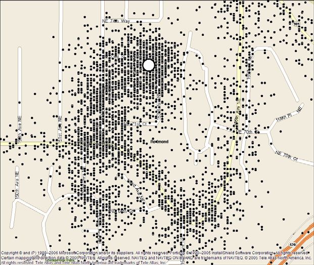
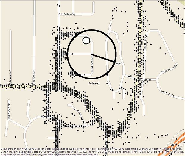
Figure 5 shows the effect of these three methods on data from one of our survey’s
subjects.
Uncorrupted GPS data Spatial Cloaking – Points inside circle
deleted. 100 meter radius circle was
centered at a random point near the
home.
Noise – Added Gaussian noise with 50 Rounding – Each point snapped to
meter standard deviation nearest point on 50 meter × 50 meter
grid.
Figure 5: This demonstrates the effect of our three methods of corrupting GPS data
to enhance privacy on a set of data from one of our subjects. The upper left image
shows the raw, uncorrupted GPS data. The white circle in each image shows the
location of the subject's house.4.2 Countermeasure Results
We evaluated the effectiveness of our three countermeasures as a function of their
various parameters. In evaluating pseudonymity above, we considered what fraction
of names we could correctly identify. However, this is highly dependent on the
quality of our white pages lookup, which we demonstrated as poor. For evaluating the
three countermeasures, we instead measured how many correct home addresses we
could find, which eliminates the uncertainty caused by poor white pages. To find the
address associated with the inferred coordinates of a home, we used the MapPoint®
Web Service. As a baseline, when run on unaltered coordinate data, the four inference
algorithms correctly find these fractions of the subjects’ home addresses:
Algorithm Number Correct Out of 172 Percent Correct
Last Destination 22 12.8%
Weighted Median 20 11.6%
Largest Cluster 19 11.0%
Best Time 6 3.5%
We are trying to find how much we have to corrupt the GPS data for the three
countermeasures to significantly reduce the number of correct address inferences.
Spatial Cloaking – To simplify presentation, we present only the best-performing
“Last Destination” algorithm for spatial cloaking. The results for varying values of R
and r (see Figure 4) are shown in Figure 6. It is not until a deletion radius R of 2000
meters that the inference rate for home addresses dropped to zero. Changing the size
Spatial Cloaking Effects
25
20
15
Number of
Correct
10 Inferences
5
0
0
10 0
0
5
15 0
50
r (meters)
0
0
10
0
0
15
0
25
25
0
0
50
50
0
10 0
75
00
75
R (meters)
00
00
10
20
Figure 6: Based on 172 subjects, spatial cloaking was not 100% effective until all
data within 2000 meters of the home was deleted.Noise Effects
25
Number of Correct
20 Last Destination
Weighted Median
Inferences
15 Largest Cluster
Best Time
10
5
0
0 50 100 150 250 500 750 1000 2000 5000
Noise Level (standard deviation in meters)
Figure 7: Adding noise with a standard deviation of five kilometers reduced the
effect of inference attacks to near zero.
of the smaller circle, radius r , did not have a noticeable effect.
Noise – The number of correct address inferences as a function of σ is shown in
Figure 7. As expected, the number of correct addresses found decreases with
increasing noise, although the amount of noise required for a significant reduction in
performance is perhaps surprising. Noise with a standard deviation of 5 kilometers
reduced the number of found addresses to only one out of 172 for three of the
inference algorithms and to zero for “Largest Cluster”.
Rounding – Coarser discretization reduced the number of correct address inferences,
which dropped to zero for all algorithms with a ∆ of 5 kilometers, as shown in Figure
8.
None of the home-finding algorithms stood out as uniquely robust at resisting the
countermeasures. Likewise, none of the countermeasures proved uniquely effective at
resisting a privacy attack. The exact points at which the countermeasures become
effective (e.g. noise level, spatial coarseness) likely do not generalize well to other
types of location data due to variations in the time between measurements, distance
between measurements, the sensor’s intrinsic accuracy and precision, and the density
of homes. From a qualitative perspective, however, the level of corruption required to
completely defeat the best inference algorithms is somewhat high.
In choosing a countermeasure, it would be important to assess not only its
effectiveness but the effect on the intended application. For instance, a traffic-
monitoring application may be relatively unaffected by cloaking a few hundred
meters around drivers’ homes, because the application uses only aggregate statistics
from multiple drivers, and because road speeds in residential neighborhoods are
relatively unimportant. On the other hand, noise or rounding could easily overpower
the map matching techniques that the traffic application would use to match GPSRounding Effects
25
20 Last Destination
Number of Correct
Weighted Median
Inferences
15 Largest Cluster
Best Time
10
5
0
0 50 100 150 250 500 750 1000 2000 5000
Discretization Delta (meters)
Figure 8: Discretizing latitude and longitude to a five-kilometer grid was enough
to protect all addresses from our inference attacks.
points to actual roads. Similar arguments apply to the applications of making
customized driving routes or travelogues, because cloaking the home location would
have only a minor effect compared to noise or rounding.
One unanswered question is the point at which a countermeasure becomes
practically effective. Even if a few addresses or identities can be compromised, the
attacker may not have any way to determine which inferences are correct. However,
more sophisticated attacks could estimate their own uncertainty, highlighting which
inferences are most likely correct.
5 Summary
This is the first paper we know of to make a thorough, experimental assessment of
computational inference attacks on recorded location data, as well as the effectiveness
of certain countermeasures. We showed that it is possible, using simple algorithms
and a free Web service, to identify people based on their pseudonymous location
tracks. Using GPS data from 172 subjects, we can find each person’s home location
with a median error of about 60 meters. Submitting these locations to a reverse white
pages lookup, we were able to correctly identify about 5% by name. This number is
low partly due to our inaccuracy in finding the home locations, but also due to the
vagaries of Web-based white pages. If we tried to identify only the home addresses,
our accuracy rose to almost 13% using a commercially available reverse geocoder.
Both the white pages and the reverse geocoder proved to be weak links in the
inference attack, but both these technologies will improve as their benevolent
applications become more important.
We tested three different countermeasures: spatial cloaking, noise, and rounding.
We quantified their effectiveness by how well they prevented our inferencealgorithms from finding the subjects’ home addresses. Our results show how much
the location data needs to be corrupted to preserve privacy. The best of our home-
finding algorithms proved somewhat robust to these techniques. The high degree of
corruption required when using noise or rounding means that several location-based
services could become unusable.
Future work on this problem should expand the experimental matrix with
additional attack algorithms and countermeasures. It would be useful to create a
quantitative assessment of the effect of the countermeasures on benevolent
applications as well as on the attack algorithms as a guide to privacy policymakers.
References
1. Agrawal, R. and R. Srikant. Privacy-Preserving Data Mining. in ACM
SIGMOD Conference on Management of Data. 2000. Dallas, TX, USA:
ACM Press.
2. Ashbrook, D. and T. Starner, Using GPS to Learn Significant Locations and
Predict Movement across Multiple Users. Personal and Ubiquitous
Computing, 2003. 7(5): p. 275-286.
3. Barbaro, M. and T.Z. Jr., A Face Is Exposed for AOL Searcher No. 4417749,
in New York Times. 2006: New York, NY USA.
4. Beresford, A.R. and F. Stajano, Location Privacy in Pervasive Computing, in
IEEE Pervasive Computing. 2003. p. 46-55.
5. Consolvo, S., et al. Location Disclosure to Social Relations: Why, When, &
What People Want to Share. in CHI '05: Proceedings of the SIGCHI
Conference on Human factors in Computing Systems. 2005. New York, NY.
6. Danezis, G., S. Lewis, and R. Anderson. How Much is Location Privacy
Worth? in Fourth Workshop on the Economics of Information Security.
2005. Harvard University.
7. Duckham, M. and L. Kulik, Location Privacy and Location-Aware
Computing, in Dynamic & Mobile GIS: Investigating Change in Space and
Time, J. Drummond, et al., Editors. 2006, CRC Press: Boca Raton, FL.
8. Gendar, A. and A. Lisberg, How Cell Phone Helped Cops Nail Key Murder
Suspect, in Daily News. 2006: New York.
9. Gruteser, M. and D. Grunwald. Anonymous Usage of Location-Based
Services through Spatial and Temporal Cloaking. in of First ACM/USENIX
International Conference on Mobile Systems, Applications, and Services
(MobiSys 2003). 2003. San Francisco, CA USA.
10. Hariharan, R., J. Krumm, and E. Horvitz. Web-Enhanced GPS. in First
International Workshop on Location- and Context-Awareness (LoCA 2005).
2005. Oberpfaffenhofen, Germany: Springer.
11. Hariharan, R. and K. Toyama. Project Lachesis: Parsing and Modeling
Location Histories. in Third International Conference on GIScience. 2004.
Adelphi, MD.
12. Hightower, J., et al. Learning and Recognizing the Places We Go. in
UbiComp 2005: Ubiquitous Computing. 2005.13. Hoh, B., et al., Enhancing Security and Privacy in Traffic-Monitoring
Systems, in IEEE Pervasive Computing. 2006. p. 38-46.
14. http://www.microsoft.com/downloads/details.aspx?FamilyId=C271309B-
02DE-42A7-B23E-E19F68667197&displaylang=en.
15. http://www.openstreetmap.org/.
16. Iachello, G., et al. Control, Deception, and Communication: Evaluating the
Deployment of a Location-Enhanced Messaging Service. in UbiComp 2005:
Ubiquitous Computing. 2005. Tokyo, Japan.
17. Kaasinen, E., User Needs for Location-Aware Mobile Services. Personal and
Ubiquitous Computing, 2003. 7(1): p. 70-79.
18. Kang, J.H., et al. Extracting Places from Traces of Locations. in 2nd ACM
International Workshop on Wireless Mobile Applications and Services on
WLAN Hotspots (WMASH'04),. 2004.
19. Krumm, J. and E. Horvitz. Predestination:Inferring Destinations from
Partial Trajectories. in Eighth International Conference on Ubiquitous
Computing (UbiComp 2006). 2006. Orange County, CA USA.
20. Letchner, J., J. Krumm, and E. Horvitz. Trip Router with Individualized
Preferences (TRIP): Incorporating Personalization into Route Planning. in
Eighteenth Conference on Innovative Applications of Artificial Intelligence
(IAAI-06). 2006. Cambridge, MA USA.
21. Liao, L., D. Fox, and H.A. Kautz. Location-Based Activity Recognition using
Relational Markov Networks. in Nineteenth International Joint Conference
on Artificial Intelligence (IJCAI 2005). 2005. Edinburgh, Scotland.
22. Lorkowski, S., et al. Towards Area-Wide Traffic Monitoring-Applications
Derived from Probe Vehicle Data. in 8th International Conference on
Applications of Advanced Technologies in Transportation Engineering.
2004. Beijing, China.
23. Marmasse, N., Providing Lightweight Telepresence in Mobile
Communication to Enhance Collaborative Living, in Program in Media Arts
and Sciences, School of Architecture and Planning. 2004, MIT: Cambridge,
MA, USA. p. 124.
24. Marmasse, N. and C. Schmandt. Location-Aware Information Delivery with
comMotion. in HUC 2K: 2nd International Symposium on Handheld and
Ubiquitous Computing. 2000. Bristol, UK: Springer.
25. Orland, K., Stalker Victims Should Check For GPS. 2003, Associated Press
on CBS News at
http://www.cbsnews.com/stories/2003/02/06/tech/main539596.shtml.
26. Patterson, D.J., et al. Opportunity Knocks: A System to Provide Cognitive
Assistance with Transportation Services. in UbiComp 2004: Ubiquitous
Computing. 2004. Nottingham, UK: Springer.
27. Pfitzmann, A. and M. Kohntopp, Anonymity, Unobservability and
Pseudonymity -- A Proposal for Terminology, in Designing Privacy
Enhancing Technologies, H. Federath, Editor. 2001, Springer-Verlag. p. 1-9.
28. Schilit, B., J. Hong, and M. Gruteser, Wireless Location Privacy Protection,
in IEEE Computer. 2003. p. 135-137.
29. Scott, D., A. Beresford, and A. Mycroft. Spatial Security Policies for Mobile
Agents in a Sentient Computing Environment. in 6th FundamentalApproaches to Software Engineering (FASE). 2003. Warsaw, Poland:
Springer-Verlag.
30. Subramanya, A., et al. Recognizing Activities and Spatial Context Using
Wearable Sensors. in 21st Conference on Uncertainty in Artificial
Intelligence (UAI06). 2006. Cambridge, MA.You can also read