Hyperspectral Super-Resolution Via Joint Regularization of Low-Rank Tensor Decomposition
←
→
Page content transcription
If your browser does not render page correctly, please read the page content below
remote sensing
Article
Hyperspectral Super-Resolution Via Joint Regularization of
Low-Rank Tensor Decomposition
Meng Cao 1 , Wenxing Bao 1,2, *                  and Kewen Qu 1,2

                                          1   School of Computer Science and Engineering, North Minzu University, Yinchuan 750021, China;
                                              20197237@stu.nun.edu.cn (M.C.); qukewen@nun.edu.cn (K.Q.)
                                          2   The Key Laboratory of Images and Graphics Intelligent Processing of State Ethnic Affairs Commission:
                                              IGIPLab, North Minzu University, Yinchuan 750021, China
                                          *   Correspondence: baowenxing@nun.edu.cn

                                          Abstract: The hyperspectral image super-resolution (HSI-SR) problem aims at reconstructing the
                                          high resolution spatial–spectral information of the scene by fusing low-resolution hyperspectral
                                          images (LR-HSI) and the corresponding high-resolution multispectral image (HR-MSI). In order to
                                          effectively preserve the spatial and spectral structure of hyperspectral images, a new joint regularized
                                          low-rank tensor decomposition method (JRLTD) is proposed for HSI-SR. This model alleviates the
                                          problem that the traditional HSI-SR method, based on tensor decomposition, fails to adequately take
                                          into account the manifold structure of high-dimensional HR-HSI and is sensitive to outliers and
                                          noise. The model first operates on the hyperspectral data using the classical Tucker decomposition to
                                          transform the hyperspectral data into the form of a three-mode dictionary multiplied by the core
                                          tensor, after which the graph regularization and unidirectional total variational (TV) regularization
                                are introduced to constrain the three-mode dictionary. In addition, we impose the l1 -norm on core

                                          tensor to characterize the sparsity. While effectively preserving the spatial and spectral structures in
Citation: Cao, M.; Bao, W.; Qu, K.        the fused hyperspectral images, the presence of anomalous noise values in the images is reduced. In
Hyperspectral Super-Resolution Via        this paper, the hyperspectral image super-resolution problem is transformed into a joint regularization
Joint Regularization of Low-Rank          optimization problem based on tensor decomposition and solved by a hybrid framework between
Tensor Decomposition. Remote Sens.        the alternating direction multiplier method (ADMM) and the proximal alternate optimization (PAO)
2021, 13, 4116. https://doi.org/
                                          algorithm. Experimental results conducted on two benchmark datasets and one real dataset show that
10.3390/rs13204116
                                          JRLTD shows superior performance over state-of-the-art hyperspectral super-resolution algorithms.

Academic Editors: Mi Wang, Hanwen
                                          Keywords: hyperspectral image super-resolution; fusion; tucker decomposition; joint regularization
Yu, Jianlai Chen and Ying Zhu

Received: 10 September 2021
Accepted: 6 October 2021
Published: 14 October 2021
                                          1. Introduction
                                                Hyperspectral images are obtained through hyperspectral sensors mounted on dif-
Publisher’s Note: MDPI stays neutral      ferent platforms, which simultaneously image the target area in tens or even hundreds
with regard to jurisdictional claims in   of consecutive and relatively narrow wavelength bands in multiple regions of the elec-
published maps and institutional affil-   tromagnetic spectrum, such as the ultraviolet, visible, near-infrared and infrared, so it
iations.                                  obtains rich spectral information along with surface image information. In other words,
                                          hyperspectral imagery combines image information and spectral information of the target
                                          area in one. The image information reflects the external characteristics such as size and
                                          shape of the sample, while the spectral information reflects the physical structure and
Copyright: © 2021 by the authors.         chemical differences within the sample. In the field of hyperspectral image processing and
Licensee MDPI, Basel, Switzerland.        applications, fusion [1] is an important element. Furthermore, the problem of hyperspectral
This article is an open access article    image super-resolution (HSI-SR) is to fuse the hyperspectral image (LR-HSI) with rich
distributed under the terms and           spectral information and poor spatial resolution with a multispectral image (HR-MSI) with
conditions of the Creative Commons        less spectral information but higher spatial resolution to obtain a high-resolution hyper-
Attribution (CC BY) license (https://     spectral image (HR-HSI). It can usually be divided into two categories: hyper-sharpening
creativecommons.org/licenses/by/          and MSI-HSI fusion.
4.0/).

Remote Sens. 2021, 13, 4116. https://doi.org/10.3390/rs13204116                                       https://www.mdpi.com/journal/remotesensing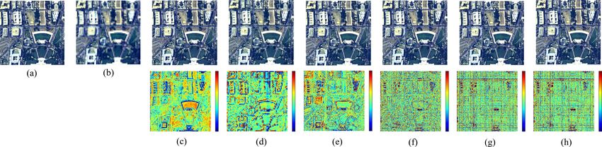
Remote Sens. 2021, 13, 4116                                                                                           2 of 27

                                    The earliest work on hyper-sharpening was an extension of pansharpening [2,3].
                              Pan-sharpening is a fusion method that takes a high-resolution panchromatic (HR-PAN)
                              image and a corresponding low-resolution multispectral (LR-MSI) image to create a high-
                              resolution multispectral image (HR-MSI). Meng et al. [4] first classified the existing pan-
                              sharpening methods into component replacement (CS), multi-resolution analysis (MRA),
                              and variational optimization (VO-based methods).
                                    The steps of the CS [5] based methods are to first project the MSI bands into a new
                              space based spectral transform, after which the components representing the spatial infor-
                              mation are replaced with HR-PAN images, and finally the fused images are obtained by
                              back-projection. Representative methods include principal component analysis (PCA) [6],
                              Gram Schmidit (GS) [7], etc. The multi-resolution analysis (MRA) [8] method is a widely
                              used method in pan-sharpening which is usually based on discrete wavelet transform
                              (DWT) [9]. The basic idea is to perform DWT on MS and Pan images, then retain the
                              approximate coefficients in MSI and replace the spatial detail coefficients with the approxi-
                              mate coefficients of PAN images to obtain the fused images. Representative algorithms
                              are smoothing filter-based intensity modulation (SFIM) [10], generalized Laplace pyramid
                              (GLP) [11], etc. VO-based [12] methods are an important class of pan-sharpening methods.
                              Since the main fusion processes of regularization-based methods [13–17], Bayesian-based
                              methods [18–20], model-based optimization (MBO) [21–23] methods and sparse reconstruc-
                              tion (SR) [24–26] based methods are all based on or transformed into an optimization of a
                              variational model, they can be generalized to variational optimization (VO) based methods.
                              In other words, the main process of such pan-sharpening methods is usually based on or
                              transformed into an optimization of a variational model. A comprehensive review of VO
                              methods based on the concept of super-resolution was first presented by Garzelli [27]. As
                              the availability of HS imaging systems increased, pan-sharpening was extended to HSI-SR
                              by fusing HSI with PANs, which is referred to as hyper-sharpening [28]. In addition, some
                              hyper-sharpening methods have evolved from MSI-HSI fusion methods [13,14,29]. In this
                              case, MSI consists of only a single band, so MSI can be simplified to PAN images [28], and
                              a more detailed comparison of hyper-sharpening methods can be found in [28].
                                    In recent years, several methods have been proposed to realize the hyper-sharpening pro-
                              cess of hyperspectral data, such as: linear spectral unmixing (LSU)-based techniques [30,31],
                              nonnegative matrix decomposition-based methods [29,32–37], tensor-based methods [38–41],
                              and deep learning-based methods to improve the spatial resolution of hyperspectral data
                              by using multispectral images. The LSU technique [30] is essentially a problem of de-
                              composing remote sensing data into endmembers and their corresponding abundances.
                              Song et al. [31] proposed a fast unmixing-based sharpening method, which uses uncon-
                              strained least squares algorithm to solve the endmember and abundance matrices. The
                              innovation of the method is to apply the procedure to sub-images rather than to the
                              whole data. Yokoya et al. [29] proposed a nonnegative matrix factorization (NMF)-based
                              hyper-sharpening algorithm called coupled NMF (CNMF) by alternately unmixing low-
                              resolution HS data and high-resolution MS data. In CNMF, the endmember matrix and
                              the abundance matrix are estimated using the alternating spectral decomposition of NMF
                              under the constraints of the observation model. However, the results of CNMF may not
                              always be satisfactory; firstly, the solution of NMF is usually non-unique, and secondly,
                              its solution process is very time-consuming because it needs to continuously alternate the
                              application of NMF unmixing to low spatial resolution hyperspectral and high spatial
                              resolution multispectral data, which yields a hyperspectral endmember and a high spatial
                              resolution abundance matrix. Later, by combining these two matrices, fused data with high
                              spatial and spectral resolution can be obtained. An HSI-SR method based on the sparse
                              matrix decomposition technique was proposed in [33], which decomposes the HSI into a
                              basis matrix and a sparse coefficient matrix. Then the HR-HSI was reconstructed using the
                              spectral basis obtained from LR-HSI and the sparse coefficient matrix estimated by HR-MSI.
                              Other NMF-based sharpening algorithms include spectral constraint NMF [34], sparse
                              constraint NMF [35], joint-criterion NMF-based (JNMF) hyper-sharpening algorithm [36],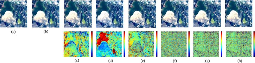
Remote Sens. 2021, 13, 4116                                                                                           3 of 27

                              etc. Specifically, some of the NMF-based methods can also be applied to the fusion process
                              of HS and PAN images, e.g., [34,35]. Furthermore, in order to obtain better fusion results,
                              the work of [37] exploited both the sparsity and non-negativity constraints of HR-HSI and
                              achieved good performance.
                                    Although many methods based on matrix decomposition under different constraints
                              have been proposed by researchers and yielded better performance, these methods based
                              on matrix decomposition require the three-dimensional remote sensing data to be expanded
                              into the form of a two-dimensional matrix, which makes it difficult for the algorithms to
                              take full advantage of the spatial spectral correlation of HSI. HSI-SR method based on tensor
                              decomposition has become a hot topic in MSI-HSI fusion research because of its excellent
                              performance. The main idea of its fusion is to treat HR-HSI as a three-dimensional tensor
                              and to redefine the HSI-SR problem as the estimation of the core tensor and dictionary in
                              three modes. Dian et al. [38] first proposed a non-local sparse tensor factorization method
                              for the HSI-SR problem (called NLSTF), which treats hyperspectral data as a tensor of three
                              modes and combines the non-local similarity prior of hyperspectral images to nonlocally
                              cluster MSI images, and although this method produced good results, LR-HSI was only
                              used for learning the spectral dictionary and not for core tensor estimation. Li et al. [39]
                              proposed the coupled sparse tensor factorization (CSTF) method, which directly decom-
                              poses the target HR-HSI using Tucker decomposition and then promotes the sparsity of
                              the core tensor using the high spatial spectral correlation in the target HR-HSI. In order to
                              effectively preserve the spatial spectral structure in LR-HSI and HR-MSI, Zhang et al. [40]
                              proposed a new low-resolution HS (LRHS) and high-resolution MS (HRMS) image fusion
                              method based on spatial–spectral-graph-regularized low-rank tensor decomposition (SS-
                              GLRTD). This method redefines the fusion problem as a low-rank tensor decomposition
                              model by considering LR-HSI as the sum of HR-HSI and sparse difference images. Then,
                              the spatial spectral low-rank features of HR-HSI images were explored using the Tucker
                              decomposition method. Finally, the HR-MSI and LR-HSI images were used to construct
                              spatial and spectral graphs, and regularization constraints were applied to the low-rank
                              tensor decomposition model. Xu et al. [41] proposed a new HSI-SR method based on a
                              unidirectional total variational (TV) approach. The method has decomposed the target
                              HR-HSI into a sparse core tensor multiplied by a three-mode dictionary matrix using
                              Tucker decomposition, and then applied the l1 -norm to the core tensor to represent the
                              sparsity of the target HR-HSI and the unidirectional TV three dictionaries to characterize
                              the piecewise smoothness of the target HR-HSI. In addition, tensor ring-based super-
                              resolution algorithms for hyperspectral images have recently attracted the attention of
                              research scholars. He et al. [42,43] proposed a HSI-SR method based on a constrained tensor
                              ring model, which decomposes the higher-order tensor into a series of three-dimensional
                              tensors. Xu et al. [44] proposed a super-resolution fusion of LR-HSI and HR-MSI using a
                              higher-order tensor ring method, which preserves the spectral information and core tensor
                              in a tensor ring to reconstruct high-resolution hyperspectral images.
                                    Deep learning has received increasing attention in the field of HSI-SR with its superior
                              learning performance and high speed. However, deep learning-based methods usually
                              require a large number of samples to train the neural network to obtain the parameters of
                              the network.
                                    The Tucker tensor decomposition is a valid multilinear representation for high-
                              dimensional tensor data, but it fails to take the manifold structures of high-dimensional
                              HR-HSI into account. Furthermore, the graph regularization can perfectly preserve local
                              information of high-dimensional data and achieve good performances in many fusion tasks.
                              Moreover, the existing tensor decomposition-based methods are sensitive to outliers and
                              noise, there is still much room for improvement. We propose a new method based on joint
                              regularization low-rank tensor decomposition (JRLTD) in this paper to solve the HSI-SR
                              problem from the tensor perspective. The model operates on hyperspectral data using the
                              classical Tucker decomposition and introduces graph regularization and the unidirectional
                              total variation regularization (TV), which effectively preserves the spatial and spectral
Remote Sens. 2021, 13, 4116 4 of 27
structures in the fused hyperspectral images while reducing the presence of anomalous
noise values in the images, thus solving the HSI-SR problem. The main contributions of
the paper are summarized as follows.
(1) In the process of recovering high-resolution hyperspectral images (HR-HSI), joint
regularization is considered to operate on the three-mode dictionary. The graph
regularization can make full use of the manifold structure in LR-HSI and HR-MSI,
while the unidirectional total variational regularization fully considers the segmen-
tal smoothness of the target image, and the combination of the two can effectively
preserve the spatial structure information and the spectral structure information of
HR-HSI.
(2) Based on the unidirectional total variational regularization, the l2,1 -norm is used. The
l2,1 -norm is not only sparse for the sum of the absolute values of the matrix elements,
but also requires row sparsity.
(3) During the experiments, not only the standard dataset of hyperspectral fusion is
adopted, but also the dataset about the local Ningxia is used, which makes the
algorithm more widely suitable and the performance more convincing.
The remainder of this paper is organized as follows. Section 2 presents theoretical
model and related work. Section 3 describes the solution to the optimization model.
Section 4 describes our experimental results and evaluates the algorithm. Conclusions and
future research directions are presented in Section 5.
2. Related Works
We introduce the definition and representation of the tensor, discuss the basic problems
of image fusion, and introduce the concept of joint regularization.
2.1. Tensor Description
In this paper, the capital flower font T ∈ R I1 × I2 ×···× IN denotes the Nth order tensor,
and each element in the tensor can be obtained by fixing the subscript: Ti1 ,i2 ···i N ∈ R. In
addition, to distinguish the tensor representation, this paper uses the capital letter to denote
the matrix, e.g., X ∈ R I1 × I2 ; the lower case letter denotes the vector, e.g., x ∈ R I . Tensor
vectorization is the process of transforming a tensor into a vector. For example, a tensor
T ∈ R I1 × I2 ×···× IN of order N is tensorized to a vector T ∈ R I1 ∗ I2 ∗···∗ IN , which can be
expressed as τ = vec(T ). The elemental correspondence between them is as follows:
Ti1 ,i2 ···i N = τi1 + I1 ∗(i2 −1)+···+ I1 ∗ I2 ∗···∗ IN −1 ∗(id −1) (1)
An n-mode expansion matrix is defined by arranging the n-mode fibers of a tensor
as columns of a matrix, e.g., T(n) = un f old(T ) ∈ R In × I1 I2 ··· In−1 In+1 ··· IN . Conversely, the
inverse of the expansion can be defined as T = f old T(n) . The n-mode product of a
tensor T ∈ R I1 × I2 ×···× IN and a matrix P ∈ R J × In , denoted T × n P, is a tensor A of size
I1 × · · · × In−1 × J × In+1 × · · · × IN . The n-mode product can also be expressed as each
n-model fiber multiplied by a matrix, denoted A(n) = PT(n) .
For tensor data, as the dimensionality and order increase, the number of parameters
will exponentially skyrocket, which is called dimensional catastrophe or dimensional
curse, and tensor decomposition can alleviate this problem well. Commonly used tensor
decomposition methods include CP decomposition, Tucker decomposition, Tensor Train
decomposition, and tensor Ring decomposition. In this paper, the Tucker decomposition
method is mainly adopted to operate the tensor data. Tucker decomposition, also known
as a form of higher-order principal component analysis, decomposes a tensor into a core
tensor multiplied by a factor matrix along each modality, with the following equation:
T = C × 1 P1 × 2 P2 × · · · × N P N (2)Remote Sens. 2021, 13, 4116 5 of 27
where Pi ∈ R Ii ×ri denotes the factor matrix along the ith order modality. The core tensor de-
scribing the interaction of the different factor matrices can be denoted by C ∈ Rr1 ×r2 ×···×r N .
The matrixed form of the Tucker decomposition can be defined as:
T(i) = Pi C(i) ( PN ⊗ · · · ⊗ Pi+1 ⊗ Pi−1 ⊗ · · · ⊗ P1 )T (3)
where ⊗ is the Kronecker product. The l1 -norm of r
the tensor is defined as kT k1 =
2
∑ i1 ,··· ,i N τi and the F-norm is defined as kT k F = ∑ i1 ,··· ,i N τi .
1 ,··· ,i N 1 ,··· ,i N
2.2. Observation Model
The desired HR-HSI can be defined as X ∈ R NW × NH × NS , the LR-HSI can be denoted
as Y ∈ R Nw × Nh × NS (0 < Nw < NW , 0 < Nh < NH ), the HR-MSI can be defined as
Z ∈ R NW × NH × Ns (0 < Ns < NS ). The dimensions of the spatial pattern are NW and
NH , and NS denotes the dimension of the spectral mode. From the definition of tensor
decomposition, we can derive the basic form of hyperspectral high resolution, i.e.,
X = C × 1 P1 × 2 P2 × 3 P3 (4)
The LR-HSI Y can be expressed as the spatial down-sampling form of the desired
HR-HSI X, i.e.,
Y = C × 1 P̂1 × 2 P̂2 × 3 P3 (5)
The HR-MSI Z can be expressed as the spectral down-sampling form of the desired
HR-HSI X, i.e.,
Z = C × 1 P1 × 2 P2 × 3 P̂3 (6)
where C ∈ Rnw ×nh ×ns is the core tensor, S1 ∈ R Nw × NW , S2 ∈ R Nh × NH , S3 ∈ R Ns × NS are the
down-sampling matrices, and P1 ∈ R NW ×nw , P2 ∈ R NH ×nh , P3 ∈ R NS ×ns are the dictionaries
in the three modes, then, P̂1 , P̂2 , P̂3 are the down-sampling dictionaries in the three modes,
which can be derived from the following equation:
P̂1 = S1 P1 ∈ R Nw ×nw , P̂2 = S2 P2 ∈ R Nh ×nh , P̂3 = S3 P3 ∈ R Ns ×ns (7)
2.3. Joint Regularization
Based on the Tucker decomposition and the factor matrix processed along the tri-mode
downsampling, the HSI-SR problem can be expressed by the following equation:
2 2
min Y − C × 1 P̂1 × 2 P̂2 × 3 P3 F
+ Z − C × 1 P1 × 2 P2 × 3 P̂3 F
P1 ,P2 ,P3 ,C (8)
s.t.kCk0 6 N
where k·k F denotes the Frobenius norm and N denotes the number of nonzero entries in
matrix. Clearly, the optimization problem in (8) is non-convex. Aiming for a tractable and
scalable approximation optimization, we impose the l1 -norm on the core tensor instead of
the l0 -norm to formulate the unconstrained version and describe the sparsity in spatial and
spectral dimensions.
2 2
min Y − C × 1 P̂1 × 2 P̂2 × 3 P3 F
+ Z − C × 1 P1 × 2 P2 × 3 P̂3 F
+ λ1 kCk1 (9)
P1 ,P2 ,P3 ,C
Regardless, problem (9) is still a non-convex problem of discomfort. Therefore, to
solve problem (9), some prior information about the target HR-HSI is needed. In this
paper, we consider the spectral correlation and spatial coherence of hyperspectral and
multispectral images.
As we all know, HSI suffers from high correlation and redundancy in the spectral
space and retains the fundamental information in the low-dimensional subspace. BecauseRemote Sens. 2021, 13, 4116 6 of 27
of the lack of appropriate regularization item, the fusion model in (9) is sensitive to
outliers and noise. Therefore, to accurately estimate the HSI, we used a joint regularization
(graph regularization and unidirectional total variation regularization) in the form of
a constraint on the HR-MSI and LR-HSI. To obtain accurate results for the target HR-
HSI, we first assume that the spatial and spectral manifold information between HR-MSI
and LR-HSI is similar to the embedded in the target HR-HSI, and describe the manifold
information present in HR-MSI and LR-HSI in the form of two graphs: one based on the
spatial dimension and the other on the spectral dimension. Thus, the spatial and spectral
information from HR-MSI and LR-HSI can be transferred to HR-HSI by spatial and spectral
graph regularization, which can preserve the intrinsic geometric structure information
of HR-MSI and LR-HSI as much as possible. After that, we used a unidirectional total
variation regularization model to manipulate the three-mode dictionary for the purpose of
eliminating noise in the images.
2.3.1. Graph Regularization
We know that the pixels in HR-MSI do not exist independently and the correlation
between neighboring pixels is very high. Scholars generally use a block strategy to define
adjacent pixels, but this ignores the spatial structure and consistency of the image. As a
hyper segmentation method, the hyper-pixel technique not only captures image redundant
information, but also adaptively adjusts the shape and size of spatial regions. Considering
the compatibility and computational complexity of superpixels, the entropy rate superpixel
(ERS) segmentation method is employed in this paper to find spatial domains adaptively.
The construction of the spatial graph consists of four steps: generating intensity images,
superpixel segmentation, defining spatial neighborhoods, and generating spatial graphs.
In contrast, for LR-HSI, its neighboring bands are usually contiguous, meaning that the
neighboring bands have extremely strong correlation in the spectral domain. To further
maintain the correlation and consistency in HR-HSI, we leverage the nearest neighbor
strategy to establish the spectral graph.
2.3.2. Unidirectional Total Variation Regularization
Hyperspectral images are susceptible to noise, which seriously affects the image
visual quality and reduces the accuracy and robustness of subsequent algorithms for image
recognition, image classification and edge information extraction. Therefore, it is necessary
to study effective noise removal algorithms. Common algorithms have the following three
categories: the first type of methods is filtering method, including spatial domain filtering
and transform domain filtering; the second type of methods is matching method, including
moment matching method and histogram matching method; the third type of methods is
variation method.
The best known of the variation methods is the total variation (TV) model, an algo-
rithm that has proven to be one of the most effective image denoising techniques. The
total variation model is an anisotropic model that relies on gradient descent for image
smoothing, hoping to smooth the image as much as possible in the interior of the image
(with small differences between adjacent pixels), while not smoothing as much as possible
at the edges of the image. The most distinctive feature of this model is that it preserves the
edge information of the image while removing the image noise. In general, scholars impose
the l1 -norm on the total variation model to obtain better denoising effect by improving the
total variation model or combining the total variation model with other algorithms. When
l1 -norm is used in the model, it is insensitive to smaller outliers but sensitive to larger ones;
when l2 -norm is used, it is insensitive to larger outliers and sensitive to smaller ones; and
when lσ -norm is used, it can be adjusted by tuning the parameters to be between l2 -norm
and l1 -norm, so that the robustness of both l1 -norm and l2 -norm is utilized regardless of
whether the outliers are large or small, but the burden of tuning parameters σ is increased.
In order to solve the above problem, the l2,1 -norm makes the total variation model better
handle outliers and reduce the burden of tuning parameters, acting as a flexible embeddingRemote Sens. 2021, 13, 4116 7 of 27
without the burden of tuning parameters of the lσ -norm. Therefore, in this paper, we
impose the l2,1 -norm on the unidirectional total variation model to achieve the purpose of
noise removal.
2.4. Proposed Algorithm
Combining the observation model proposed in Section 2.2 with the joint regularization
constraint proposed in Section 2.3, the following fusion model is obtained to solve the
HSI-SR problem, i.e.,
2 2
min Y − C × 1 P̂1 × 2 P̂2 × 3 P3 F + Z − C × 1 P1 × 2 P2 × 3 P̂3 F + λ1 kCk1
P1 ,P2 ,P3 ,C
+ βtr P3T PS P3 + γtr ( P2 ⊗ P1 )T PD ( P2 ⊗ P1 ) (10)
+ λ2 Dy P1 2,1
+ λ3 Dy P2 2,1
+ λ4 Dy P3 2,1
s.t.X = C × 1 P1 × 2 P2 × 3 P3
where X denotes the desired HR-HSI, Y denotes the acquired LR-HSI, Z denotes the HR-
MSI of the same scene, P1 , P2 , P3 are the dictionaries in the three modes, C is the core
tensor, P̂1 , P̂2 , P̂3 are the down-sampling dictionaries in the three modes, PS , PD are the
graph Laplacian matrices, β, γ are the equilibrium parameters of the graph regularization,
λi (i = 1, 2, 3, 4) are the positive regularization parameters, Dy is a finite difference operator
along the vertical direction, given by the following equation:
1 −1 0 0 · · · 0
0 1 −1 0 · · · 0
.. .. .. .. .. ..
Dy = .
. . . . . (11)
. . . . . .
.. .. .. .. .. ..
0 0 ··· 0 1 −1
Next, we will give an effective algorithm for solving Model (10).
3. Optimization
The proposed model (10) is a non-convex problem by solving P1 , P2 , P3 and C jointly,
and we can barely obtain the closed-form solutions for P1 , P2 , P3 and C . We know that
non-convex optimization problems are considered to be very difficult to solve because the
set of feasible domains may have an infinite number of local optima; that is to say, the
solution of the problem is not unique. However, with respect to each block of variables, the
model proposed in (10) is convex while keeping the other variables fixed. In this context,
we utilize the proximal alternating optimization (PAO) scheme [45,46] to solve it, which is
ensured to converge to a stationary point under certain conditions. Concretely, the iterative
update of model (10) is as follows:
pre 2
P1 = arg min f ( P1 , P2 , P3 , C) + ρ P1 − P1
P1 F
pre 2
P2 = arg min f ( P1 , P2 , P3 , C) + ρ P2 − P2
P2 F
2
(12)
pre
C) −
P3 = arg min f ( P , P
1 2 3 , P , + ρ P3 P 3 F
P3
2
pre
C = arg min f ( P1 , P2 , P3 , C) + ρkC − C k F
C
where the objective function f ( P1 , P2 , P3 , C) is the implicit definition of (10), and (·) pre
and ρ represent the estimated blocks of variables in the previous iteration and a positive
number, respectively. Next, we present the solution of the four optimization problems in
(12) in detail.Remote Sens. 2021, 13, 4116 8 of 27
3.1. Optimization of P1
With fixing P2 , P3 and C , the optimization problem of P1 in (12) is given by
2 2 pre 2
arg min Y − C × 1 P̂1 × 2 P̂2 × 3 P3 F
+ Z − C × 1 P1 × 2 P2 × 3 P̂3 F
+ ρ P1 − P1
P1 F
(13)
T
+ γtr ( P2 ⊗ P1 ) PD ( P2 ⊗ P1 ) + λ2 Dy P1 2,1
pre
where P1 denotes the estimated dictionary of width mode in the previous iteration and
Dy ∈ R( NW −1)× NW denotes the difference matrix along the vertical direction of P1 . Using
the properties of n-mode matrix unfolding, problem (13) can be formulated as
2 2 pre 2
arg min Y(1) − S1 P1 A1 + Z(1) − P1 B1 + ρ P1 − P1
P1 F F F
(14)
T
+ γtr ( P2 ⊗ P1 ) PD ( P2 ⊗ P1 ) + λ2 Dy P1 2,1
where Y(1) and Z(1) are the width-mode (1-mode) unfolding matrix of tensors Y and Z,
respectively, A1 = C × 2 P̂2 × 3 P3 (1) , and B1 = C × 2 P2 × 3 P̂3 (1) .
3.2. Optimization of P2
With fixing P1 , P3 and C , the optimization problem of P2 in (12) is given by
2 2 pre 2
arg min Y − C × 1 P̂1 × 2 P̂2 × 3 P3 F
+ Z − C × 1 P1 × 2 P2 × 3 P̂3 F
+ ρ P2 − P2
P2 F
(15)
T
+ γtr ( P2 ⊗ P1 ) PD ( P2 ⊗ P1 ) + λ3 Dy P2 2,1
pre
where P2 denotes the estimated dictionary of height mode in the previous iteration and
Dy ∈ R( NH −1)× NH denotes the difference matrix along the vertical direction of P2 . Using
the properties of n-mode matrix unfolding, problem (15) can be formulated as
2 2 pre 2
arg min Y(2) − S2 P2 A2 + Z(2) − P2 B2 + ρ P2 − P2
P2 F F F
(16)
T
+ γtr ( P2 ⊗ P1 ) PD ( P2 ⊗ P1 ) + λ3 Dy P2 2,1
where Y(2) and Z(2) are the height-mode (2-mode) unfolding matrix of tensors Y and Z,
respectively, A2 = C × 1 P̂1 × 3 P3 (2) , and B2 = C × 1 P1 × 3 P̂3 (2) .
3.3. Optimization of P3
With fixing P1 , P2 and C , the optimization problem of P3 in (12) is given by
2 2 pre 2
arg min Y − C × 1 P̂1 × 2 P̂2 × 3 P3 F
+ Z − C × 1 P1 × 2 P2 × 3 P̂3 F
+ ρ P3 − P3
P3 F
(17)
+ βtr P3T PS P3 + λ4 Dy P3 2,1
pre
where P3 denotes the estimated spectral dictionary in the previous iteration and Dy ∈
R( NS −1)× NS denotes the difference matrix along the vertical direction of P3 . Using the
properties of n-mode matrix unfolding, problem (17) can be formulated as
2 2 pre 2
arg min Y(3) − P3 A3 + Z(3) − S3 P3 B3 + ρ P1 − P1
P3 F F F
(18)
+ βtr P3T PS P3 + λ4 Dy P3 2,1Remote Sens. 2021, 13, 4116 9 of 27
where Y(3) and Z(3) are the spectral-mode (3-mode) unfolding matrix of tensors Y and Z,
respectively, A3 = C × 1 P̂1 × 2 P̂2 (3) , and B3 = C × 1 P1 × 2 P2 (3) .
3.4. Optimization of C
With fixing P1 , P2 and P3 , the optimization problem of C in (12) is given by
2 2
arg min Y − C × 1 P̂1 × 2 P̂2 × 3 P3 F
+ Z − C × 1 P1 × 2 P2 × 3 P̂3 F
C (19)
+ λ1 kCk1 + ρkC − C pre k2F
where C pre represents the estimated core tensor in the previous iteration.
It should be noted that problems (14), (16), (18) and (19) are convex problems. There-
fore, all these four subproblems can be effectively solved using fast and accurate ADMM
technique. Due to the similarity of the solution process of problems (14), (16), and (18), we
include the solution details of the four subproblems and the optimization updates of each
variable as appendices for more conciseness. In Appendix A, Algorithms A1–A4 draw a
summary of the solution process of the four subproblems in (12).
Algorithm 1 specifies the steps of the JRLTD-based hyperspectral image super-resolution
proposed in this section.
Algorithm 1 JRLTD-Based Hyperspectral Image Super-Resolution.
1: Initialize P1 , P2 through the DUC-KSVD algorithm [47];
2: Initialize P3 through the SISAL algorithm [48];
3: Initialize C through the Algorithm A4;
4: while not converged do
5: Step 1 Update the width mode dictionary matrix P1 via Algorithm A1;
pre
6: P̂1 = S1 P1 , P1 = P1 ;
7: Step 2 Update the height mode dictionary matrix P2 via Algorithm A2;
pre
8: P̂2 = S2 P2 , P2 = P2 ;
9: Step 3 Update the spectral dictionary matrix P3 via Algorithm A3;
pre
10: P̂3 = S3 P3 , P3 = P3 ;
11: Step 4 Update the core tensor C via Algorithm A4;
12: C pre = C ;
13: end while
14: Estimating target HR-HSI X via formula (4)
4. Experiments
4.1. Datasets
In this section, three datasets are used to test the performance of the proposed method.
The first dataset is the Pavia University dataset, which was acquired by the Italian
Reflection Optical System Imaging Spectrometer (ROSIS) optical sensor in the downtown
area of the University of Pavia. The image size is 610 × 340 × 115, with a spatial resolution
of 1.3 m. We reduced the number of spectral bands to 93 after removing the water vapor
absorption band. For reasons related to the down-sampling process, only the 256 × 256 × 93
image in the upper left corner was used as a reference image in the experiment.
The second dataset is the Washington DC dataset, which is obtained from the Washing-
ton shopping mall acquired by the HYDICE sensor, intercepting images of size 1280 × 307
for annotation. The spatial resolution is 2.5m and contains a total of 210 bands. We intercept
a part of the image with the size of 256 × 256 × 191 for the experiment and use it as a
reference image.
The third dataset is the Sand Lake in Ningxia of China, which is a scene acquired
from the GF-5 AHSI sensor during the flight activity in Ningxia. The original image size
is 2774 × 2554 × 330, its spatial resolution is 30 m, and the image has 330 bands, and theRemote Sens. 2021, 13, 4116 10 of 27
experiments reduce the spectral bands to 93 to obtain the reference image size of Sand Lake
as 256 × 256 × 93.
4.2. Compared Algorithms
We selected classical and currently popular fusion methods for comparison, including
CNMF [29], HySure [18], NLSTF [38], CSTF [39], and UTV-HSISR [41]. The experiment
was run on a PC equipped with an Intel Core i5-9300HF CPU, 16 GB RAM and NVIDIA
GTX 1660Ti GPU. The Windows 10 x64 operating system was used and the programming
application was Matlab R2016a.
4.3. Quantitative Metrics
For the evaluation of image fusion, it is more important to obtain more convincing val-
ues from objective metrics in addition to observing the results from subjective assumptions.
To evaluate the fusion output in the numerical results, we use the following eight metrics,
namely the peak signal-to-noise ratio (PSNR), which is an objective measure of image
distortion or noise level; the error relative global dimensionless synthesis (ERGAS) to
measure the comprehensive quality of the fused results; the spectral angle mapping (SAM)
represents the absolute value of the spectral angle between two images; the root mean
square error (RMSE) is used to measure the deviation between the predicted value and
true value; the correlation coefficient (CC), which indicates the ability of the fused image
to retain spectral information; the degree of distortion (DD), which is used to indicate the
degree of distortion between the fused image and the ground truth image; the structural
similarity (SSIM) and the universal image quality index (UIQI), which measures the degree
of structural similarity between the two images.
The concept of mean squared deviation is first defined in the paper:
NW −1 NH −1
1
MSE =
NW NH ∑ ∑ [ I (i, j) − J (i, j)]2 (20)
i =0 j =0
where NW and NH denote the size of the image, I denotes a noise-free image, and J denotes
a noisy image. Then PSNR is defined as:
!
MAXi2
PSNR = 10 · log10 (21)
MSE
where MAX denotes the maximum number of pixels of the image. After that, the metrics
we use to evaluate the fused image can be expressed by the following equation:
1
PSNR X, X̃ = PSNR Xi , X̃i (22)
NS
v
1 NS MSE X, X̃
u
100 u
NS i∑
ERGAS X, X̃ = t (23)
S =1 MEAN X̃
NW NH
1 X, X̃
∑ arc cos kX k · X̃
SAM X, X̃ = (24)
NW NH i =1 i 2 i 2
s
X, X̃ F
RMSE X, X̃ = (25)
NW NH NS
N N
∑i=W1 ∑ j=H1 [ X (i, j) − VX ] · X̃ (i, j) − VX̃
CC X, X̃ = q 2 (26)
N N 2 N N
∑i=W1 ∑ j=H1 [ X (i, j) − VX ] · ∑i=W1 ∑ j=H1 X̃ (i, j) − VX̃Remote Sens. 2021, 13, 4116 11 of 27
M 2 X̄ , ¯ +c
X̃ 2σ ¯ + c
1 i i 1 X̄ X̃ 2
∑ i i
SSI M X, X̃ =
2
(27)
M i =1
( X̄i ) + X̃¯ i + c1 σX2 + σX̃2 + c2
2
i i
1
DD X, X̃ = vec( X ) − vec X̃ 1
(28)
NW NH NS
1 M 4σ2 ¯ · X̄i , X̃¯ i
∑
X̄i X̃i
U IQI X, X̃ = 2 (29)
M
X̃¯ i
2
i =1 σ + σ 2 2
X X̃
i
+ ( X̄ i ) +
i
where NS denotes the number of bands; S denotes the spatial downsampling factor; X i ,
X̃ i denote the value ofthe ith band of the ground truth image and the fused image,
respectively; MEAN Z̃ denotes the mean value of each band image; VX denotes the
mean pixel value of the original image; VX̃ is the mean pixel value of the fused image; M
denotes the sliding window; X̄ i , X̃¯ i denotes the mean value of X, X̃, respectively; σX i , σX̃
i
denotes the standard deviation of X, X̃, respectively; c1 , c2 are constants; σX2 denotes the
i , X̃ i
covariance of X i , X̃ i . Furthermore, σX2 , σX̃2 denotes the variance of X i , X̃ i , respectively. It
i i
should be noted that the best value of ERGAS, SAM, RMSE and DD is 0, the best value of
CC, SSIM and UIQI is 1, and the best value of PSNR is ∞.
4.4. Parameters Discussion
JRLTD is mainly related to the following parameters, i.e., the number of PAO iterations
K , the weights of the proximal terms ρ, the sparse regularization parameters λ1 , the smooth
regularization parameters λ2 , λ3 and λ4 , the graph regularization parameters β and γ, and
the number of three-mode dictionaries Nw , Nh and Ns .
According to the description of Algorithm 1, we use the PAO scheme to solve the
problem (10). The change of PSNR caused by the change in the number of PAO iterations
K is shown in Figure 1. In Figure 1, all three datasets show a fast increasing trend of PSNR
as K goes from 1 to 10. For the PAVIA dataset, there is a slight fluctuation in PSNR when K
varies from 10 to 50, and the maximum number of iterations of PAVIA is set to 20 in the
experiment. The Washington dataset reached the maximum PSNR when K = 25, so we set
the maximum number of iterations of the algorithm in Washington to 25. Similarly, we set
the maximum number of iterations for Sand Lake as 20.
Figure 1. PSNR values for different K.
The parameter ρ is the weight of the proximal term in (12). For the evaluation of the
influence of ρ, we perform the method for different ρ. Figure 2 presents the change of PSNR
values of the fused HSIs of the three datasets with different log ρ values (the base of log is
10). In the experiments of this paper, we take the range of log ρ to be set to [−3, 0]. As isRemote Sens. 2021, 13, 4116 12 of 27
displayed in Figure 2, there is a rise trend of PSNR for all three datasets as log ρ varies from
−3 to −1, reaches a maximum when log ρ equals −1, and decreases sharply when log ρ is
greater than −1. Therefore, we set log ρ to −1, i.e., we take ρ = 0.1 for all three datasets.
Figure 2. PSNR values for different log ρ.
The regularization parameter λ1 in (10) controls the sparsity of the core tensor, there-
fore, λ1 affects the estimation of the HR-HSI. Higher values of λ1 yield sparser core tensor.
Figure 3 shows the PSNR values of the reconstructed HSI for the Pavia University dataset
under different log λ1 . In this work, we set the range log λ1 of to [−9, −2]. As shown in
Figure 3, when log λ1 belongs to [−9, −5], the PSNR stays relatively stable; when log λ1
belongs to [−5, −4], the PSNR decreases slowly; and when log λ1 > −4, the PSNR decreases
sharply. Therefore, we set log λ1 as −6, that is, λ1 = 10−6 for the Pavia University dataset.
By the same token, the values for the Washington dataset and the Sand Lake dataset can be
decided in the same way.
Figure 3. PSNR values for different log λ1 .
The unidirectional total variation regularization parameters λ2 , λ3 and λ4 control the
segmental smoothness of the width-mode, height-mode and spectral-mode dictionaries,
respectively. Figure 4 shows the reconstructed PSNR values of HSI for the Pavia University
dataset with different log λ2 , log λ3 and log λ4 . In the experiments of this paper, we set the
range of values of log λ2 and log λ3 both to [−9, −2] and the range of values of log λ4 to
[−4, 4]. As shown in Figures 4 and 5, the PSNR reaches its peak value when log λ2 = −8,
log λ3 = −7, and log λ4 = 2. Therefore, for Pavia University dataset, we set log λ2 as −8,
log λ3 as −7, and log λ4 as 2. It is worth noting that the optimal value of λ4 is relatively large
compared of λ2 and λ3 , due to the fact that HSI is continuous in the spectral dimension,Remote Sens. 2021, 13, 4116 13 of 27
which leads to a potentially smaller full variation regularization of the dictionary along the
spectral direction. Therefore, the optimal value of its regularization parameter should be
relatively large. Similarly, the values of λ2 , λ3 and λ4 for the Washington and Sand Lake
datasets can be determined in the same way.
The graph regularization parameters β and γ control the spectral structure of the
spectral graph and the spatial correlation of the spatial graph, respectively. Figure 6 shows
the reconstructed PSNR values of HSI for the Pavia University dataset under different β
and γ. In the experiments of this paper, we take the value range of both log β and log γ to
[−7, −1]. As shown in Figure 6, the PSNR reaches its peak value when log β = −1 and
log γ = −1. Therefore, for the Pavia University dataset, we set log β as −1 and log γ as −1.
Similarly, the β and γ values for the Washington dataset and the Sand Lake dataset can be
determined in the same way.
Figure 4. PSNR values for different log λ2 and log λ3 .
Figure 5. PSNR values for different λ4 .
The number of atoms in the three-model dictionaries are nw , nh and ns . Figure 7 shows
the PSNR values of the fused HSI of the Pavia University dataset for different nw and nh ,
and Figure 8 shows the PSNR values of the fused HSI of the Pavia University dataset for
different ns . In this paper, we set the range of values for both nw and nh to [260, 400], and
set ns as [3, 21]. This is because the spectral features of HSI exist on the low-dimensional
subspace. As shown in Figure 7, the PSNR increases sharply when nw is varied in the
range [260, 360] and reaches a maximum at nw = 360, while it tends to decrease when nw
is varied in the range [360, 400]. Therefore, we set nw as 360. It should be noted that the
PSNR reaches its peak value when nh is 400, but what we have to consider is the overall
performance of other evaluation indicators, so we set nh as 380 in the paper. It can be seenRemote Sens. 2021, 13, 4116 14 of 27
from Figure 8 that the PSNR decreases with ns > 15. Therefore, we set nw = 360, nh = 400,
and ns = 15 for the Pavia University dataset. Similarly, the values of nw , nh and ns for the
Washington dataset and the Sand Lake dataset can be determined in the same way.
Figure 6. PSNR values for different log β and log γ.
Figure 7. PSNR values for different nw and nh .
Figure 8. PSNR values for different ns .
In Table 1, we give the tuning ranges for the 11 main parameters, give the values
of each parameter for the three HSI datasets mentioned in Section 4.1, and show the
recommended ranges for each parameter to easily tune the parameters.Remote Sens. 2021, 13, 4116 15 of 27
Table 1. Discussion of the main parameters.
Parameters Tuning Ranges Pavia University Dataset Washington DC Dataset Sand Lake Dataset Suggested Ranges
K [1, 50] 20 25 20 [20, 50]
−3 0 10−1 10−1 10−1 −1 0
ρ 10−9 , 10−1 10−7 , 10−6
λ1 10 ,
−9 −2 10 10−6 10−6 10−7 10 , 10
10−8 10−7 10−8
−8 −7
λ2 10−9 , 10−2 10−6 , 10−5
λ3 10 −4, 10 4 10−6 10−6 10−5 10
1 , 102
λ4 10−7 , 10−1 102 102 101 10 , 10
β 10−7 , 10−1 10−1 10−1 10−3 −3 −1
10−2 , 10−1
γ 10 , 10 10−1 10−2 10−1 10 , 10
Nw [260, 400] 360 340 360 [340, 360]
Nh [260, 400] 380 380 380 [380, 400]
Ns [3, 21] 15 15 18 [15, 18]
4.5. Experimental Results
In this section, we show the fusion results of the five tested methods for the Pavia
University, Washington DC, and Sand Lake datasets.
4.5.1. Experiment On Pavia University
In order to better display more spatial detail information and fusion results, we select
three bands (R:61, G:25, B:13) to be synthesized as pseudo-color image for display, and then
compared with other methods, the fusion results of Pavia University dataset are shown
in the first row of Figure 9. In addition, to show the fusion performance more visually,
we generate difference images to present the discrepancy between the reference image
and the fused image. The second row in Figure 9 shows the difference image of the Pavia
University dataset, which correspond to the fusion results in the first row.
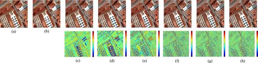
Figure 9. Comparison of fusion results on the Pavia University dataset. (a) Reference Image;
(b) LR-HSI; (c) CNMF; (d) HySure; (e) NLSTF; (f) CSTF; (g) UTV-HSISR; (h) JRLTD
From Figure 9, we can see that the spatial details in the fusion results of different
methods are greatly enhanced. However, compared with the reference image, there are still
some spectral differences and noise effects in the fused image. For example, in Figure 9c,d,
the fusion results of CNMF [29] and Hysure [18] show spectral distortion. Compared with
the fusion results in Figure 9e,f, the fused images in Figure 9g,h are able to provide better
spectral information and preserve the spatial structure.
In addition, it can be seen from the difference images that the reconstruction errors is
relatively large from the difference images of Figure 9c–e. Figure 9g,h are better and similar
compared with Figure 9f. In other words, the UTV-HSISR algorithm [41] and the JRLTD
algorithm proposed in the paper achieve better fusion results, that is, there is little noise.
The quality indicators of the comparison method are shown in Table 2, and the better
results obtained in the experiment are highlighted in bold typeface. From the spectral
features, the algorithm proposed in this paper has the smallest RMSE, the closest CC to 1,
the smallest ERGAS, the smallest SAM, and the smallest DD, indicating that the algorithm
proposed in this paper is closest to the reference image, has the smallest spectral distortion,
and has the best spectral agreement with the reference image. From the results of signal-
to-noise ratio, the algorithm in this paper has the highest PSNR, which indicates that the
algorithm has the best effective suppression of noise. From the spatial characteristics, SSIMRemote Sens. 2021, 13, 4116 16 of 27
is closest to 1, indicating that it is closest to the reference image in terms of brightness,
contrast and structure; UIQI is closest to 1, indicating that the loss of relevant information
reaches the minimum, the closer to the reference image.
Table 2. Quality evaluation for Pavia University dataset.
Spectral Features Signal-To-Noise Ratio Spatial Features
Methods
RMSE CC ERGAS SAM DD PSNR SSIM UIQI
BEST 0 1 0 0 0 ∞ 1 1
CNMF 6.3889 0.9702 3.6300 3.7427 3.9586 32.1227 0.9366 0.9492
HySure 4.0104 0.9880 2.2397 3.3363 2.5411 36.4850 0.9703 0.9790
NLSTF 2.0265 0.9966 1.1602 2.0873 1.3064 44.4323 0.9706 0.9928
CSTF 1.7673 0.9974 0.9886 1.8391 1.1610 43.9473 0.9881 0.9942
UTV-HSISR 1.6881 0.9976 0.9294 1.7635 1.0460 44.6407 0.9898 0.9950
Proposed 1.6552 0.9977 0.9072 1.7097 1.0105 44.8388 0.9905 0.9952
4.5.2. Experiment on Washington DC
In order to better display more spatial detail information and fusion results, we select
three bands(R:40, G:30, B:5) to be synthesized as pseudo-color image for display, and then
compared with other methods, the fusion results of Washington DC dataset are shown in
the first row of Figure 10. Besides, in order to show the fusion performance more visually,
we generate difference images to present the discrepancy between the reference image
and the fused image. The second row of Figure 10 shows the difference image of the
Washington DC dataset.
Figure 10. Comparison of fusion results on the Washington DC dataset. (a) Reference Image;
(b) LR-HSI; (c) CNMF; (d) HySure; (e) NLSTF; (f) CSTF; (g) UTV-HSISR; (h) JRLTD.
It can be seen that the spectral information is distorted in the results of CNMF [29]
and HySure [18]. In addition, there are some blurring effects in the building regions in the
results of NLSTF [38] when compared with Figure 10a. Compared with the fusion results
of CSTF [39], the fused images of UTV-HSISR [41] and JRLTD are able to provide better
spectral information and preserve the spatial structure. From the difference images, we can
observe that the error of the UTV-HSISR algorithm [41] and the JRLTD algorithm proposed
in the paper is smaller as a whole.
The quality evaluation results are shown in Table 3, and the better values obtained in
the experiment are marked with bolded font. From Table 3, it can be seen that the algorithm
proposed in this paper has the smallest RMSE, the closest CC to 1, the second minimum
value of ERGAS, the smallest SAM, and the smallest DD in terms of spectral features.
Collectively, the algorithm proposed in this paper is the closest to the reference image, with
the smallest spectral distortion and the best spectral agreement with the reference image.
From the results of signal-to-noise ratio, the algorithm in this paper has the highest PSNR,
which indicates that the algorithm has the best effective suppression of noise. From the
spatial characteristics, SSIM is closest to 1, which indicates that it is closest to the reference
image in terms of brightness, contrast and structure; UIQI is closest to 1, which indicates
that the loss of relevant information reaches the minimum, the closer to the reference image.Remote Sens. 2021, 13, 4116 17 of 27
In summary, the JRLTD algorithm proposed in this paper outperforms other algorithms in
most cases.
Table 3. Quality evaluation for Washington DC dataset.
Spectral Features Signal-To-Noise Ratio Spatial Features
Methods
RMSE CC ERGAS SAM DD PSNR SSIM UIQI
BEST 0 1 0 0 0 ∞ 1 1
CNMF 4.1122 0.9745 3.4984 3.2825 2.9279 37.5546 0.9585 0.9569
HySure 3.0588 0.9837 3.7441 3.4822 1.9632 39.7109 0.9778 0.9749
NLSTF 1.2778 0.9947 2.2339 1.7381 0.7840 48.1596 0.9923 0.9919
CSTF 1.0618 0.9950 2.3983 1.5433 0.6865 48.3925 0.9945 0.9926
UTV-HSISR 0.9397 0.9962 2.0301 1.3421 0.5444 49.7023 0.9961 0.9945
Proposed 0.8847 0.9963 2.0478 1.2454 0.4871 50.2731 0.9966 0.9946
4.5.3. Experiment on Sand Lake in Ningxia of China
In order to better display more spatial detail information and fusion results, we select
three bands (R:41, G:25, B:3) to be synthesized as pseudo-color image for displaying,
respectively, and then compared with other methods, the fusion results of Sand Lake
dataset are shown in the first row of Figure 11. In addition, to show the fusion performance
more visually, we generate difference images to present the discrepancy between the
reference image and the fused image. The second row of Figure 11 shows the difference
image of the Sand Lake dataset.
Figure 11. Comparison of fusion results on the Sand Lake dataset. (a) Reference Image; (b) LR-HSI;
(c) CNMF; (d) HySure; (e) NLSTF; (f) CSTF; (g) UTV-HSISR; (h) JRLTD.
After corresponding the fusion results obtained in the first row of Figure 11 using dif-
ferent algorithms with the difference images in the second row, we can see that Figure 11c–e
have spectral distortion compared to the reference image. In addition, we can observe that
the Figure 11c–e are poorly reconstructed, so the difference images seems to have a lot of
information. From the difference images, Figure 11g,h are better and similar compared
to Figure 11f. In other words, the UTV-HSISR algorithm [41] and the JRLTD algorithm
proposed in the paper achieve better fusion results, that is, there is little noise.
Furthermore, Table 4 displays the quantitative experimental evaluations with eight
metrics. The better values obtained in the experiment are indicated in bold. As can be
seen from Table 4, from the spectral features, the algorithm proposed in this paper has
the smallest RMSE, the smallest ERGAS, the smallest SAM, the smallest DD, and CC
values are the same as those obtained by the UTV-HSISR algorithm. Overall, it shows that
the algorithm proposed in this paper is closest to the reference image, has the smallest
spectral distortion, and has the best spectral agreement with the source image. From the
results of the signal-to-noise ratio, the algorithm in this paper has the highest PSNR, which
indicates that the algorithm has the best effective suppression of noise. From the spatial
characteristics, SSIM is closest to 1, which indicates that it is closest to the reference image
in terms of brightness, contrast and structure; UIQI is closest to 1, which indicates that the
loss of relevant information reaches the minimum, the closer to the reference image. InRemote Sens. 2021, 13, 4116 18 of 27
general, the JRLTD algorithm proposed in this paper outperforms other algorithms in most
cases.
Table 4. Quality evaluation for Sand Lake dataset.
Spectral Features Signal-To-Noise Ratio Spatial Features
Methods
RMSE CC ERGAS SAM DD PSNR SSIM UIQI
BEST 0 1 0 0 0 ∞ 1 1
CNMF 3.5512 0.9752 1.1293 1.1495 2.4822 37.6549 0.9681 0.9688
HySure 2.9776 0.9935 1.8847 1.3881 1.9273 39.6945 0.9732 0.9820
NLSTF 2.0026 0.9965 0.6263 1.1535 1.4592 44.4597 0.9841 0.9828
CSTF 1.5303 0.9980 0.4853 0.9782 1.1343 44.7850 0.9860 0.9859
UTV-HSISR 0.8926 0.9994 0.2932 0.5514 0.5054 50.5421 0.9956 0.9959
Proposed 0.8452 0.9994 0.2786 0.5191 0.4606 51.0214 0.9962 0.9965
5. Conclusions
In this paper, a hyperspectral image super-resolution method using joint regularization
as prior information is proposed. Considering the geometric structures of LR-HSI and
HR-MSI, two graphs are constructed to capture the spatial correlation of HR-MSI and the
spectral similarity of LR-HSI. Then, the presence of anomalous noise values in the images
was reduced by smoothing the LR-HSI and HR-MSI using unidirectional total variational
regularization. In addition, an optimization algorithm based on PAO and ADMM is
utilized to efficiently solve the fusion model. Finally, experiments were conducted on two
benchmark datasets and one real dataset. Compared with some fusion methods such as
CNMF [29], HySure [18], NLSTF [38], CSTF [39], and UTV-HSISR [41], this fusion method
produces better spatial details and better preservation of the spectral structure due to the
superiority of joint regularization and tensor decomposition.
However, there are still some limitations, and there is room for improvement of
the proposed JRLTD algorithm. For example, the proposed JRLTD algorithm has a high
computational complexity, and this leads to a relatively long running time. In our future
work, we aim to extend the method in two directions. On the one hand, since the model
utilizes the ADMM algorithm, although it is possible to divide a large complex problem into
multiple smaller problems that can be solved simultaneously in a distributed manner, leads
to an increase in computational effort and a decrease in computational speed. Therefore,
we will try to find a closed form solution for each sub-problem. Alternatively, it can be
accelerated by using parallel computing techniques. On the other hand, there is non-local
spatial similarity in HSI, that is, there are duplicate or similar structures in the image,
and when processing blocks of images, we can use information from surrounding blocks
of images that are similar to them. This prior information has been shown to be valid
for image super-resolution problems. Therefore, we will investigate the incorporation of
non-local spatial similarity into the JRLTD method.
Author Contributions: Funding acquisition, W.B.; Validation, K.Q.; Writing—original draft, M.C.;
Writing—review & editing, W.B. All authors have read and agreed to the published version of the
manuscript.
Funding: This work is supported by the Natural Science Foundation of Ningxia Province of China
(Project No. 2020AAC02028), the Natural Science Foundation of Ningxia Province of China (Project
No. 2021AAC03179) and the Innovation Projects for Graduate Students of North Minzu University
(Project No.YCX21080).
Acknowledgments: The authors would like to thank the Key Laboratory of Images and Graphics
Intelligent Processing of State Ethnic Affairs Commission: IGIPLab for their support.
Conflicts of Interest: The authors declare no conflict of interest.You can also read