Comparing LSTM and GRU for Multiclass Sentiment Analysis of Movie Reviews - Pawan Kumar Sarika
←
→
Page content transcription
If your browser does not render page correctly, please read the page content below
Bachelor of Science in Computer Science
February 2018

   Comparing LSTM and GRU for
Multiclass Sentiment Analysis of Movie
               Reviews.

                          Pawan Kumar Sarika

  Faculty of Computing, Blekinge Institute of Technology, 371 79 Karlskrona, Sweden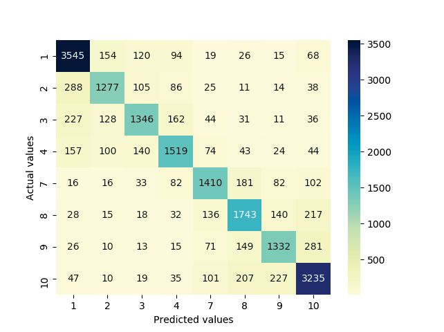
This thesis is submitted to the Faculty of Computing at Blekinge Institute of Technology in
partial fulfilment of the requirements for the degree of Bachelor of Science in Computer Science.
The thesis is equivalent to 10 weeks of full time studies.

The authors declare that they are the sole authors of this thesis and that they have not used
any sources other than those listed in the bibliography and identified as references. They further
declare that they have not submitted this thesis at any other institution to obtain a degree.

Contact Information:
Author(s):
Pawan Kumar Sarika
E-mail: pasr19@student.bth.se

University advisor:
Dr. Prashant Goswami
Department of Computer Science

Faculty of Computing                               Internet : www.bth.se
Blekinge Institute of Technology                   Phone    : +46 455 38 50 00
SE–371 79 Karlskrona, Sweden                       Fax      : +46 455 38 50 57
Abstract

Today, we are living in a data-driven world. Due to a surge in data generation,
there is a need for efficient and accurate techniques to analyze data. One such kind
of data which is needed to be analyzed are text reviews given for movies. Rather
than classifying the reviews as positive or negative, we will classify the sentiment of
the reviews on the scale of one to ten. In doing so, we will compare two recurrent
neural network algorithms Long short term memory(LSTM) and Gated recurrent
unit(GRU).
    The main objective of this study is to compare the accuracies of LSTM and
GRU models. For training models, we collected data from two different sources. For
filtering data, we used porter stemming and stop words. We coupled LSTM and
GRU with the convolutional neural networks to increase the performance.
    After conducting experiments, we have observed that LSTM performed better in
predicting border values. Whereas, GRU predicted every class equally. Overall GRU
was able to predict multiclass text data of movie reviews slightly better than LSTM.
GRU was computationally expansive when compared to LSTM.

Keywords: Gated recurrent unit, Multiclass classification, Movie reviews, Senti-
ment Analysis, Recurrent neural network,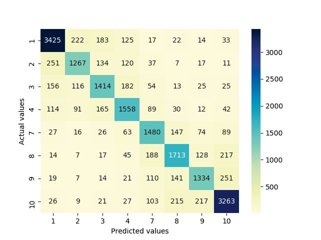

Acknowledgments

I would like to dedicated my dissertation to my parents because of there unfailing
support. Many deepest appreciations to my supervisor Dr. Prashant Goswami , who
guided me through every step of my thesis.
    I would also like to thank all the doctors and front-line workers who risked there
lives to keep us safe during the period of corona virus pandemic.
                                                                 Pawan Kumar Sarika

                                          iii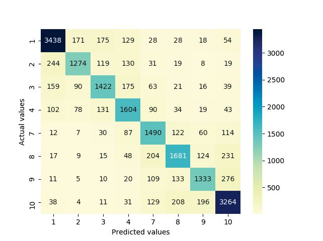
Contents

Abstract                                                                                                                               i

Acknowledgments                                                                                                                      iii

1 Introduction                                                                                                                        1
  1.1 Background . . . . . . . . . . . . . . . . . . . . . . . . . . . . . . . .                                                      2
       1.1.1 Neural Networks . . . . . . . . . . . . . . . . . . . . . . . . .                                                        2
  1.2 Aim and scope . . . . . . . . . . . . . . . . . . . . . . . . . . . . . .                                                       6

2 Related Work                                                                                                                        7

3 Method                                                                                                                              9
  3.1 Datasets . . . . . . . . . .   .   .   .   .   .   .   .   .   .   .   .   .   .   .   .   .   .   .   .   .   .   .   .   .    9
      3.1.1 Dataset 1 . . . . .      .   .   .   .   .   .   .   .   .   .   .   .   .   .   .   .   .   .   .   .   .   .   .   .   10
      3.1.2 Dataset 2 . . . . .      .   .   .   .   .   .   .   .   .   .   .   .   .   .   .   .   .   .   .   .   .   .   .   .   11
      3.1.3 Final datasets . . .     .   .   .   .   .   .   .   .   .   .   .   .   .   .   .   .   .   .   .   .   .   .   .   .   11
  3.2 Pre-Processing Algorithms      .   .   .   .   .   .   .   .   .   .   .   .   .   .   .   .   .   .   .   .   .   .   .   .   12
      3.2.1 Filtering text . . .     .   .   .   .   .   .   .   .   .   .   .   .   .   .   .   .   .   .   .   .   .   .   .   .   12
      3.2.2 Porter Stemming .        .   .   .   .   .   .   .   .   .   .   .   .   .   .   .   .   .   .   .   .   .   .   .   .   13
      3.2.3 Stop Words . . . .       .   .   .   .   .   .   .   .   .   .   .   .   .   .   .   .   .   .   .   .   .   .   .   .   13
  3.3 Experimental setup . . . .     .   .   .   .   .   .   .   .   .   .   .   .   .   .   .   .   .   .   .   .   .   .   .   .   14
  3.4 Data Visualization . . . .     .   .   .   .   .   .   .   .   .   .   .   .   .   .   .   .   .   .   .   .   .   .   .   .   16

4 Results and Analysis                                                                                                               19
  4.1 Experiment 1 . . . . . . . . . . . . . . . . . . . . . . . . . . . . . . .                                                     19
  4.2 Experiment 2 . . . . . . . . . . . . . . . . . . . . . . . . . . . . . . .                                                     20
  4.3 Experiment 3 . . . . . . . . . . . . . . . . . . . . . . . . . . . . . . .                                                     23

5 Discussion                                                                                                                         25

6 Conclusions and Future Work                                                                                                        27

References                                                                                                                           29

A Supplemental Information                                                                                                           31

                                                 v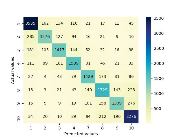
List of Figures

1.1   Simple Neural network Structure . . . . . . . . . . . . . . . . . . . .                            3
1.2   Internal structure of Long Short Term Memory [3] . . . . . . . . . . .                             4
1.3   Internal structure of Gated Recurrent Unit[3] . . . . . . . . . . . . .                            6

3.1   Final Dataset count . . . . . . . . . . . . . . . . . . . . . . . . . . . .                        12
3.2   Line Graph for Accuracy . . . . . . . . . . . . . . . . . . . . . . . . .                          17
3.3   Confusion matrix heat map . . . . . . . . . . . . . . . . . . . . . . .                            17

4.1   Confusion matrix heat map for Porter Stemming .        .   .   .   .   .   .   .   .   .   .   .   20
4.2   Confusion matrix heat map for Stop Words . . . .       .   .   .   .   .   .   .   .   .   .   .   21
4.3   Confusion matrix heat map for Basic . . . . . . .      .   .   .   .   .   .   .   .   .   .   .   21
4.4   Accuracy line graph for Basic . . . . . . . . . . .    .   .   .   .   .   .   .   .   .   .   .   22
4.5   Accuracy line graph for Basic . . . . . . . . . . .    .   .   .   .   .   .   .   .   .   .   .   24

A.1 Accuracy Line graphs for Porter Stemming . . . . . . . . . . . . . . .                               31
A.2 Accuracy Line graphs for Stop words . . . . . . . . . . . . . . . . . .                              31
A.3 Accuracy Line graphs for 500 Epochs . . . . . . . . . . . . . . . . . .                              32

                                        vii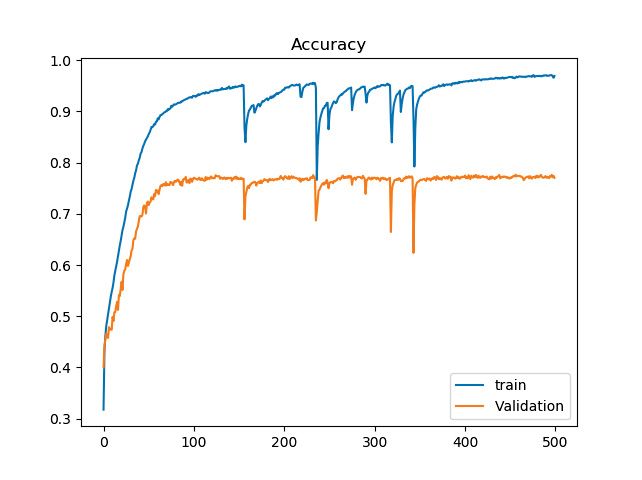
List of Tables

3.1   Sample Dataset . . . .    .   .   .   .   .    .   .   .   .   .   .   .   .   .   .   .   .   .   .   .   .   .   .   .   .   .   11
3.2   Python Packages . . .     .   .   .   .   .    .   .   .   .   .   .   .   .   .   .   .   .   .   .   .   .   .   .   .   .   .   14
3.3   Class labels for data .   .   .   .   .   .    .   .   .   .   .   .   .   .   .   .   .   .   .   .   .   .   .   .   .   .   .   15
3.4   Experiment Conducted      .   .   .   .   .    .   .   .   .   .   .   .   .   .   .   .   .   .   .   .   .   .   .   .   .   .   16

4.1   Experiment 1 Summary . . . . . . . . . . . . . . . . . . . . . . . . .                                                             19
4.2   Experiment 2 Summary . . . . . . . . . . . . . . . . . . . . . . . . .                                                             22
4.3   Experiment 3 Summary . . . . . . . . . . . . . . . . . . . . . . . . .                                                             23

5.1   Test dataset . . . . . . . . . . . . . . . . . . . . . . . . . . . . . . . .                                                       25

                                                    ix
Chapter 1
Introduction
Being in the digital world, we as humans constantly generate data knowingly or
unknowingly. Every time we use the internet it is most likely our activities generate
data in one way or another. Simple tasks like searching a keyword using a search
engine and opening relevant website generate data for the search engines. At first
glance, this data may seem useless but when we combine data of preferred website
by thousands of users for a single keyword, we can find the most popular or most
relevant website for that keyword which helps search engines to show relevant results.
This encourages every internet-based entity to collect data.
We are getting increasingly dependent on the internet. If we want to know the
meaning of a word, get to a location, send money or to search for a movie, we use
the internet. Because of this, there is a surge in data generation. To administer this
data there is a need for efficient and reliable data warehousing.
When a movie is released in theatres, television or online streaming sites (Amazon
Prime, Netflix, Hulu, etc.), some people who have watched the movie express their
views in the form of text (reviews). These reviews generally posted on websites such
as IMDB(internet movie database), rotten tomatoes. It is a common scenario when
a person wants to watch a movie they read reviews so they can have an insight into
the movie. But we cannot tell if the movie is good or bad by simply reading two
or three reviews. Following are the two contrasting reviews for the Oscar-winning
movie ’Parasite’ from IMDB website
Rating: 10/10
Review 1: "The most original film of 2019 and it is wickedly funny and darkly
disturbing all at the same time. The narrative and the actors were excellent. One of
the better endings of a movie in quite a while. Class warfare at its best" [14].
Rating: 1/10
Review 2: "When I find myself constantly looking at my watch and asking when
a film is going to deliver any of the promises that the Critics and Reviewers have
seen fit to lavish on it then there’s something awry. This isn’t scathing socio-political
cinema...it’s not black comedy, in fact it’s not remotely amusing or believable or even
sympathetic to any of its characters. It’s a simple hype job. The movie here is the
real Parasite" [14].
These contrast in reviews leads to a dilemma. Hence, we need to analyse a
significant number of reviews. If we analyze enough number of reviews, we can
12 Chapter 1. Introduction
classify the movie as good or bad. To be more precise we can classify the movie
reviews on the scale of one to ten, one being worst and ten being excellent. To mine
the opinion of the reviewer, there is a need for Sentiment analysis of text reviews.
Sentiment analysis focuses on the analysis and understanding of the emotions from
the text patterns. It identifies the opinion or attitude that a person has towards a
topic or an object, and it seeks to identify the viewpoint underlying a text span [20].
1.1 Background
Sentiment analysis of text appears to be a simple task for humans but when we
need to analyse thousands of text reviews at ones, sentiment analysis becomes a dif-
ficult and time-consuming task. This task can be automated using machine-learning
techniques. Machine learning techniques are the computer algorithms that improve
automatically through experience [2].
Using computer algorithms for sentiment analysis of text reviews can be a com-
plex task. The reviewer generally write reviews in their natural language. These text
reviews do not have a specific structure. When a human reads a sentence, he/she
tends to understand the whole sentence rather than looking at the words. For in-
stance, "The movie lacks good characters, simple plot, elegant theme, attention to
details and satisfactory ending." a human reader could easily tell this is a negative
review but for a computer this could be difficult to classify because when we look at
the words there are five words that depict positive sentiment whereas there is only
one word that depicts negative sentiment. Hence to classify the sentiments, in this
research we use Neural networks one the subset of machine learning.
1.1.1 Neural Networks
Neural networks are a set of algorithms which are designed in such a way that they
mimic a human brain. The execution of algorithms is similar to that of humans.
They try random things, learn from previous experience, improve and make decisions
accordingly.The ability of neural networks to learn can be key for sentiment analysis
of text reviews. As we need to learn the dependency of words on one another.
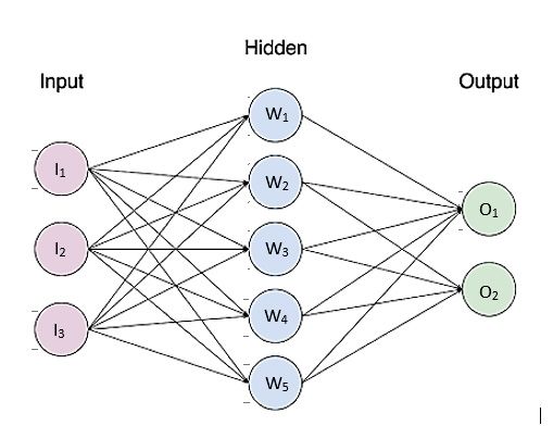
The figure 1.1 represents a simple neural network structure. Neural network
mainly constitutes of three layers, input layer, hidden layer and output layer. These
three layers are built-up of neurons. Input layer is the data that is provided. hidden
layer are the weights which are determined using special mathematical functions.
Output layer is the final result of the input data.
Among the vast variety of neural networks. In this report, we concentrated on
two variants of the recurrent neural network (LSTM and GRU).Recurrent Neural
network (RNN) is a class of neural networks which remembers every information
through time [22]. This is crucial as we need to understand the dependency of one
word on another. During the time of training models on LSTM and GRU, we have
observed that both the algorithms take 2-4 hours for each epoch. Due to the time
constraints, we coupled LSTM and GRU with a convolutional neural network(CNN).
This lead to a significant decrease in training time.1.1. Background 3
Figure 1.1: Simple Neural network Structure
In this research, we will conduct a study on two RNN algorithms, LSTM and it’s
variant GRU. We will try to classify text reviews of movies on the scale of one to ten
using LSTM and GRU and determine how they compare for sentiment analysis.
The reason for selecting LSTM is because the study [25] states that "Experimental
results show that the proposed method outperforms lexicon-based, regression-based,
and NN-based methods for the text data resembling valence-arousal". In another
study [18] which states "Each text is represented by a latent topic space instead of
a word space, and the ability to process long-term sequences by CNN is improved
by combining GRU, so as to achieve a highly accurate classifier". The reason for
selecting GRU is because the mentioned study stated that it improved their results.
Long Short Term Memory
Hochreiter and Schmidhuber initially proposed the long short term memory (LSTM)
in the year 1997 [13]. LSTM is a type of Recurrent Neural Network (RNN). RNN
neurons have a connection to the previous neuron state in addition to the layer
inputs. RNNs are particularly benefitial to data that is sequential or that can value
a contextual view. therefore, RNNs can be impressive in text classification [26]. RNN
remembers every information through time [22]. While working with gradient-based
learning algorithms we face an increasingly difficult problem, The problem occurs
when there is an increment in the duration of capturing the dependencies while
generating a model [6]. We can address this problem using Long short-term memory
(LSTM) [13].
LSTM consists of a memory cell to store information. It computes input gate,
forget gate and output gate to manage this memory. LSTM units can propagate an
important feature that came early in the input sequence over a long distance. Hence,
capturing potential long-distance dependencies [7]. Following equations computes
time-step t for each hidden state [3]:
Forget gate:
ft = σ(Wf · [ht−1 , xt ] + bf )4 Chapter 1. Introduction
Candidate layer:
it = σ(Wi · [ht−1 , xt ] + bi )
Input Gate:
C̃t = tanh(WC · [ht−1 , xt ] + bc )
Output Gate:
Ct = ft ∗ Ct−1 + it ∗ C̃t
Hidden state:
ot = σ(Wo [ht−1 , xt ] + bo )
Memory state:
ht = ot ∗ tanh(Ct )
Where W and b denotes weight vector for forget gate(f), scandidate(C), input
gate(i), output gate(o). ∗ denotes element wise multiplication and σ is the sigmoid
function. The figure 1.2 demonstrate the internal structure of LSTM at time-step t.
Figure 1.2: Internal structure of Long Short Term Memory [3]1.1. Background 5
Gated Recurrent Unit
Even though LSTM deals with the vanishing gradient problem, a generalised form
of LSTM [4] is Gated Recurrent Unit (GRU) which was proposed in 2014 by Cho et
al [11]. Similar to the LSTM unit, the GRU has gating units that modulate the flow
of information inside the unit, however, without having a separate memory cells.
Gated Recurrent Unit (GRU) calculates two gates called update and reset gates
which control the flow of information through each hidden unit. Each hidden state
at time-step t is computed using the following equations [7]:
Update gate:
zt = σ(Wz · [ht−1 , xt ])
Reset gate:
rt = σ(Wr · [ht−1 , xt ])
New memory:
h̃t = tanh(W · [rt ∗ ht−1 , xt ])
Final memory:
ht = (1 − zt ) ∗ ht−1 + zt ∗ h̃t
Where W denotes weight vector, ∗ denotes element wise multiplication and σ is
the sigmoid function. The figure 1.2 demonstrate the internal structure of LSTM at
time-step t.
Convolutional Neural Network
Convolutional neural networks (CNNs), are a specialized kind of neural network for
processing data that has a known grid-like topology, this was introduced by LeCun et.
al. in 1998 [17]. The name “convolutional neural network” indicates that the network
employs a mathematical operation called convolution. Convolution is a specialized
kind of linear operation. Convolutional networks are simply neural networks that use
convolution in place of general matrix multiplication in at least one of their layers
[12].
Even though CNNs were Originally invented for computer vision, the article by
Yoon Kim has shown that a simple CNN with one layer of convolution performs
remarkably well for convolutional neural networks built on top of word2vec [16]. In
this research, convolutional neural network is adopted to increase the performance of
LSTM and GRU. A study by Alec Yenter on CNN-LSTM has shown that performnce
vastly improves upon the baseline CNN-LSTM model [27].6 Chapter 1. Introduction
Figure 1.3: Internal structure of Gated Recurrent Unit[3]
1.2 Aim and scope
This research majorly focuses on the performance of LSTM and GRU in terms of
accuracy for classifying text reviews given for movies on the scale of one to ten. We
will try to answer the question:
• Which of the two, LSTM and GRU algorithms will have higher accuracy for
multi-class classification of supervised textual data of movie reviews?
To answer this question, we set four main objectives. these objectives will even-
tually help us to achieve our aim to compare the accuracy of LSTM and GRU for
text reviews. Following are the objectives:
1. Gathering data that can be used for training, validation and testing purposes.
2. Applying pre-processing to filter data.
3. Training and generating models using algorithms on supervised data of movie
reviews that predicts the class of the review.
4. Analizing the final models using validation and testing data and then comparing
the algorithms.
The sentiment analysis of movie reviews can be proven worthy for Blue-Ray
retailers, TV channels and streaming services like Netflix, Amazon, HBO, etc. These
entertainment services can use Sentiment analysis of the movie reviews to suggest
movies of higher rating to their customers.Chapter 2
Related Work
There are several pieces of research which when put together contribute to this study.
A paper ’Sentiment Analysis and Classification Based On Textual Reviews’ by
K.Mouthami proposed a new algorithm called Sentiment Fuzzy Classification algo-
rithm is proposed to improve classification accuracy on the benchmark dataset of
Movies reviews [20].
Even though the proposed method does not relate to our study, the problems
addressed and the type of data set is similar. This paper helped us to determine
several steps that are needed for sentiment classification approaches.
Architectures for text categorization and sentiment analysis[9] has shown the
importance of pre-processing in neural networks. In this paper, researchers analyzed
the impact of simple text pre-processing decisions on the performance of a standard
word-based neural text classifier. There evaluations highlight the importance of
being careful in the choice of how to pre-process our data and to be consistent when
comparing different systems.
The study state that there is a high variance in the results depending on the
pre-processing choice (±2.4% on average for the best performing model)[9]. This
study motivated us to investigate several pre-processing techniques which lead us to
the next study.
V. Srividhya evaluated three important pre-processing techniques namely, stop
word removal, stemming and TF/IDF on Reuters dataset[23]. This study has shown
that pre-processing has a huge impact on performances of classification. From this
study we have Incorporated two pre-processing techniques stop word removal and
stemming.
The paper on sentiment analysis with gated recurrent units by Shamim Biswas is
a major contributor to our research. In this paper, researchers did sentiment analysis
at the paragraph level of movie reviews as positive or negative. Different approaches
used by us are Tf-idf, Word2Vec (vector average), Word2Vec (k – means dictionary),
GRU (gated recurrent units) and Ensemble model. and concluded that conclude
that gated recurrent units are a suitable model for sentiment analysis especially at
the paragraph level[7].
In our research, we will compare LSTM and GRU for multiclass sentiment analysis
and will try to find out model with higher accuracy. we will also incorporate and
test different pre-processing techniques.
Hadi Pouransari in his study ’Deep learning for sentiment analysis of movie re-
views’ implemented the recursive neural tensor networks(RNTN) to train a multi-
class sentiment analyzer. The training of standard RNTN was computationally very
78 Chapter 2. Related Work
expensive. To overcome the high computational cost of training the standard RNTN
we introduce the lowrank RNTN, in which the matrices involved in the quadratic
term of RNTN are substituted by symmetric low-rank matrices. We show that the
low-rank RNTN leads to significant saving in computational cost, while having sim-
ilar a accuracy as that of RNTN[21]. This study has shown how we can apply
sentiment analysis on multiclass text data using neural networks.
A blog post on sequence classification with LSTM Recurrent Neural Networks in
Python with Keras by Jason Brownlee[8] has shown the addition of convolutional
layer to LSTM reduce the training time of LSTM without affecting the accuracy.
Due to the time constrains we have incorporated this method.Chapter 3
Method
To obtain a solution to the research question, the method used is a formal exper-
iment. In a formal experiment, we create identical circumstances to test methods,
activities, Algorithms, etc. to identify what effect they have. Artificial neural net-
works are a good example of the explorative mode of experimentation. After having
been discarded on theoretical grounds, experiments demonstrated properties bet-
ter than predicted [24]. For this project, We experiment on the LSTM and GRU
Recurrent neural network algorithm which comes under Artificial neural networks,
experimentation is better fitted.
To determine which of the two LSTM or GRU has algorithm has higher accuracy
for multiclass classification of text data. We used text reviews given to the movies
by the users. Here the reviews are classified into the scale of one to ten. We are
adopting LSTM and GRU as a tool to processes the natural language of text reviews
given to the movies. We generated separate models for each method using training
data from the dataset. The models are then used to predict the class of reviews. We
compare the predicted values to actual values in the test data to determine accuracy.
In the experiment, we also used Porter stemming and Stop words (Natural language
processing tools) to filter data. To improve the efficiency of LSTM and GRU, we
coupled them with the convolutional neural network.
Further this chapter comprises details regarding Datasets, Algorithms, Experi-
mental setup and Visualization techniques employed in this experiment.
3.1 Datasets
To train and test the RNN model for text reviews of movies to classify them from
one to ten, There is a need for a large amount of data. Firstly we used Large movie
review dataset V1.0 by Andrew L. Maas [19]. This dataset has a total of 50,000 IMDB
movie reviews classified into positive and negative data. For more data, we included
another dataset of kaggle’s Bag of Words Meets Bags of Popcorn competition [1].
This dataset also has 50,000 IMDB movie reviews evenly distributed into Train and
Test data.
Both the dataset are primarily meant for binary classification (positive or neg-
ative) of movie reviews. Since the aim is to predict multiclass sentiments of movie
reviews, the dataset is also needed to be classified into multiclass (Scale of one to
ten). Fortunately, both the datasets have unique ids for each review which incor-
porate a rating from one to ten given by the user while writing the review. For
example, In the dataset by Andrew Maas, ’11867_8.txt’ is a file containing a single
910 Chapter 3. Method
review. We can observe that the file name has two attributes separated by an under-
score, ’11867’ refers to review id and ’8’ refers to the rating. Hence, to extract rating
from the dataset we used python to automate the process. Section 3.1.1 Describes
extraction process for Large movie review dataset V1.0 by Andrew L. Maas [19].
Section 3.1.2 Describes extraction process for kaggle’s Bag of Words Meets Bags of
Popcorn competition [1].Section 3.1.3 contains details of final dataset that is used
for training and testing.
3.1.1 Dataset 1
In Dataset 1 there are two top-level directories [train/, test/] corresponding to the
training and test sets. Each contains [pos/, neg/] directories for the reviews with
binary labels positive and negative. Within these directories, reviews are stored in
text files named following the convention [[id]_[rating].txt] where [id] is a unique id
and [rating] is the star rating for that review on a 1-10 scale. For example, the file
[test/pos/200_8.txt] is the text for a positive-labeled test set example with unique
id 200 and star rating 8/10 from IMDb [19].
Firstly we manually copied every txt files in train and test directories into a single
directory. While manually copying the file into a single directory, some of the files
which may have some identical file name with different contents are renamed by
default. We use code in Listing 3.1 to read and store names of each file to extract
rating from the file name. The code in Listing 3.2 extracts ratings from the file names
and also stores them in a new file along with the reviews. The new file consists of
two columns ’Sentiment’ and ’Review’.
1 # directory holding all files
2 mypath = os . path . join ( mypath , " Combined_data " )
3 for ( dirpath , dirnames , filenames ) in walk ( mypath ) :
4 # Adding all file name to the list
5 filelist . extend ( filenames )
Listing 3.1: Retrieving file names
1 for i in filelist :
2 # Splitting file extension ( txt )
3 filename_complete = i . split ( " . " )
4 # Splitting id
5 filename_splited = filename_complete [0]. split ( " _ " )
6 if ( ’ ’ in filename [1]) :
7 # Splitting rating if file is renamed
8 renamed = filename_splited [1]. split ( " " )
9 Sentiment = renamed [0]
10 else :
11 Sentiment = filename_splited [1]
12 filename = os . path . join ( mypath , i )
13 file = open ( filename , " r " , encoding = " utf -8 " )
14 # writing sentiments and reviews in a new file
15 newdataset . write ( " \" " + Sentiment + " \"\ t " + " \" " + file . read () + " \"\ n " )
16 file . close ()
Listing 3.2: Seprating rating from filename3.1. Datasets 11
3.1.2 Dataset 2
The Dataset 2 consist of two files ’labeledTrainData.tsv’ and ’testData.tsv’. Both the
file contain 25,000 reviews each and has three columns ’id’, ’sentiment’, ’review’. In
this dataset, the rating that is needed to be extracted are present in the ’id’ column.
every row of ’id’ column follows the convention [[id]_[rating]] where [id] is a unique
id and [rating] is the star rating for that review on a 1-10 scale.
We used the code in Listing 3.3 to extract ratings from the ’id’ column. After
extracting we again store the ratings and reviews into a new file under the column
name ’Sentiment’ and ’Review’.
1 # Read from file
2 data_test = pd . read_csv ( Filename , delimiter =" \ t " , encoding = " utf -8 " )
3 # Separating rating from the id
4 data_test [ " sentiment " ] = data_test [ " id " ]. map ( lambda x : int ( x . strip ( ’
" ’) . split ( " _ " ) [1]) )
5 for i , j in data_test . iterrows () :
6 # writing sentiments and reviews in a new file
7 newdataset . write ( " \" " + str ( j [ " sentiment " ]) + " \"\ t " + " \" " + str ( j [ "
review " ]) + " \"\ n " )
Listing 3.3: Seprating rating from id
3.1.3 Final datasets
After combining data from dataset 1 and 2 we generate a new dataset which consists
of 100,000 samples. After combining the dataset we shuffle the rows randomly to
avoid any bias or patterns. The table 3.1 depicts a sample of the final dataset.
sentiment review
1 Just a stilted rip-off of the infinitely better...
10 This has to be the all time best computer...
7 Ok, so it may not be the award-winning...
2 I loved the first movie, the second one was...
3 Pretty poor Firestarter clone that seems more...
Table 3.1: Sample Dataset
Since the Both the parent datasets are for binary classification, they does not
have neutral reviews, which means they have excluded reviews with rating ’5’ and
’6’. Hence the final dataset also does not have any reviews with ratings ’5’ and ’6’.
Therefore, there are eight different classes (1,2,3,4,7,8,9,10) of reviews in the final
dataset. the figure 3.1 shows the count of each class for reviews.
We divide the final dataset two sets for training and testing. The training dataset
has 80% of total data i.e 80,000 samples, the testing dataset holds the rest of the
20,000 samples. We again divide 80% of the training dataset into training (64,000)
and validation dataset (16,000).12 Chapter 3. Method
Figure 3.1: Final Dataset count
3.2 Pre-Processing Algorithms
This section consists of details about methods used for data pre-processing. Since
we are dealing with text reviews that are written by the humans in there natural
language, the text reviews may or may not be structured. Hence, there is a need for
pre-processing text reviews. The study on the role of text pre-processing in neural
network architectures has shows that there is a high variance in the results depending
on the pre-processing choice [9].
To make all the text reviews uniform, we apply several filters like converting text
into lowercase, removing HTML tags, etc. I this experiment we also test Porter
Stemming and Stop Words techniques.
3.2.1 Filtering text
The text reviews in the dataset contains HTML tags.for example,
"This German horror film has to be one of the weirdest I have seen.I
was not aware of any connection between child abuse and vampirism"
The above review consist of HTML tag ’’, which does not have any sig-
nificance. Hence, HTML tags can be excluded, following is the processed text for
above example.
"This German horror film has to be one of the weirdest I have seen. I was not aware
of any connection between child abuse and vampirism"
Similarly, We Replace or convert characters which are insignificant. For this3.2. Pre-Processing Algorithms 13
experiment we convert all the reviews into lower case, replace digits with the text
’number’ and removing all the punctuation’s with spaces. Here is an example,
Review:
"I first viewed They Died With There Boots On,about 1970 and though it has been
many years since,this film and its impression remain."
Processed Review:
"i first viewed they died with there boots on about number and though it has been
many years since this film and its impression remain"
3.2.2 Porter Stemming
Online reviews are generally used with informal language and they include internet
slang and contemporary spellings like use of apostrophes, ing form of words to name
a few. So such words must be re-visited and stemmed for correct data retrieval [5].
Porter stemming is a technique used to extract the root of words by eliminating
suffixes like ’ing’, ’ly’, ’s’ etc. based on a rule. In this experiment we used PorerSrem-
mer in nltk(Natural Language Toolkit) library for python language. Following is an
example for porter stemming,
Review:
"what s inexplicable firstly the hatred towards this movie it may not be the greatest
movie of all time but gimme a break it got number oscars for a reason it made
eighteen hundred million dollars for a reason it s a damn good movie which brings to
the other inexplicable aspect of it i have no idea whatsoever why this movie left such
an impression on me when i saw it in theaters"
Processed Review:
"what s inexplic firstli the hatr toward thi movi it may not be the greatest movi of
all time but gimm a break it got number oscar for a reason it made eighteen hundr
million dollar for a reason it s a damn good movi which bring to the other inexplic
aspect of it i have no idea whatsoev whi thi movi left such an impress on me when i
saw it in theater"
3.2.3 Stop Words
Many of the most frequently used words in English are useless in Information Re-
trieval (IR) and text mining. These words are called ’Stop words’. Stop-words, which
are language-specific functional words, are frequent words that carry no information
(i.e., pronouns, prepositions, conjunctions) [23]. Examples of such words include
’the’, ’of’, ’and’, ’to’.
Review:
"i have to say i quite enjoyed soldier russell was very good as this trained psychopath
rediscovering his humanity very watchable and nowhere near as bad as i d been led
to believe yes it has problems but provides its share of entertainment"14 Chapter 3. Method
Processed Review:
"say quite enjoyed soldier russell good trained psychopath rediscovering humanity
watchable nowhere near bad led believe yes problems provides share entertainment"
3.3 Experimental setup
The experimental setup is to generate and test models for text review classification
using LSTM and GRU Recurrent neural networks. All the experiments are carried
on identical hardware and operating system.
Operating System: Windows 10 Education 64-bit (10.0, Build 18363)
System Manufacturer: Dell Inc.
System Model: Precision 5720 AIO
Processor: Intel(R) Xeon(R) CPU E3-1275 v6 @ 3.80GHz (8 CPUs), ∼3.8GHz
Memory: 16384MB RAM (16 GB)
GRU: Radeon (TM) Pro WX 7100 Graphics
Models are generated and teased in Python 3.7.6 environment. List of several
library functions used are given in table 3.2.
Package name Version
Keras 2.3.1
matplotlib 3.1.3
nltk 3.4.5
numpy 1.18.3
pickle 4.0
pandas 1.0.1
re 2.2.1
sklearn 0.20.3
tensorflow 1.14.0
Table 3.2: Python Packages
In section 3.1.3 we have seen that there are eight different classes (1,2,3,4,7,8,9,10),
we can observe that class labels are not continues. Since we need to define output
parameters, we modify the class labels to be continues. Modified class labels are
shown in table 3.3.
We will be using Using keras open-source neural-network library [10] for generat-
ing models. The keras only takes real numbers as input, hence we need to vectorise
data (converting words into numbers). In order to do so we first tokenize the data,
We tokenize text review given for movies using 5000 most frequently occurred words.
The tokenized words are then vectorised, following example demonstrate how this
is done. We apply sequence padding of 500 to ensure each reviews are are of same
length.
Review:3.3. Experimental setup 15
Class lable New Class lable
1 0
2 1
3 2
4 3
7 4
8 5
9 6
10 7
Table 3.3: Class labels for data
"This movie is amazing because the fact that the real people portray themselves
and their real life experience and do such a good job it’s like they’re almost living the
past over again."
Tokenised Review:
’This’, ’movie’, ’is’, ’amazing’, ’because’, ’the’, ’fact’, ’that’, ’the’, ’real’, ’people’,
’portray’, ’themselves’, ’and’, ’their’, ’real’, ’life’, ’experience’, ’and’, ’do’, ’such’, ’a’,
’good’, ’job’, "it’s", ’like’, "they’re", ’almost’, ’living’, ’the’, ’past’, ’over’, ’again.’
Vectorise Review:
[4, 5, 6, 7, 8, 1, 9, 10, 1, 2, 11, 12, 13, 3, 14, 2, 15, 16, 3, 17, 18, 19, 20, 21, 22,
23, 24, 25, 26, 1, 27, 28, 29]
Keras sequential is needed to be compiled after defining features, Listing 3.4
describe how the model was generated and tested. Convolutioal layer and Pooling
layer are add to increase the performance the Model.
1 model = Sequential ()
2 # Embedding layer
3 model . add ( Embedding ( input_dim = 5000 ,
4 output_dim = 32 ,
5 input_length = 512) )
6 model . add ( Dropout (0.2) )
7 # Convolutional layer
8 model . add ( Conv1D ( filters = 32 , kernel_size = 3 ,
9 padding = ’ same ’ ,
10 activation = ’ relu ’) )
11 # Pooling layer
12 model . add ( MaxPool1D ( pool_size = 2) )
13 if lstm == True :
14 # LSTM layer
15 model . add ( LSTM (256) )
16 else :
17 # GRU layer
18 model . add ( GRU (256) )
19 model . add ( Dropout (0.2) )16 Chapter 3. Method
20 model . add ( Dense (8 , activation = ’ softmax ’) )
21 model . compile ( loss = ’ c a t e g o r i c a l _ c r o s s e n t r o p y ’ ,
22 optimizer = ’ adam ’ , metrics = [ ’ accuracy ’ ])
23 # Training model on training data
24 model . fit ( x_train_data , y_train_data ,
25 batch_size =128 , epochs =100 ,
26 validation_data =[ x_val_data , y_val_data ])
27 # Making predictions for test data
28 prediction = model . predict_classes ( x_test_data , batch_size =64)
Listing 3.4: Keras model
We have conducted 18 different tests, table 3.4 lists tests conducted with different
arguments.
S.No. Model Pre-processing Epochs CNN layer
1 LSTM Porter Stemming 10 No
2 LSTM Stop Word 10 No
3 LSTM Basic 10 No
4 GRU Porter Stemming 10 No
5 GRU Stop Word 10 No
6 GRU Basic 10 No
7 LSTM Porter Stemming 200 Yes
8 LSTM Stop Word 200 Yes
9 LSTM Basic 200 Yes
10 GRU Porter Stemming 200 Yes
11 GRU Stop Word 200 Yes
12 GRU Basic 200 Yes
13 LSTM Porter Stemming 500 Yes
14 LSTM Stop Word 500 Yes
15 LSTM Basic 500 Yes
16 GRU Porter Stemming 500 Yes
17 GRU Stop Word 500 Yes
18 GRU Basic 500 Yes
Table 3.4: Experiment Conducted
3.4 Data Visualization
Data visualization is the representation of data or information in a graph, chart, or
other visual format. It communicates relationships of the data with images. This is
important because it allows trends and patterns to be more easily seen. With the
rise of big data upon us, we need to be able to interpret increasingly larger batches
of data. Machine learning makes it easier to conduct analyses such as predictive
analysis, which can then serve as helpful visualizations to present [15].
In this research, line chart and confusion matrix heat map is used for data vi-
sualization. Figure 3.2 is a sample of line graph which plots accuracy (y-axis) for
training data and validation data with respect to each epoch (x-axis). Figure 3.33.4. Data Visualization 17
visualizes confusion matrix for actual (y-axis) versus predicted (x-axis) values of test
data.
Figure 3.2: Line Graph for Accuracy
Figure 3.3: Confusion matrix heat mapChapter 4
Results and Analysis
In this chapter, the outcomes of each test is placed together. We divided all the tests
listed in table 3.4 into three sets based on number of epochs. Tests 1-6 are addressed
in section 4.1, tests 7-12 are addressed in section 4.2 and tests 13-18 are addressed
in section 4.3.
4.1 Experiment 1
This section consists of the tests that were conducted without the convolutional
layer. This test is conducted to check the computational cost of LSTM and GRU.We
conducted a similar test, where LSTM and GRU are coupled with convolutional
neural network.
The table 4.1 illustrates average training time for each epochs and accuracy
achieved after ten epochs on test data for the simple model and model coupled
with CNN.
Training
Training
Time per Test data
S. Time per Test data
Model Pre-processing Epochs Accuracy
No. Epochs Accuracy
(Average) CNN
(Average)
CNN
1 LSTM Porter Stemming 50.83 min 8.45 min 49.69 51.095
2 LSTM Stop Word 47.5 min 8.36 min 50.059 51.39
3 LSTM Basic 45.5 min 9.08 min 50.035 51.78
4 GRU Porter Stemming 252.76 min 18.53 min 47.965 49.39
5 GRU Stop Word 230.26 min 19.66 min 47.76 48.85
6 GRU Basic 192.18 min 23.25 min 47.305 48.575
Table 4.1: Experiment 1 Summary
In the table 4.1, we can observe that training time for simple LSTM and GRU
is far more than LSTM and GRU coupled with CNN. However, the accuracies of
LSTM and GRU with and without CNN has reached a similar mark for the same
number of epochs.
To make models predict classes with full potential, we need to train the models
for a much higher number of epochs. Due to limited resources and time constraints,
we decided to use LSTM and GRU with CNN for further tests.
1920 Chapter 4. Results and Analysis
4.2 Experiment 2
This section, we present and compare the results of LSTM and GRU (coupled with
CNN)with there corresponding pre-processing techniques. We will perform an in-
depth analysis of the confusion matrix generated on test data. We will also go through
accuracy graph generated during the training of models on test and validation data.
After training the model for 200 epochs, we use test data to predict the class of
each review. We compare the predicted values with actual values and visualize them
in the form of confusion matrix.
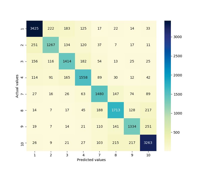
The figure 4.1, 4.1a is a confusion matrix for LSTM using porter stemming and
4.1b is a confusion matrix for GRU using porter stemming. When we observe the
true-positive values of LSTM and GRU, there is some contrast. we can observe that
LSTM has higher true-positive values for the class of sentiments 1, 4, 5 and 10 but
on the other side, GRU has higher true-positive values for the class of sentiments 2,
3, 8, and 9.
If we look at false-positive and false-negative values, we can observe that LSTM
has less false-positive values, whereas GRU has less false-negative values. It can
be argued that LSTM in combination with porter stemming predicts border values
more accurately. We can observe that there is very less difference between overall
predicted values of LSTM and GRU. We can say that GRU predicts better when
compare to LSTM for every class.
(a) LSTM-PS (b) GRU-PS
Figure 4.1: Confusion matrix heat map for Porter Stemming
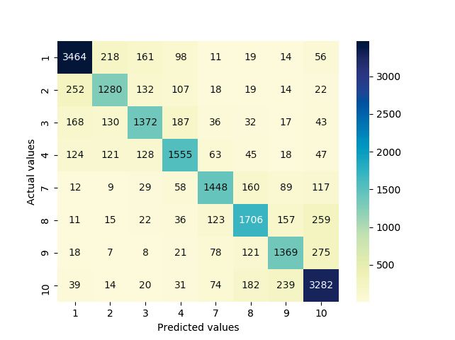
In the figure 4.2, 4.2a and 4.2b are confusion matrix for LSTM and GRU when
we use stop words pre-processing technique. Overall GRU has more true positive
values than LSTM. This implies GRU works better with stop words than LSTM.
In the figure 4.3, 4.3a and 4.3b are confusion matrix for LSTM and GRU when
we use basic pre-processing technique. When we compare the two matrices, there is
not much of a difference in the overall values of true positive, false negative and false
positive values. LSTM predicts better for class of sentiment 1 and 10 but overall
both LSTM and GRU performed similarly.
If we look at the test data accuracy in table 4.2, there is a very small difference4.2. Experiment 2 21
(a) LSTM-SW (b) GRU-SW
Figure 4.2: Confusion matrix heat map for Stop Words
(a) LSTM-B (b) GRU-B
Figure 4.3: Confusion matrix heat map for Basic
between the accuracies of LSTM and GRU. Hence, we use another method to compare
these two algorithms. We compared the learning rate for both LSTM and GRU to
find out which algorithm has higher learning rate.
To compare the learning rate, we selected accuracy graph of LSTM and GRU
with basic pre-processing shown in the figure 4.4. The reason for selecting basic
pre-processing is because the accuracy is quite similar for both LSTM and GRU.
Moreover, earlier we have seen LSTM and GRU performed similarly when we com-
pared confusion matrices for basic pre-processing.
In the figure 4.4, 4.4a and 4.4b is a line graph that visualizes the accuracy gained
for each epoch on training and validation data for 200 epochs. If we look at the struc-
ture of the curve, GRU attains higher accuracy before LSTM. Hence, this indicates
GRU has higher learning rate than LSTM.
The table 4.2 summarizes the results for all the six models. When we compare
the training time of these models with models addressed in section 4.1, there is a22 Chapter 4. Results and Analysis
(a) LSTM-B (b) GRU-B
Figure 4.4: Accuracy line graph for Basic
significant drop in training time for both LSTM and GRU models when we combine
them with CNN. The training time of LSTM is dropped by approximately 6 times,
whereas training time for GRU is dropped by approximately 14 times. Hence, this
shows there is a major improvement in performance when we couple the convolutional
layer with LSTM and GRU.
When we examine the maximum accuracy achieved on training data for LSTM
and GRU, we can see that LSTM has slightly higher accuracy than GRU. We can
argue that LSTM fits well for training data which is not essential. GRU predicts
slightly better than LSTM, this can be implied when we compare the maximum
accuracy achieved on validation data. The maximum accuracy of GRU on validation
data is equal or slightly higher for all the three pre-processing techniques (PS, SW,
B) when compared to LSTM.
Max
Time per Max
S. Validation Test data
Model Pre-processing Epochs Training
No. test Accuracy
(Average) accuracy
Accuracy
1 LSTM Porter Stemming(PS) 8.37 min 95.58 77.70 77.55
2 LSTM Stop Word(SW) 7.98 min 95.95 77.22 77.035
3 LSTM Basic(B) 8.13 min 95.88 77.56 77.38
4 GRU Porter Stemming(PS) 18.20 min 95.01 77.87 77.26
5 GRU Stop Word(SW) 17.51 min 94.35 77.39 77.53
6 GRU Basic(B) 17.33 min 94.96 77.56 77.27
Table 4.2: Experiment 2 Summary4.3. Experiment 3 23
4.3 Experiment 3
The tests addressed in this experiment are identical to experiment 2, the only differ-
ence is we increased the number of epochs to 500. The motive behind performing this
experiment is to check how much accuracy can be gained when we train the model
for a longer period. This is important for justifying how much we need to train the
model to achieve reasonable accuracy with the minimal computational cost.
When we compare the results in table 4.3 and table 4.2, there is a rise in max-
imum accuracy on training data. This could lead to overfitting as we can observe
a decline of accuracy for training data. There is a small increase in maximum ac-
curacy on validation data but the difference is not significant enough to justify the
computational cost.
Max
S. Max Training Validation Test data
Model Pre-processing
No. accuracy test Accuracy
Accuracy
1 LSTM Porter Stemming 97.47 78.11 77.59
2 LSTM Stop Word 97.53 77.23 76.98
3 LSTM Basic 97.08 77.63 77.23
4 GRU Porter Stemming 96.90 78.04 20.20
5 GRU Stop Word 95.01 77.46 76.6
6 GRU Basic 96.70 77.66 76.88
Table 4.3: Experiment 3 Summary
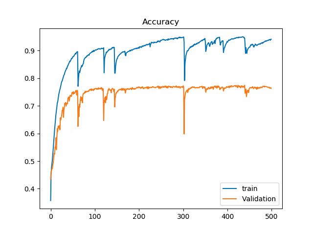
When we train a model for a longer time, the final model’s accuracy may drop
to the extent that it becomes useless. This can be observed in the figure 4.5, 4.5a
show there is fluctuation in the accuracy after 400 epochs. During the test, one of
the model’s accuracy falls to 20% and was never recovered, this can be seen in 4.5b.
After analyzing the results we can say that GRU performs slightly better than
LSTM, hence this answers the research question.24 Chapter 4. Results and Analysis
(a) LSTM-SW (b) GRU-PS
Figure 4.5: Accuracy line graph for BasicChapter 5
Discussion
After looking at the test results, we could say that both LSTM and GRU irrespective
of pre-processing techniques used achieved the accuracy of 77%. Hence, both LSTM
and GRU are similar in terms of accuracy. This deduction may be incorrect as several
other things needed to be considered.
Firstly, 77% accuracy may seem ok if we compare it with the general mark of
90% and above. Here we need to consider the number of classes for classification.
As for binary classification, the minimum accuracy baseline is 50% (100/2) or above.
Whereas in our model, there are eight different class labels. Hence, the baseline
would be 12.5% (100/12). When we compare 77% with 12.5% baseline the resultant
accuracy is quite good.
The dataset also plays a significant role in determining features of the mode. As
we see in the figure 3.1, the class label 1 and 10 have nearly double the number of
reviews than any other class label. Moreover, other class labels are also not balanced.
This imbalance in class labels may make models more sensitive to some classes than
others.
Similarly, there is also an disproportion in test dataset as we can see in the
table 5.1. This may have a significant impact on the overall accuracy of the model
on the test dataset. After a detailed analysis in the section 4.2, we could say that
GRU has performed better in predicting all classes for every pre-processing technique.
Hence, this answers the research question.
Class labels Count
1 4041
2 1844
3 1985
4 2101
7 1922
8 2329
9 1897
10 3881
Table 5.1: Test dataset
Another important aspect is the computational cost. After coupling LSTM and
GRU with the convolutional neural network, we were able to reduce the training time
for each epoch significantly. Even though we can still observe that GRU takes double
2526 Chapter 5. Discussion
the time for training when compared to LSTM. Hence we conclude that LSTM is
computationally cheaper than GRU.
One thing that we have to keep in mind is that the data which is used in training
and testing the models are generated by humans. The class labels are extracted
from the ratings given with the reviews. There may be several occurrences like two
different reviews may convey the same sentiment but have a distinct rating and
vice-versa.Chapter 6
Conclusions and Future Work
In this dissertation, we tried to compare the prediction accuracies of LSTM and
GRU for multiclass classification of text reviews given for movies. During the time
of testing, we found out that both LSTM and GRU were computationally expensive.
We coupled LSTM and GRU with CNN, which reduced the training time significantly.
After in-depth analysis, we found out that GRU is slightly better than LSTM and
also computationally expansive.
For future work, we can conduct the same experiments using properly balanced
dataset and study how this effect the models. An in-depth study can be conducted
on how CNN layer increased the performance of LSTM and GRU.
27References
[1] Bag of words meets bags of popcorn.
[2] Machine learning textbook.
[3] Understanding LSTM networks – colah’s blog.
[4] Cs 230 - recurrent neural networks cheatsheet. https://stanford.edu/
~shervine/teaching/cs-230/cheatsheet-recurrent-neural-networks, 06
2020. (Accessed on 04/06/2020).
[5] Shoiab Ahmed and Ajit Danti. A novel approach for sentimental analysis and
opinion mining based on SentiWordNet using web data. In 2015 International
Conference on Trends in Automation, Communications and Computing Tech-
nology (I-TACT-15), pages 1–5.
[6] Y. Bengio, P. Simard, and P. Frasconi. Learning long-term dependencies with
gradient descent is difficult. IEEE Transactions on Neural Networks, 5(2):157–
166, 1994.
[7] Shamim Biswas, Ekamber Chadda, and Faiyaz Ahmad. Sentiment analysis with
gated recurrent units.
[8] Jason Brownlee. Sequence classification with LSTM recurrent neural networks
in python with keras.
[9] Jose Camacho-Collados and Mohammad Taher Pilehvar. On the role of text
preprocessing in neural network architectures: An evaluation study on text cat-
egorization and sentiment analysis.
[10] François Chollet et al. Keras. https://keras.io, 2015.
[11] Junyoung Chung, Caglar Gulcehre, KyungHyun Cho, and Y. Bengio. Empirical
evaluation of gated recurrent neural networks on sequence modeling. 12 2014.
[12] Ian Goodfellow, Yoshua Bengio, and Aaron Courville. Deep Learning. MIT
Press, 2016. http://www.deeplearningbook.org.
[13] Sepp Hochreiter and Jürgen Schmidhuber. Long short-term memory. Neural
computation, 9:1735–80, 12 1997.
[14] IMDB. Parasite (2019) - parasite (2019) - user reviews - imdb. https://www.
imdb.com/title/tt6751668/reviews, 04 2020. (Accessed on 04/06/2020).
2930 References
[15] Import.io. What is data visualization and why is it important?
[16] Yoon Kim. Convolutional neural networks for sentence classification.
[17] Y. Lecun, L. Bottou, Y. Bengio, and P. Haffner. Gradient-based learning applied
to document recognition. 86(11):2278–2324.
[18] Li-xia Luo. Network text sentiment analysis method combining LDA text rep-
resentation and GRU-CNN. 23(3):405–412.
[19] Andrew L. Maas, Raymond E. Daly, Peter T. Pham, Dan Huang, Andrew Y.
Ng, and Christopher Potts. Learning word vectors for sentiment analysis. In
Proceedings of the 49th Annual Meeting of the Association for Computational
Linguistics: Human Language Technologies, pages 142–150, Portland, Oregon,
USA, June 2011. Association for Computational Linguistics.
[20] K. Mouthami, K. N. Devi, and V. M. Bhaskaran. Sentiment analysis and clas-
sification based on textual reviews. In 2013 International Conference on Infor-
mation Communication and Embedded Systems (ICICES), pages 271–276, 2013.
[21] Hadi Pouransari and Saman Ghili. Deep learning for sentiment analysis of movie
reviews.
[22] David Rumelhart, Geoffrey Hinton, and Ronald Williams. Learning representa-
tions by back propagating errors. Nature, 323:533–536, 10 1986.
[23] V. Srividhya and R. Anitha. Evaluating preprocessing techniques in text cate-
gorization. 47(11):49–51.
[24] W. F. Tichy. Should computer scientists experiment more? Computer, 31(5):32–
40, 1998.
[25] Jin Wang, Liang-Chih Yu, K. Robert Lai, and Xuejie Zhang. Dimensional
sentiment analysis using a regional CNN-LSTM model. In Proceedings of the
54th Annual Meeting of the Association for Computational Linguistics (Volume
2: Short Papers), pages 225–230.
[26] Alec Yenter and Abhishek Verma. Deep CNN-LSTM with combined kernels
from multiple branches for IMDb review sentiment analysis. In 2017 IEEE 8th
Annual Ubiquitous Computing, Electronics and Mobile Communication Confer-
ence (UEMCON), pages 540–546.
[27] Alec Yenter and Abhishek Verma. Deep CNN-LSTM with combined kernels
from multiple branches for IMDb review sentiment analysis. In 2017 IEEE 8th
Annual Ubiquitous Computing, Electronics and Mobile Communication Confer-
ence (UEMCON), pages 540–546.Appendix A
Supplemental Information
(a) LSTM-PS (b) GRU-PS
Figure A.1: Accuracy Line graphs for Porter Stemming
(a) LSTM-SW (b) GRU-SW
Figure A.2: Accuracy Line graphs for Stop words
3132 Appendix A. Supplemental Information
(a) LSTM-PS (b) LSTM-B
(c) GRU-SW (d) GRU-B
Figure A.3: Accuracy Line graphs for 500 EpochsFaculty of Computing, Blekinge Institute of Technology, 371 79 Karlskrona, Sweden
You can also read