Clash of the Titans: MapReduce vs. Spark for Large Scale Data Analytics
←
→
Page content transcription
If your browser does not render page correctly, please read the page content below
Clash of the Titans: MapReduce vs. Spark for Large Scale
                       Data Analytics

           Juwei Shi‡ , Yunjie Qiu† , Umar Farooq Minhas§ , Limei Jiao† , Chen Wang♯ , Berthold
                                                                     ∗
                                       Reinwald§ , and Fatma Özcan§
                                 †
                                   IBM Research - China § IBM Almaden Research Center
                 ‡
                     DEKE, MOE and School of Information, Renmin University of China ♯ Tsinghua University

ABSTRACT                                                                           are: MapReduce [7] and Spark [19]. These systems provide sim-
MapReduce and Spark are two very popular open source cluster                       ple APIs, and hide the complexity of parallel task execution and
computing frameworks for large scale data analytics. These frame-                  fault-tolerance from the user.
works hide the complexity of task parallelism and fault-tolerance,
by exposing a simple programming API to users. In this paper,                      1.1    Cluster Computing Architectures
we evaluate the major architectural components in MapReduce and                       MapReduce is one of the earliest and best known commodity
Spark frameworks including: shuffle, execution model, and caching,                 cluster frameworks. MapReduce follows the functional program-
by using a set of important analytic workloads. To conduct a de-                   ming model [8], and performs explicit synchronization across com-
tailed analysis, we developed two profiling tools: (1) We corre-                   putational stages. MapReduce exposes a simple programming API
late the task execution plan with the resource utilization for both                in terms of map() and reduce() functions. Apache Hadoop [1]
MapReduce and Spark, and visually present this correlation; (2)                    is a widely used open source implementation of MapReduce.
We provide a break-down of the task execution time for in-depth                       The simplicity of MapReduce is attractive for users, but the frame-
analysis. Through detailed experiments, we quantify the perfor-                    work has several limitations. Applications such as machine learn-
mance differences between MapReduce and Spark. Furthermore,                        ing and graph analytics iteratively process the data, which means
we attribute these performance differences to different components                 multiple rounds of computation are performed on the same data. In
which are architected differently in the two frameworks. We fur-                   MapReduce, every job reads its input data, processes it, and then
ther expose the source of these performance differences by using                   writes it back to HDFS. For the next job to consume the output of a
a set of micro-benchmark experiments. Overall, our experiments                     previously run job, it has to repeat the read, process, and write cy-
show that Spark is about 2.5x, 5x, and 5x faster than MapReduce,                   cle. For iterative algorithms, which want to read once, and iterate
for Word Count, k-means, and PageRank, respectively. The main                      over the data many times, the MapReduce model poses a signifi-
causes of these speedups are the efficiency of the hash-based aggre-               cant overhead. To overcome the above limitations of MapReduce,
gation component for combine, as well as reduced CPU and disk                      Spark [19] uses Resilient Distributed Datasets (RDDs) [19] which
overheads due to RDD caching in Spark. An exception to this is                     implement in-memory data structures used to cache intermediate
the Sort workload, for which MapReduce is 2x faster than Spark.                    data across a set of nodes. Since RDDs can be kept in memory,
We show that MapReduce’s execution model is more efficient for                     algorithms can iterate over RDD data many times very efficiently.
shuffling data than Spark, thus making Sort run faster on MapRe-                      Although MapReduce is designed for batch jobs, it is widely
duce.                                                                              used for iterative jobs. On the other hand, Spark has been de-
                                                                                   signed mainly for iterative jobs, but it is also used for batch jobs.
                                                                                   This is because the new big data architecture brings multiple frame-
1. INTRODUCTION                                                                    works together working on the same data, which is already stored
   In the past decade, open source analytic software running on                    in HDFS [17]. We choose to compare these two frameworks due
commodity hardware made it easier to run jobs which previously                     to their wide spread adoption in big data analytics. All the major
used to be complex and tedious to run. Examples include: text                      Hadoop vendors such as IBM, Cloudera, Hortonworks, and MapR
analytics, log analytics, and SQL like query processing, running                   bundle both MapReduce and Spark with their Hadoop distributions.
at a very large scale. The two most popular open source frame-
works for such large scale data processing on commodity hardware                   1.2    Key Architectural Components
∗This work has been done while Juwei Shi and Chen Wang were                           In this paper, we conduct a detailed analysis to understand how
Research Staff Members at IBM Research-China.                                      Spark and MapReduce process batch and iterative jobs, and what
                                                                                   architectural components play a key role for each type of job. In
                                                                                   particular, we (1) explain the behavior of a set of important ana-
This work is licensed under the Creative Commons Attribution-
NonCommercial-NoDerivs 3.0 Unported License. To view a copy of this li-            lytic workloads which are typically run on MapReduce and Spark,
cense, visit http://creativecommons.org/licenses/by-nc-nd/3.0/. Obtain per-        (2) quantify the performance differences between the two frame-
mission prior to any use beyond those covered by the license. Contact              works, (3) attribute these performance differences to the differences
copyright holder by emailing info@vldb.org. Articles from this volume              in their architectural components.
were invited to present their results at the 42nd International Conference on         We identify the following three architectural components and
Very Large Data Bases, September 5th - September 9th 2016, New Delhi,              evaluate them through detailed experiments. Studying these com-
India.
Proceedings of the VLDB Endowment, Vol. 8, No. 13                                  ponents covers the majority of architectural differences between
Copyright 2015 VLDB Endowment 2150-8097/15/09.                                     MapReduce and Spark.

                                                                                2110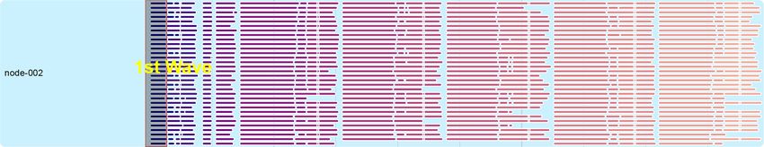
Shuffle: The shuffle component is responsible for exchanging in-            differences in their shuffle component. (3) Through a detailed anal-
termediate data between two computational stages 1 . For example,           ysis of the execution plan with the corresponding resource utiliza-
in the case of MapReduce, data is shuffled between the map stage            tion, we attribute performance differences to differences in major
and the reduce stage for bulk synchronization. The shuffle compo-           architectural components for the two frameworks. (4) We conduct
nent often affects the scalability of a framework. Very frequently,         micro-benchmark experiments to further explain non-trivial obser-
a sort operation is executed during the shuffle stage. An external          vations regarding RDD caching.
sorting algorithm, such as merge sort, is often required to handle             The rest of the paper is organized as follows. We provide the
very large data that does not fit in main memory. Furthermore, ag-          workload description in Section 2. In Section 3, we present our
gregation and combine are often performed during a shuffle.                 experimental results along with a detailed analysis. Finally, we
Execution Model: The execution model component determines                   present a discussion and summary of our findings in Section 4.
how user defined functions are translated into a physical execution
plan. The execution model often affects the resource utilization            2.      WORKLOAD DESCRIPTION
for parallel task execution. In particular, we are interested in (1)           In this section, we identify a set of important analytic workloads
parallelism among tasks, (2) overlap of computational stages, and           including Word Count (WC), Sort, k-means, linear regression (LR),
(3) data pipelining among computational stages.                             and PageRank.
Caching: The caching component allows reuse of intermediate
data across multiple stages. Effective caching speeds up iterative                      Table 1: Characteristics of Selected Workloads
algorithms at the cost of additional space in memory or on disk.                                                Word    Sort   K-Means    Page-
                                                                                                                Count          (LR)       Rank
In this study, we evaluate the effectiveness of caching available                                               √       √
                                                                                                    One Pass                   √          √
at different levels including OS buffer cache, HDFS caching [3],                   Type             Iterative           √
Tachyon [11], and RDD caching.                                                                      High                                  √
   For our experiments, we use five workloads including Word                       Shuffle Sel.     Medium      √              √
                                                                                                    Low                 √
Count, Sort, k-means, linear regression, and PageRank. We choose                                    High
these workloads because collectively they cover the important char-                                                                       √
                                                                                   Job/Iter. Sel.   Medium      √              √
acteristics of analytic workloads which are typically run on MapRe-                                 Low
duce and Spark, and they stress the key architectural components
we are interested in, and hence are important to study. Word Count             As shown in Table 1, the selected workloads collectively cover
is used to evaluate the aggregation component because the size of           the characteristics of typical batch and iterative analytic applica-
intermediate data can be significantly reduced by the map side com-         tions run on MapReduce and Spark. We evaluate both one-pass
biner. Sort is used to evaluate the external sort, data transfer, and       and iterative jobs. For each type of job, we cover different shuf-
the overlap between map and reduce stages because the size of in-           fle selectivity (i.e., the ratio of the map output size to the job input
termediate data is large for sort. K-Means and PageRank are used            size, which represents the amount of disk and network I/O for a
to evaluate the effectiveness of caching since they are both iterative      shuffle), job selectivity (i.e., the ratio of the reduce output size to
algorithms. We believe that the conclusions which we draw from              the job input size, which represents the amount of HDFS writes),
these workloads running on MapReduce and Spark can be gener-                and iteration selectivity (i.e., the ratio of the output size to the input
alized to other workloads with similar characteristics, and thus are        size for each iteration, which represents the amount of intermedi-
valuable.                                                                   ate data exchanged across iterations). For each workload, given
                                                                            the I/O behavior represented by these selectivities, we evaluate its
1.3 Profiling Tools                                                         system behavior (e.g., CPU-bound, disk-bound, network-bound) to
   To help us quantify the differences in the above architectural           further identify the architectural differences between MapReduce
components between MapReduce and Spark, as well as the behav-               and Spark.
ior of a set of important analytic workloads on both frameworks,               Furthermore, we use these workloads to quantitatively evalu-
we developed the following tools for this study.                            ate different aspects of key architectural components including (1)
Execution Plan Visualization: To understand a physical exe-                 shuffle, (2) execution model, and (3) caching. As shown in Table 2,
cution plan, and the corresponding resource utilization behavior,           for the shuffle component, we evaluate the aggregation framework,
we correlate the task level execution plan with the resource utiliza-       external sort, and transfers of intermediate data. For the execu-
tion, and visually present this correlation, for both MapReduce and         tion model component, we evaluate how user defined functions are
Spark.                                                                      translated into to a physical execution plan, with a focus on task
Fine-grained Time Break-down: To understand where time goes                 parallelism, stage overlap, and data pipelining. For the caching
for the key components, we add timers to the Spark source code to           component, we evaluate the effectiveness of caching available at
provide the fine-grained execution time break-down. For MapRe-              different levels for caching both input and intermediate data. As
duce, we get this time break-down by extracting this information            explained in Section 1.2, the selected workloads collectively cover
from the task level logs available in the MapReduce framework.              all the characteristics required to evaluate these three components.

1.4 Contributions                                                           3.      EXPERIMENTS
   The key contributions of this paper are as follows. (1) We con-
duct experiments to thoroughly understand how MapReduce and                 3.1         Experimental Setup
Spark solve a set of important analytic workloads including both
batch and iterative jobs. (2) We dissect MapReduce and Spark                    3.1.1     Hardware Configuration
frameworks and collect statistics from detailed timers to quantify             Our Spark and MapReduce clusters are deployed on the same
1                                                                           hardware, with a total of four servers. Each node has 32 CPU cores
 For MapReduce, there are two stages: map and reduce. For Spark,
there may be many stages, which are built at shuffle dependencies.          at 2.9 GHz, 9 disk drives at 7.2k RPM with 1 TB each, and 190

                                                                         2111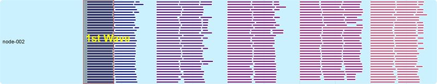
Metric Selection
Metric Selection
0 20 40 60 80 100 120 140 0 5 10 15 20 25 30 35 40 45
Time (sec) Time (sec)
100 CPU CPU
100
(%)
CPU_SYSTEM
(%)
80 CPU_SYSTEM 80
CPU_USER 60 60
40 CPU_USER
CPU_WIO 40
20 Time (sec) CPU_WIO 20 Time (sec)
0 20 40 60 80 100 120 140 0 5 10 15 20 25 30 35 40 45
0%
9%
MEMORY MEMORY
(GB)
MEM_CACHED 200
(GB)
MEM_CACHED 200
160 160
MEM_TOTAL 120 MEM_TOTAL 120
80 80
MEM_USED 40 MEM_USED
Time (sec) 40 Time (sec)
0 20 40 60 80 100 120 140 0 5 10 15 20 25 30 35 40 45
NETWORK NETWORK
(MB/s)
BYTES_IN
(MB/s)
100 BYTES_IN 100
80 80
BYTES_OUT 60 BYTES_OUT
40 60
20 40
Time (sec) 20 Time (sec)
0 20 40 60 80 100 120 140 0 5 10 15 20 25 30 35 40 45
DISK_IO DISK_IO
(MB/s)
sdb_READ
(MB/s)
100 sdb_READ 100
sdb_WRITE 80 80
60 sdb_WRITE 60
sdc_READ 40 40
20 sdc_READ
sdc_WRITE Time (sec) 20 Time (sec)
0 20 40 60 80 100 120 140 sdc_WRITE
0 5 10 15 20 25 30 35 40 45
100 DISK_USAGE DISK_USAGE
100
(%)
sdb_
(%)
80 sdb_ 80
sdc_ 60 60
40 sdc_
40
20 Time (sec) 20 Time (sec)
0 20 40 60 80 100 120 140 0 5 10 15 20 25 30 35 40 45
(a) MapReduce (b) Spark
Figure 1: The Execution Details of Word Count (40 GB)
Table 2: Key Architectural Components of Interest output; (2) For all workloads except Sort, we disable the overlap
Word Sort K-Means Page- between map and reduce stages. This overlap hides the network
Count (LR) Rank overhead by overlapping computation and network transfer. But it
√ √ √
Aggregation √ comes at a cost of reduction in map parallelism, and the network
Shuffle External sort √ √
Data transfer overhead is not a bottleneck for any workload except Sort; (3) For
√ √ √ √
Task parallelism √
Sort, we set the number of reduce tasks to 60 to overlap the shuffle
Execution Stage overlap √ stage (network-bound) with the map stage (without network over-
Data pipelining √ √
Input
head), and for other workloads, we set the number of reduce tasks
√ to 120; (4) We set the number of parallel copiers per task to 2 to
Caching Intermediate data
reduce the context switching overhead [16]; (5) We set the map
output buffer to 550 MB to avoid additional spills for sorting the
GB of physical memory. In aggregate, our four node cluster has map output; (6) For Sort, we set the reduce input buffer to 75% of
128 CPU cores, 760 GB RAM, and 36 TB locally attached storage. the JVM heap size to reduce the disk overhead caused by spills.
The hard disks deliver an aggregate bandwidth of about 125 GB/sec
Spark: We use Spark version 1.3.0 running in the standalone
for reads and 45 GB/sec for writes across all nodes, as measured
mode on HDFS 2.4.0. We also use 8 disks for storing Spark in-
using dd. Nodes are connected using a 1 Gbps Ethernet switch.
termediate data. For each node, we run 8 Spark workers where
Each node runs 64-bit Red Hat Enterprise Linux 6.4 (kernel version
each worker is configured with 4 threads (i.e., one thread per CPU
2.6.32).
core). We also tested other configurations. We found that when we
As a comparison, hardware specifications of our physical cluster
run 1 worker with 32 threads, the CPU utilization is significantly
are roughly equivalent to a cluster with about 100 virtual machines
reduced. For example, under this configuration, the CPU utilization
(VMs) (e.g., m3.medium on AWS2 ). Our hardware setup is suitable
decreases to 33% and 25%, for Word Count and the first iteration of
for evaluating various scalability bottlenecks in Spark and MapRe-
k-means, respectively. This may be caused by the synchronization
duce frameworks. For example, we have enough physical cores in
overhead of memory allocation for multi-threaded tasks. However,
the system to run many concurrent tasks and thus expose any syn-
CPU can be 100% utilized for all the CPU-bound workloads when
chronization overheads. However, experiments which may need a
using 8 workers with 4 threads each. Thus, we use this setting for
large number of servers (e.g., evaluating the scalability of master
our experiments. We set the JVM heap size to 16 GB for both the
nodes) are out of the scope of this paper.
Spark driver and the executors. Furthermore, we tune the following
parameters for Spark: (1) We use Snappy to compress the interme-
3.1.2 Software Configuration
diate results during a shuffle; (2) For Sort with 500 GB input, we set
Both MapReduce and Spark are deployed on Java 1.7.0. the number of tasks for shuffle reads to 2000. For other workloads,
Hadoop: We use Hadoop version 2.4.0 to run MapReduce on this parameter is set to 120.
YARN [17]. We use 8 disks to store intermediate data for MapRe-
duce and for storing HDFS data as well. We configure HDFS with 3.1.3 Profiling tools
128 MB block size and a replication factor of 3. We configure In this section, we present the visualization and profiling tools
Hadoop to run 32 containers per node (i.e., one per CPU core). To which we have developed to perform an in-depth analysis of the
better control the degree of parallelism for jobs, we enable CGroups selected workloads running on Spark and MapReduce.
in YARN and also enable CPU-Scheduling 3 . The default JVM
heap size is set to 3 GB per task. We tune the following parameters Execution Plan Visualization: To understand parallel execution
to optimize performance: (1) We use Snappy compression for map behavior, we visualize task level execution plans for both MapRe-
duce and Spark. First, we extract the execution time of tasks from
2
http://aws.amazon.com/ec2/instance-types/ job history of MapReduce and Spark. In order to create a compact
3
https://www.kernel.org/doc/Documentation/cgroups/cgroups.txt view to show parallelism among tasks, we group tasks to horizontal
2112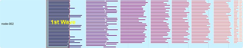
Table 3: Overall Results: Word Count Table 4: Time Break-down of Map Tasks for Word Count
Platform Spark MR Spark MR Spark MR Platform Load Read Map Combine Serialization Compression
Input size (GB) 1 1 40 40 200 200 (sec) (sec) (sec) (sec) (sec) &write (sec)
Number of map tasks 9 9 360 360 1800 1800 Spark 0.1 2.6 1.8 2.3 2.6 0.1
Number of reduce tasks 8 8 120 120 120 120 MapReduce 6.2 12.6 14.3 5.0
Job time (Sec) 30 64 70 180 232 630
Median time of map tasks (Sec) 6 34 9 40 9 40
Median time of reduce tasks (Sec) 4 4 8 15 33 50
Map Output on disk (GB) 0.03 0.015 1.15 0.7 5.8 3.5
amount of intermediate data is similar. We believe that this dif-
ference is due to the differences in the aggregation component. We
evaluate this observation further in Section 3.2.3 below.
For the reduce stage, the execution time is very similar in Spark
lines. We deploy Ganglia [13] over the cluster, and persist Round-
and MapReduce because the reduce stage is network-bound and the
Robin Database [5] to MySQL database periodically. Finally, we
amount of data to shuffle is similar in both cases.
correlate the system resource utilization (CPU, memory, disk, and
network) with the execution plan of tasks using a time line view. 3.2.2 Execution Details
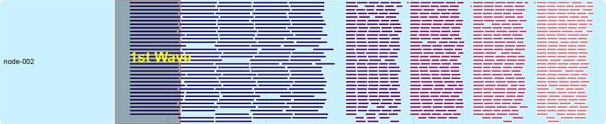
Figure 1 is an example of such an execution plan visualization.
Figure 1 shows the detailed execution plan for WC with 40 GB
At the very top, we present a visualization of the physical execu-
input. Our deployment of both MapReduce and Spark can exe-
tion plan where each task is represented as an horizontal line. The
cute 128 tasks in parallel, and each task processes 128 MB of data.
length of this line is proportional to the actual execution time of a
Therefore, it takes three waves of map tasks (shown in blue in Fig-
task. Tasks belonging to different stages are represented in differ-
ure 1) to process the 40 GB input. As we show the execution time
ent colors. The physical execution plan can then be visually corre-
when the first task starts on the cluster, there may be some initial-
lated with the CPU, memory, network, and disk resources, which
ization lag on worker nodes (e.g., 0 to 4 seconds in Figure 1 (b)).
are also presented in Figure 1. In the resource utilization graphs,
x-axis presents the elapsed time in seconds, and is correlated with Map Stage: We observe that in Spark, the map stage is disk-bound
the horizontal axis of the physical execution plan. Moreover, we while in MapReduce it is CPU-bound. As each task processes the
break down reduce tasks for MapReduce to three sub-stages: copy, same amount of data (i.e., 128 MB), this indicates that Spark takes
sort, and reduce. For each batch of simultaneously running task less CPU time than MapReduce in the map stage. This is consistent
(i.e., wave), we can read directly down to correlate resources with with the 3x speed-up shown in Table 3.
the processing that occurs during that wave. Reduce Stage: The network resource utilization in Figure 1 shows
This tool can show: (1) parallelism of tasks (i.e., waves), e.g., that the reduce stage is network-bound for both Spark and MapRe-
the first wave is marked in Figure 1 (a), (2) the overlap of stages, duce. However, the reduce stage is not a bottleneck for WC because
e.g., the overlap between map and reduce stages is shown in Fig- (1) most of the computation is done during the map side combine,
ure 2 (b), (3) skewness of tasks, e.g., the skewness of map tasks and (2) the shuffle selectivity is low (< 2%), which means that
is shown in Figure 3 (b), and (4) the resource usage behavior for reduce tasks have less data to process.
each stage, e.g., we can see that the map stage is CPU-bound in
Figure 3 (a). Note that the goal of our visualization tool is to help 3.2.3 Breakdown for the Map Stage
a user analyze details of the physical execution plan, and the corre- In order to explain the 3x performance difference during the map
sponding resource utilization, in order to gain deeper insights into stage, we present the execution time break-down for map tasks in
a workload’s behavior. both Spark and MapReduce in Table 4. The reported execution
times are an average over 360 map tasks with 40 GB input to WC.
Fine-grained Time Break-down: To understand where time goes
First, MapReduce is much slower than Spark in task initialization.
for the shuffle component, we provide the fine-grained execution
Second, Spark is about 2.9x faster than MapReduce in input read
time break-down for selected tasks. For Spark, we use System.na-
and map operations. Last, Spark is about 6.2x faster than MapRe-
noTime() to add timers to each sub-stage, and aggregate the time
duce in the combine stage. This is because the hash-based combine
after a task finishes. In particular, we add timers to the following
is more efficient than the sort-based combine for WC. Spark has
components: (1) compute() method for RDD transformation, (2)
lower complexity in its in-memory collection and combine compo-
ShuffleWriter for combine, and (3) BlockObjectWriter for
nents, and thus is faster than MapReduce.
serialization, compression, and shuffle writes. For MapReduce, we
use the task logs to provide the execution time break-down. We find 3.2.4 Summary of Insights
that such detailed break-downs are sufficient to quantify differences
For WC and similar workloads such as descriptive statistics, the
in the shuffle components of MapReduce and Spark.
shuffle selectivity can be significantly reduced by using a map side
combiner. For this type of workloads, hash-based aggregation in
3.2 Word Count Spark is more efficient than sort-based aggregation in MapReduce
We use Word Count (WC) to evaluate the aggregation compo- due to the complexity differences in its in-memory collection and
nent for both MapReduce and Spark. For these experiments, we combine components.
use the example WC program included with both MapReduce and
Spark, and we use Hadoop’s random text writer to generate input. 3.3 Sort
For experiments with Sort, we use TeraSort [15] for MapRe-
3.2.1 Overall Result duce, and implement Sort using sortByKey() for Spark. We
use gensort 4 to generate the input for both.
Table 3 presents the overall results for WC for various input
We use experiments with Sort to analyze the architecture of the
sizes, for both Spark and MapReduce. Spark is about 2.1x, 2.6x,
shuffle component in MapReduce and Spark. The shuffle compo-
and 2.7x faster than MapReduce for 1 GB, 40 GB, and 200 GB
nent is used by Sort to get a total order on the input and is a bottle-
input, respectively.
neck for this workload.
Interestingly, Spark is about 3x faster than MapReduce in the
4
map stage. For both frameworks, the application logic and the http://www.ordinal.com/gensort.html
2113Metric Selection
Metric Selection
0 20 40 60 80 100 120 140 160 180
Time (sec) 0 30 60 90 120 150 180 210 240 270
100 CPU CPU
Time (sec)
(%)
CPU_SYSTEM 100
(%)
80 CPU_SYSTEM
60 80
CPU_USER 60
40 CPU_USER
CPU_WIO 20 40
Time (sec) CPU_WIO 20 Time (sec)
0 20 40 60 80 100 120 140 160 180
0 30 60 90 120 150 180 210 240 270
MEMORY MEMORY
(GB)
MEM_CACHED 200
(GB)
160 MEM_CACHED 200
MEM_TOTAL 120 160
80 MEM_TOTAL 120
MEM_USED 40 80
Time (sec) MEM_USED 40 Time (sec)
0 20 40 60 80 100 120 140 160 180
0 30 60 90 120 150 180 210 240 270
NETWORK NETWORK
(MB/s)
BYTES_IN 100
(MB/s)
80 BYTES_IN 100
BYTES_OUT 60 80
40
BYTES_OUT 60
20 40
Time (sec) 20 Time (sec)
0 20 40 60 80 100 120 140 160 180
0 30 60 90 120 150 180 210 240 270
DISK_IO DISK_IO
(MB/s)
sdb_READ 100
(MB/s)
80 sdb_READ 100
sdb_WRITE 60 80
sdb_WRITE 60
sdc_READ 40
20 sdc_READ 40
sdc_WRITE Time (sec) 20
sdc_WRITE Time (sec)
0 20 40 60 80 100 120 140 160 180
0 30 60 90 120 150 180 210 240 270
100 DISK_USAGE DISK_USAGE
(%)
sdb_ 100
(%)
80 sdb_
60 80
sdc_ 60
40 sdc_
20 40
Time (sec) 20 Time (sec)
0 20 40 60 80 100 120 140 160 180
0 30 60 90 120 150 180 210 240 270
(a) MapReduce (b) Spark
Figure 2: The Execution Details of Sort (100 GB Input)
Table 5: Overall Results: Sort Table 6: Time Break-down of Map Tasks for Sort
Platform Load Read Map Combine Serialization Compression
Platform Spark MR Spark MR Spark MR (sec) (sec) (sec) (sec) (sec) &write (sec)
Input size (GB) 1 1 100 100 500 500 Spark-Hash 0.1 1.1 0.8 - 3.0 5.5
Number of map tasks 9 9 745 745 4000 4000 Spark-Sort 0.1 1.2 0.6 6.4 2.3 2.4
Number of reduce tasks 8 8 248 60 2000 60 MapReduce 6.6 10.5 4.1 2.0
Job time 32s 35s 4.8m 3.3m 44m 24m
Sampling stage time 3s 1s 1.1m 1s 5.2m 1s
Map stage time 7s 11s 1.0m 2.5m 12m 13.9m mentioned earlier, Spark scans the whole input file during sampling
Reduce stage time 11s 24s 2.5m 45s 26m 9.2m and is therefore disk-bound.
Map output on disk (GB) 0.63 0.44 62.9 41.3 317.0 227.2
Map Stage: As shown in Figure 2, both Spark and MapReduce are
CPU-bound in the map stage. Note that the second stage is the map
3.3.1 Overall Result stage for Spark. Even though Spark and MapReduce use different
Table 5 presents the overall results for Sort for 1 GB, 100 GB, shuffle frameworks, their map stages are bounded by map output
and 500 GB input, for both Spark and MapReduce. For 1 GB input, compression. Furthermore, for Spark, we observe that disk I/O is
Spark is faster than MapReduce because Spark has lower control significantly reduced in the map stage compared to the sampling
overhead (e.g., task load time) than MapReduce. MapReduce is stage, although its map stage also scans the whole input file. The
1.5x and 1.8x faster than Spark for 100 GB and 500 GB inputs, reduced disk I/O is a result of reading input file blocks cached in
respectively. Note that the results presented in [6] show that Spark the OS buffer during the sampling stage.
outperformed MapReduce in the Daytona Gray Sort benchmark. Reduce Stage: The reduce stage in both Spark and MapReduce
This difference is mainly because our cluster is connected using 1 uses external sort to get a total ordering on the shuffled map output.
Gbps Ethernet, as compared to a 10 Gbps Ethernet in [6], i.e., in MapReduce is 2.8x faster than Spark for this stage. As the execu-
our cluster configuration network can become a bottleneck for Sort tion plan for MapReduce in Figure 2 (a) shows, the main cause of
in Spark, as explained in Section 3.3.2 below. this speed-up is that the shuffle stage is overlapped with the map
From Table 5 we can see that for the sampling stage, MapReduce stage, which hides the network overhead. The current implemen-
is much faster than Spark because of the following reason: MapRe- tation of Spark does not support the overlap between shuffle write
duce reads a small portion of the input file (100, 000 records from and read stages. This is a notable architectural difference between
10 selected splits), while Spark scans the whole file. For the map MapReduce and Spark. Spark may want to support this overlap in
stage, Spark is 2.5x and 1.2x faster than MapReduce for 100 GB the future to improve performance. Last, note that the number of
and 500 GB input, respectively. For the reduce stage, MapReduce replicas in this experiment is set to 1 according to the sort bench-
is 3.3x and 2.8x faster than Spark for 100 GB and 500 GB input, mark [15], thus there is no network overhead for HDFS writes in
respectively. To better explain this difference, we present a detailed reduce tasks.
analysis of the execution plan in Section 3.3.2 and a break-down of When the input size increases from 100 GB to 500 GB, during
the execution time in Section 3.3.3 below. the map stage in Spark, there is significant CPU overhead for swap-
ping pages in OS buffer cache. However, for MapReduce, we ob-
3.3.2 Execution Details
serve much less system CPU overhead during the map stage. This
Figure 2 shows the detailed execution plan of 100 GB Sort for is the main reason that the map stage speed-up between Spark and
MapReduce and Spark along with the resource utilization graphs. MapReduce is reduced from 2.5x to 1.2x.
Sampling Stage: The sampling stage of MapReduce is performed
by a lightweight central program in less than 1 second, so it is not 3.3.3 Breakdown for the Map Stage
shown in the execution plan. Figure 2 (b) shows that during the Table 6 shows a break-down of the map task execution time for
initial part of execution (i.e., sampling stage) in Spark, the disk both MapReduce and Spark, with 100 GB input. A total of 745
utilization is quite high while the CPU utilization is low. As we map tasks are executed, and we present the average execution time.
2114We find that there are two stages where MapReduce is slower than Table 7: Overall Results: K-Means
Spark. First, the load time in MapReduce is much slower than that Platform Spark MR Spark MR Spark MR
in Spark. Second, the total times of (1) reading the input (Read), Input size (million records) 1 1 200 200 1000 1000
Iteration time 1st 13s 20s 1.6m 2.3m 8.4m 9.4m
and (2) for applying the map function on the input (Map), is higher Iteration time Subseq. 3s 20s 26s 2.3m 2.1m 10.6m
than Spark. The reasons why Spark performs better include: (1) Median map task time 1st 11s 19s 15s 46s 15s 46s
Spark reads part of the input from the OS buffer cache since its sam- Median reduce task time 1st 1s 1s 1s 1s 8s 1s
Median map task time Subseq. 2s 19s 4s 46s 4s 50s
pling stage scans the whole input file. On the other hand, MapRe- Median reduce task time Subseq. 1s 1s 1s 1s 3s 1s
duce only partially reads the input file during sampling thus OS Cached input data (GB) 0.2 - 41.0 - 204.9 -
buffer cache is not very effective during the map stage. (2) MapRe-
duce collects the map output in a map side buffer before flushing
it to disk, but Spark’s hash-based shuffle writer, writes each map optimization covers a large set of iterative machine learning algo-
output record directly to disk, which reduces latency. rithms such as linear regression, logistic regression, and support
vector machine. Therefore, the observations we draw from the re-
3.3.4 Comparison of Shuffle Components sults presented in this section for k-means are generally applicable
Since Sort is dominated by the shuffle stage, we evaluate differ- to the above mentioned algorithms.
ent shuffle frameworks including hash-based shuffle (Spark-Hash), As shown in Table 1, both the shuffle selectivity and the iteration
sort-based shuffle (Spark-Sort), and MapReduce. selectivity of k-means is low. Suppose there are N input records
First, we find that the execution time of the map stage increases to train K centroids, both map output (for each task) and job out-
as we increase the number of reduce tasks, for both Spark-Hash and put only have K records . Since K is often much smaller than N ,
Spark-Sort. This is because of the increased overhead for handling both the shuffle and iteration selectivities are very small. As shown
opened files and the commit operation of disk writes. As opposed to in Table 2, the training data can be cached in-memory for subse-
Spark, the number of reduce tasks has little effect on the execution quent iterations. This is common in machine learning algorithms.
time of the map stage for MapReduce. Therefore, we use k-means to evaluate the caching component.
The number of reduce tasks has no affect on the execution time
of Spark’s reduce stage. However, for MapReduce, the execution 3.4.1 Overall Result
time of the reduce stage increases as more reduce tasks are used Table 7 presents the overall results for k-means for various in-
because less map output can be copied in parallel with the map put sizes, for both Spark and MapReduce. For the first iteration,
stage as the number of reduce tasks increases. Spark is about 1.5x faster than MapReduce. For subsequent itera-
Second, we evaluate the impact of buffer sizes for both Spark tions, because of RDD caching, Spark is more than 5x faster than
and MapReduce. For both MapReduce and Spark, when the buffer MapReduce for all input sizes.
size increases, the reduced disk spills cannot lead to the reduction We compare the performance of various RDD caching options
in the execution time since disk I/O is not a bottleneck. However, (i.e., storage levels) available in Spark, and we find that the effec-
the increased buffer size may lead to slow-down in Spark due to the tiveness of all the persistence mechanisms is almost the same for
increased overhead for GC and page swapping in OS buffer cache. this workload. We explain the reason in Section 3.4.3.
Another interesting observation is that when there is no in-heap
3.3.5 Summary of Insights caching (i.e., for Spark without RDD caching and MapReduce), the
For Sort and similar workloads such as Nutch Indexing and disk I/O decreases from one iteration to the next iteration because
TFIDF [10], the shuffle selectivity is high. For this type of work- of the increased hit ratio of OS buffer cache for input from HDFS.
loads, we summarize our insights from Sort experiments as follows: However, this does not result in a reduction in the execution time.
(1) In MapReduce, the reduce stage is faster than Spark because We explain these observations in Section 3.4.4.
MapReduce can overlap the shuffle stage with the map stage, which
effectively hides the network overhead. (2) In Spark, the execution 3.4.2 Execution Details
time of the map stage increases as the number of reduce tasks in- Figure 3 shows the detailed execution plan for k-means with an
crease. This overhead is caused by and is proportional to the num- input of 200 million records for MapReduce and Spark. We present
ber of files opened simultaneously. (3) For both MapReduce and the first five iterations. Subsequent iterations exhibit similar char-
Spark, the reduction of disk spills during the shuffle stage may not acteristics.
lead to the speed-up since disk I/O is not a bottleneck. However, Map Stage: For both MapReduce and Spark, the map stage takes
for Spark, the increased buffer may lead to the slow-down because up more than 99% of the total execution time in each iteration and
of increased overhead for GC and OS page swapping. hence is the bottleneck. During the map stage, both MapReduce
and Spark scan the training data to update the cluster centroids.
3.4 Iterative Algorithms: K-Means and Lin- For MapReduce (Mahout k-means), it uses a map side hash table
ear Regression to combine the updated value of the centroid. For Spark, it uses
K-Means is a popular clustering algorithm which partitions N a map side combiner (implemented in reduceByKey()) to up-
observations into K clusters in which each observation belongs to date centroids. The shuffle selectivity is very small. For example,
the cluster with the nearest mean. We use the generator from Hi- with 200 million records, the selectivity is 0.00001 and 0.004, for
Bench [10] to generate training data for k-means. Each training MapReduce and Spark, respectively.
record (point) has 20 dimensions. We use Mahout [2] k-means for The map stage is CPU-bound for all iterations of both MapRe-
MapReduce, and the k-means program from the example package duce and Spark due to the low shuffle selectivity. Moreover, for
for Spark. We revised the Mahout code to use the same initial cen- MapReduce, we observe that the disk read overhead decreases from
troids and convergence condition for both MapReduce and Spark. one iteration to the next iteration. Since there is no in-heap caching
K-Means is representative of iterative machine learning algo- in MapReduce framework, it depends on OS buffer to cache the
rithms. For each iteration, it reads the training data to calculate training data. However, OS buffer cache does not result in exe-
updated parameters (i.e., centroids). This pattern for parameter cution time improvements, as we show later in Section 3.4.4. As
2115Metric Selection
Metric Selection
0 75 150 225 300 375 450 525 600 675 0 20 40 60 80 100 120 140 160 180
Time (sec) Time (sec)
100 CPU CPU
100
(%)
CPU_SYSTEM
(%)
80 CPU_SYSTEM 80
CPU_USER 60 60
40 CPU_USER
CPU_WIO 40
20 Time (sec) CPU_WIO 20 Time (sec)
0 75 150 225 300 375 450 525 600 675 0 20 40 60 80 100 120 140 160 180
0%
MEMORY MEMORY
(GB)
MEM_CACHED 200
(GB)
MEM_CACHED 200
160 160
MEM_TOTAL 120 MEM_TOTAL 120
80 80
MEM_USED 40 MEM_USED
Time (sec) 40 Time (sec)
0 75 150 225 300 375 450 525 600 675 0 20 40 60 80 100 120 140 160 180
NETWORK NETWORK
(MB/s)
BYTES_IN
(MB/s)
100 BYTES_IN 100
80 80
BYTES_OUT 60 BYTES_OUT
40 60
20 40
Time (sec) 20 Time (sec)
0 75 150 225 300 375 450 525 600 675 0 20 40 60 80 100 120 140 160 180
DISK_IO DISK_IO
(MB/s)
sdb_READ
(MB/s)
100 sdb_READ 100
sdb_WRITE 80 80
60 sdb_WRITE 60
sdc_READ 40 40
20 sdc_READ
sdc_WRITE Time (sec) 20 Time (sec)
0 75 150 225 300 375 450 525 600 675 sdc_WRITE
0 20 40 60 80 100 120 140 160 180
100 DISK_USAGE DISK_USAGE
100
(%)
sdb_
(%)
80 sdb_ 80
sdc_ 60 60
40 sdc_
40
20 Time (sec) 20 Time (sec)
0 75 150 225 300 375 450 525 600 675 0 20 40 60 80 100 120 140 160 180
(a) MapReduce (b) Spark
Figure 3: The Execution Details of K-Means (200 Million Records)
Table 8: The Impact of Storage Levels for K-Means Table 9: The Impact of Memory Constraints
Storage Levels Caches First Iter- Subsequent Storage Levels Fraction Persistence First Iter- Subsequent
Size ations Iterations ratio ations Iterations
NONE - 1.3m 1.2m MEMORY ONLY 0 0.0% 1.4m 1.2m
DISK ONLY 37.6 GB 1.5m 29s MEMORY ONLY 0.1 15.6% 1.5m 1.2m
DISK ONLY 2 37.6 GB 1.9m 27s MEMORY ONLY 0.2 40.7% 1.5m 1.0m
MEMORY ONLY 41.0 GB 1.5m 26s MEMORY ONLY 0.3 67.2% 1.6m 47s
MEMORY ONLY 2 41.0 GB 2.0m 25s MEMORY ONLY 0.4 98.9% 1.5m 33s
MEMORY ONLY SER 37.6 GB 1.5m 29s MEMORY ONLY 0.5 100% 1.6m 30s
MEMORY ONLY SER 2 37.6 GB 1.9m 28s MEMORY AND DISK 0 100% 1.5m 28s
MEMORY AND DISK 41.0 GB 1.5m 26s MEMORY AND DISK 0.1 100% 1.5m 30s
MEMORY AND DISK 2 41.0 GB 2.0m 25s MEMORY AND DISK 0.2 100% 1.6m 30s
MEMORY AND DISK SER 37.6 GB 1.5m 29s MEMORY AND DISK 0.3 100% 1.6m 28s
MEMORY AND DISK SER 2 37.6 GB 1.9m 27s MEMORY AND DISK 0.4 100% 1.5m 28s
OFF HEAP (Tachyon) 37.6 GB 1.5m 30s MEMORY AND DISK 0.5 100% 1.5m 28s
DISK ONLY - 100% 1.5m 29s
opposed to MapReduce, there is no disk read overhead in subse-
quent iterations for Spark, because the input is stored in memory RDD caching. We also evaluate the impact of memory constraints
as RDDs. Note that the 3.5x speed-up for subsequent iterations in on the effectiveness of RDD caching.
Spark cannot be fully attributed to the reduced disk I/O overhead. Impact of Storage Levels: The version of Spark we evaluate pro-
We explain this in Section 3.4.4. vides 11 storage levels including MEMORY ONLY, DISK ONLY,
Reduce Stage: Both MapReduce and Spark use a map-side com- MEMORY AND DISK, and Tachyon [11]. For memory only re-
biner. Therefore, the reduce stage is not a bottleneck for both lated levels, we can choose to serialize the object before storing
frameworks. The network overhead is low due to the low shuffle it. For all storage levels except Tachyon, we can also choose to
selectivity. Furthermore, there is no disk overhead for Spark during replicate each partition on two cluster nodes (e.g., DISK ONLY 2
the reduce stage since it aggregates the updated centroids in Spark’s means to persist RDDs on disks of two cluster nodes).
driver program memory. Even though MapReduce writes to HDFS Table 8 presents the impact of storage levels on the execution
for updating the centroids, the reduce stage is not a bottleneck due time of first iterations, subsequent iterations, and the size of RDD
to the low iteration selectivity. caches. Surprisingly, the execution time of subsequent iterations is
Furthermore, we observe the same resource usage behavior for almost the same regardless of whether RDDs are cached in mem-
the 1 billion data set when the input data does not fit into mem- ory, on disk, or in Tachyon. We explain this in Section 3.4.4. In
ory. The only difference is the increased system CPU time for page addition, replication of partitions leads to about 30% increase in
swapping at the end of the last wave during the map stage. But this the execution time of first iterations, because of the additional net-
does not change the overall workload behavior. work overhead.
Finally, we observe that the raw text file is 69.4 GB on HDFS.
3.4.3 Impact of RDD caching The size of RDDs for the Point object is 41.0 GB in memory, which
reduces to 37.6 GB after serialization. Serialization is a trade-off
RDD caching is one of the most notable features of Spark, and
between CPU time for serialization/de-serialization and the space
is missing in MapReduce. K-means is a typical iterative machine
in-memory/on-disk for RDD caching. Table 8 shows that RDD
learning algorithm that can benefit from RDD caching. In the first
caching without serialization is about 1.1x faster than that with se-
iteration, it parses each line of a text file to a Point object, and per-
rialization. This is because k-means is already CPU-bound, and
sists the Point objects as RDDs in the storage layer. In subsequent
serialization results in additional CPU overhead.
iterations, it repeatedly calculates the updated centroids based on
cached RDDs. To understand the RDD caching component, we Impact of Memory Constraints: For MEMORY ONLY, the num-
evaluate the impact of various storage levels on the effectiveness of ber of cached RDD partitions depends on the fraction of memory
2116allocated to the MemoryStore, which is configurable. For other the cached RDDs are scanned with count() in subsequent itera-
storage levels, when the size of MemoryStore exceeds the config- tions. For NONE (i.e., without RDD caching), we observe that the
ured limit, RDDs which have to be persisted will be stored on disk. execution time decreases in subsequent iterations as more blocks
Table 9 presents the impact of memory constraints on the persis- from HDFS are cached in the OS buffer. As opposed to k-means,
tence ratio (i.e., the number of cached partitions / the number of all the OS buffer cache reduces the execution time of subsequent iter-
partitions), execution time of first iterations, and execution time of ations, since disk reads is the bottleneck for this micro-benchmark.
subsequent iterations. The persistence ratio of MEMORY ONLY Further, because of data locality, the hit ratio of OS buffer cache is
decreases as less memory is allocated for MemoryStore. More- about 100% in the second iteration for DISK ONLY, but that ratio
over, the persistence ratio rather than the storage level is the main is about only 30% for NONE. When HDFS caching [3] is enabled,
factor that affects the execution time of subsequent iterations. This the execution time of subsequent iterations decreases as more repli-
is consistent with the results shown in Table 8. From these re- cas are stored in the HDFS cache. From the above experiments, we
sults, we conclude that there is no significant performance differ- established that the OS buffer cache improves the execution time of
ence when using different storage levels for k-means. subsequent iterations if disk I/O is a bottleneck.
Next, we change a single line in k-means code to persist
3.4.4 What is the bottleneck for k-means? HadoopRDD before parsing lines to Point objects. We observe that
the execution time of subsequent iterations is increased from 27
From the experiments, we make several non-trivial observations
and 29 seconds to 1.4 and 1.3 minutes, for MEMORY ONLY and
for k-means: (a) The storage levels do not impact the execution
DISK ONLY, respectively. Moreover, the disk utilization of sub-
time of subsequent iterations. (b) For DISK ONLY, there are al-
sequent iterations is the same as k-means and HadoopRDD scan.
most no disk reads in subsequent iterations. (c) When there is no
This indicates that the CPU overhead of parsing each line to the
RDD caching, disk reads decrease from one iteration to the next
Point object is the bottleneck for the first iteration that reads in-
iteration, but this does not lead to execution time improvements.
put from HDFS. Therefore, for k-means without RDD caching, the
To explain these observations and further understand RDD
reduction of disk I/O due to OS buffer cache does not result in exe-
caching in Spark, we conduct the following micro-benchmark ex-
cution time improvements for subsequent iterations, since the CPU
periments. We use DISK ONLY as the baseline. (1) We set the
overhead of transforming the text to Point object is a bottleneck.
fraction of Java heap for MemoryStore to 0 MB. Compared to the
baseline, there is no difference in execution time and memory con- 3.4.5 Linear Regression
sumption. This means that DISK ONLY does not store any RDDs
We also evaluated linear regression with maximum 1000000 ∗
in Java heap. (2) We reduce the number of disks for storing inter-
50000 training records (372 GB), for both MapReduce and Spark.
mediate data (i.e., RDD caching) from 8 to 1. The execution time
We observed the same behavior as k-means. Thus, we do not repeat
is still the same as the baseline, but we observe that the disk uti-
those details here. The only difference is that linear regression re-
lization increases by about 8x on the retained disk compared to the
quires larger executor memory as compared to k-means. Therefore,
baseline. This means that disks are far from 100% utilized when
the total size of the OS buffer cache and the JVM heap exceeds the
we have 8 disks to store intermediate data. (3) We reduce memory
memory limit on each node. This leads to about 30% system CPU
of executors from 32 GB to 200 MB. The execution time is 17%
overhead for OS buffer cache swapping. This CPU overhead can
slower compared to the baseline. This is because of the increased
be eliminated by using DISK ONLY RDD caching which reduces
GC overhead. Note that there is still no disk read in subsequent
memory consumption.
iterations. (4) We drop OS buffer cache after the first iteration. We
observe that the execution time of the subsequent iteration is in- 3.4.6 Summary of Insights
creased from 29 seconds to 53 seconds. Moreover, we find heavy
A large set of iterative machine learning algorithms such as k-
disk reads after OS buffer cache is dropped. The retained disk is
means, linear regression, and logistic regression read the training
100% utilized, and 80% of CPU time becomes iowait time. This
data to calculate a small set of parameters iteratively. For this type
means that RDDs are cached in pages of the OS buffer after the first
of workloads, we summarize our insights from k-means as follows:
iteration when we use DISK ONLY. (5) To further evaluate the per-
(1) For iterative algorithms, if an iteration is CPU-bound, caching
formance of DISK ONLY RDD caching without OS buffer cache,
the raw file (to reduce disk I/O) may not help reduce the execution
we restore 8 disks to store intermediate results. We also drop OS
time since the disk I/O is hidden by the CPU overhead. But on the
buffer cache after the first iteration. We observe that the execution
contrary, if an iteration is disk-bound, caching the raw file can sig-
time of the subsequent iteration is reduced from 53 seconds to 29
nificantly reduce the execution time. (2) RDD caching can reduce
seconds. There are still disk reads after OS buffer cache is dropped,
not only disk I/O, but also the CPU overhead since it can cache
but user CPU time is restored to 100%. This means that when all
any intermediate data during the analytic pipeline. For example,
disks are restored for RDD caching, disk reads are no longer the
the main contribution of RDD caching for k-means is to cache the
bottleneck even without OS buffer cache. With 8 disks, the aggre-
Point object to save the transformation cost from a text line, which
gate disk bandwidth is more than enough to sustain the IO rate for
is the bottleneck for each iteration. (3) If OS buffer is sufficient, the
k-means, with or without OS buffer cache.
hit ratio of both OS buffer cache and HDFS caching for the training
However, these results lead to the following additional observa-
data set increases from one iteration to the next iteration, because
tions: (d) When there is no RDD caching, OS buffer cache does not
of the replica locality from previous iterations.
improve the execution time. (e) In the case without RDD caching,
disk reads decrease faster than with DISK ONLY RDD caching. To 3.5 PageRank
explain (c), (d), and (e), we design another set of micro-benchmark
PageRank is a graph algorithm which ranks elements by count-
experiments to detect the bottleneck for iterations which read input
ing the number and quality of links. To evaluate PageRank algo-
from HDFS. We first design a micro-benchmark to minimize the
rithm on MapReduce and Spark, we use Facebook 5 and Twitter 6
CPU overhead to evaluate the behavior of HadoopRDD (An RDD
5
that provides core functionality for reading data stored in Hadoop). http://current.cs.ucsb.edu/facebook/index.html
6
The HadoopRDD is scanned and persisted in the first iteration, then http://an.kaist.ac.kr/traces/WWW2010.html
2117Table 10: Overall Results: PageRank Table 11: The Impact of Storage Levels for PageRank (Spark)
Platform Spark- Spark- MR Spark- Spark- MR Storage Levels Algorithm Caches First Subsequent
Naive GraphX Naive GraphX (GB) Iteration Iteration
Input (million edges) 17.6 17.6 17.6 1470 1470 1470 (min) (min)
Pre-processing 24s 28s 93s 7.3m 2.6m 8.0m NONE Naive - 4.1m 3.1m
1st Iter. 4s 4s 43s 3.1m 37s 9.3m MEMORY ONLY Naive 74.9GB 3.1m 2.0m
Subsequent Iter. 1s 2s 43s 2.0m 29s 9.3m DISK ONLY Naive 14.2GB 3.0m 2.1m
Shuffle data 73.1MB 69.4MB 141MB 8.4GB 5.5GB 21.5GB MEMORY ONLY SER Naive 14.2GB 3.0m 2.1m
OFF HEAP (Tachyon) Naive 14.2GB 3.0m 2.1m
NONE GraphX - 32s -
MEMORY ONLY GraphX 62.9GB 37s 29s
data sets. The interaction graph for Facebook data set has 3.1 mil- DISK ONLY GraphX 43.1GB 68s 50s
lion vertices and 17.6 million directed edges (219.4 MB). For Twit- MEMORY ONLY SER GraphX 43.1GB 61s 43s
ter data set, the interaction graph has 41.7 million vertices and 1.47
billion directed edges (24.4 GB). We use X-RIME PageRank [18] Table 12: Execution Time with Varying Number of Disks
for MapReduce. We use both PageRank programs from the ex- WC (40 GB) Sort (100 GB) k-means (200 m)
ample package (denoted as Spark-Naive) and PageRank in GraphX Disk # Spark MR Spark MR Spark MR
1 1.0m 2.4m 4.8m 3.5m 3.6m 11.5m
(denoted as Spark-GraphX), since the two algorithms represent dif- 2 1.0m 2.4m 4.8m 3.4m 3.7m 11.5m
ferent implementations of graph algorithms using Spark. 4 1.0m 2.4m 4.8m 3.5m 3.7m 11.7m
For each iteration in MapReduce, in the map stage, each vertex 8 1.0m 2.4m 4.8m 3.4m 3.6m 11.7m
loads its graph data structure (i.e., adjacency list) from HDFS, and
sends its rank to its neighbors through a shuffle. During the reduce
stage, each vertex receives the ranks of its neighbors to update its and disk I/O overheads during each iteration: 1) exchanging ranks
own rank, and stores both the adjacency list and ranks on HDFS for among vertices during the shuffle stage, and 2) materializing the
the next iteration. For each iteration in Spark-Naive, each vertex adjacency list and ranks on HDFS for the next iteration in the re-
receives ranks of its neighbors through shuffle reads, and joins the duce write stage. As shown in Figure 4 (b), the network and disk
ranks with its vertex id to update ranks, and sends the updated ranks I/O overhead for each iteration is caused by the shuffle for exchang-
to its neighbors through shuffle writes. There is only one stage ing ranks among vertices. Compared to MapReduce, the overhead
per iteration in Spark-Naive. This is because Spark uses RDDs to for persisting adjacency list on HDFS is eliminated in Spark due to
represent data structures for graphs and ranks, and there is no need RDD caching.
to materialize these data structures across multiple iterations. However, the difference of execution time between MapReduce
As shown in Table 1, both shuffle selectivity (to exchange ranks) and Spark-Naive cannot be fully attributed to network and disk I/O
and iteration selectivity (to exchange graph structures) of PageR- overheads. As shown in Figure 4, both Spark and MapReduce are
ank is much higher as compared to k-means. We can use RDDs CPU-bound for each iteration. By using HPROF [4], we observe
to keep graph data structures in memory in Spark across iterations. that more than 30% of CPU time is spent on serialization and de-
Furthermore, the graph data structure in PageRank is more com- serialization for the adjacency list object in MapReduce. Therefore,
plicated than Point object in k-means. These characteristics make materialization for the adjacency list across iterations leads to sig-
PageRank an excellent candidate to further evaluate the caching nificant disk, network, and serialization overheads in MapReduce.
component and data pipelining for MapReduce and Spark.
3.5.3 Impact of RDD caching
3.5.1 Overall Result Table 11 presents the impact of various storage levels on the ef-
Table 10 presents the overall results for PageRank for various so- fectiveness of RDD caching for PageRank. For Spark-Naive, the
cial network data sets, for Spark-Naive, Spark-GraphX and MapRe- execution time of both the first iteration and the subsequent itera-
duce. Note that the graph data structure is stored in memory af- tions is not sensitive to storage levels. Furthermore, serialization
ter the pre-processing for Spark-Naive and Spark-GraphX. For all can reduce the size of RDD by a factor of five.
stages including pre-processing, the first iteration and subsequent For Spark-GraphX, RDD caching options with serialization re-
iterations, Spark-GraphX is faster than Spark-Naive, and Spark- sult in about 50% performance degradation in subsequent iterations
Naive is faster than MapReduce. compared to MEMORY ONLY due to the CPU overhead for de-
Spark-GraphX is about 4x faster than Spark-Naive. This is be- serialization. In addition, when we disable RDD caching, the ex-
cause the optimized partitioning approach of GraphX can better ecution time, and the amount of shuffled data increase from one
handle data skew among tasks. The degree distributions of real iteration to the next iteration.
world social networks follow power-law [14], which means that
there is significant skew among tasks in Spark-Naive. Moreover, 3.5.4 Summary of Insights
the Pregel computing framework in GraphX reduces the network For PageRank and similar graph analytic algorithms such as
overhead by exchanging ranks via co-partitioning vertices [12]. Fi- Breadth First Search and Community Detection [18] that read the
nally, when we serialize the graph data structure, the optimized graph structure and iteratively exchange states through a shuffle,
graph data structure in GraphX reduces the computational overhead we summarize insights from our PageRank experiments as follows:
as compared to Spark-Naive. (1) Compared to MapReduce, Spark can avoid materializing graph
data structures on HDFS across iterations, which reduces overheads
3.5.2 Execution Details for serialization/de-serialization, disk I/O, and network I/O. (2) In
Figure 4 shows the detailed execution plan along with resource Graph-X, the CPU overhead for serialization/de-serialization may
utilization graphs for PageRank, with the Twitter data set for both be higher than the disk I/O overhead without serialization.
MapReduce and Spark. We present five iterations since the rest of
the iterations show similar characteristics. 3.6 Impact of Cluster Configurations
As shown in Figure 4 (a), the map and reduce stages take al- In this section, we measure the performance impact of varying
most the same time. We observe two significant communication two key parameters: 1) the number of disks 2) the JVM heap size.
2118Metric Selection Metric Selection
0 330 660 990 1320 1650 1980 2310 2640 2970 0 120 240 360 480 600 720 840 960 1080
Time (sec) Time (sec)
100 CPU 100 CPU
(%)
(%)
CPU_SYSTEM 80 CPU_SYSTEM 80
CPU_USER 60 CPU_USER 60
40 40
CPU_WIO 20 CPU_WIO 20
Time (sec) Time (sec)
0 330 660 990 1320 1650 1980 2310 2640 2970 0 120 240 360 480 600 720 840 960 1080
MEMORY MEMORY
(GB)
200
(GB)
MEM_CACHED MEM_CACHED 200
160 160
MEM_TOTAL 120 MEM_TOTAL 120
80 80
MEM_USED 40 MEM_USED
Time (sec) 40 Time (sec)
0 330 660 990 1320 1650 1980 2310 2640 2970 0 120 240 360 480 600 720 840 960 1080
NETWORK NETWORK
(MB/s)
(MB/s)
BYTES_IN 100 BYTES_IN 100
80 80
BYTES_OUT 60 BYTES_OUT 60
40 40
20 Time (sec) 20 Time (sec)
0 330 660 990 1320 1650 1980 2310 2640 2970 0 120 240 360 480 600 720 840 960 1080
DISK_IO DISK_IO
(MB/s)
(MB/s)
sdb_READ 100 sdb_READ 100
sdb_WRITE 80 80
60 sdb_WRITE 60
sdc_READ 40 sdc_READ 40
20 Time (sec) 20
sdc_WRITE sdc_WRITE Time (sec)
0 330 660 990 1320 1650 1980 2310 2640 2970 0 120 240 360 480 600 720 840 960 1080
100 DISK_USAGE 100 DISK_USAGE
(%)
(%)
sdb_ 80 sdb_ 80
sdc_ 60 sdc_ 60
40 40
20 Time (sec) 20 Time (sec)
0 330 660 990 1320 1650 1980 2310 2640 2970 0 120 240 360 480 600 720 840 960 1080
(a) MapReduce (b) Spark-Naive
Figure 4: The Execution Details of PageRank (Twitter Data)
3.6.1 Execution Time with Varying Number of Disks Table 15: The Execution Times with Task Failures
Sort (map Sort (reduce
k-means (1st&4th
In this set of experiments, we vary the number of disks used to killed) killed)
iter killed)
store intermediate data (i.e., map output for MapReduce and Spark, Nf % %slow- % % %slow-% %
RDD caching on disk for Spark) to measure its impact on perfor- killed down killed down
killed slow- slow-
mance. We use DISK ONLY configuration for Spark k-means to down down
(1st) (4th)
ensure that RDDs are cached on disk. As shown in Table 12, the 1 1.6% 2.1% 33.3% 108.3% 1.2% 7.1% 57.7%
execution time for these workloads is not sensitive to the number 1 1.6% 6.3% 49.2% 129.2% 4.9% 14.3% 80.8%
of disks for intermediate data storage. Also, through the analysis of 1 4% 6.3% 63.3% 129.2% 9.8% 14.3% 92.3%
Spark
4 3.6% 4.2% 40% 81.3% 4.9% 7.1% 57.7%
the detailed execution plan, even for the single disk case, we find 4 14.6% 6% 106% 62.5% 18.2% 21.4% 176.9%
that the disk is not fully utilized. 4 27.3% 12.5% 122% 70.8% 37.4% 42.9% 269.2%
Next, we manually drop OS buffer cache during the execution 1 0.5% 36.8% 3.3% 18.2% 1.3% 7.9% 7.1%
1 1.9% 40.0% 13.3% 18.6% 5% 18.6% 6.4%
of a job to ensure that the intermediate data is read from the disks. 1 3.1% 58.2% 25.8% 18.6% 10% 26.4% 27.9%
This has little impact on most of the workloads. The only excep- MapReduce
4 1.9% 7.3% 13.3% 14.1% 5% 5.7% 2.9%
tion is Spark k-means when using only 1 disk for RDD caching. 4 7.3% 10.5% 26.75% 13.6% 20% 10.0% 6.4%
By breaking down the execution time for this case, we find that 4 10.5% 18.2% 53.3% 29.1% 39.7% 22.1% 24.3%
clearing the OS cache results in approximately 80% performance
degradation for the next iteration.
From the above results, we conclude that disk I/O for intermedi- MapReduce and Spark. As shown in Table 14, the impact of the
ate data is not a bottleneck for typical cluster configurations, for a JVM heap size on k-means performance is very similar in compar-
majority of MapReduce and Spark workloads. On the other hand, ison to WC and Sort. In summary, if tasks run with the JVM heap
for some extremely unbalanced cluster configurations (e.g., 24 CPU size above a certain level (e.g., larger than 256 MB), the JVM heap
cores with 1 disk and no OS buffer cache), disk I/O becomes a bot- size will not significantly affect the execution time for most of the
tleneck. MapReduce and Spark workloads even with additional data spills
to disks.
3.6.2 Impact of Memory Limits
In the next set of experiments, we vary the JVM heap size to 3.7 Fault-Tolerance
evaluate the impact of various memory limits including the case in This section evaluates the effectiveness of the built-in fault-
which data does not fit in main memory. For a fair comparison, tolerance mechanisms in MapReduce and Spark. We present the
we disable the overlap between map and reduce stages for MapRe- results for Sort and k-means in Table 15 (the results for other work-
duce. We run these experiments with 40 GB WC, 100 GB Sort loads are similar). The killed tasks are evenly distributed on Nf
and 200 million records k-means. Table 13 presents the impact of nodes, ranging from a single node to all four nodes in the clus-
the JVM heap size on the task execution time, the fraction of time ter. These experiments confirm that both frameworks provide fault-
spent in GC, and additional data spilling. All the metrics presented tolerance for tasks. As shown in Table 15, when tasks are killed
in this table are median values among the tasks. We find that: (1) during the reduce stage for Sort, the slow-down for Spark is much
The fraction of GC time decreases as the JVM heap size increases, worse than that for MapReduce. Comparing to MapReduce, where
except for the reduce stage for Spark-Sort with 4 GB heap size per only reduce tasks are re-executed, in Spark the loss of an executor
task. This is caused by the additional overhead for OS page swap- will lead to the re-execution of the portion of map tasks which lost
ping (explained in Section 3.3.4); (2) When the JVM heap size is the block information. Thus, a potential improvement for Spark is
larger than 256 MB, the fraction of GC time becomes relatively sta- to increase the availability of the block information in case of fail-
ble; (3) The execution time is not sensitive to additional data spills ure. In the experiments with k-means, tasks are killed during the
to disks since disk I/O is not a bottleneck for WC and Sort, for both first, and the fourth iteration. As shown in the rightmost column
2119You can also read