RIVET Documentation Release 1.0 - The RIVET Developers
←
→
Page content transcription
If your browser does not render page correctly, please read the page content below
RIVET Documentation
 Release 1.0

 The RIVET Developers

 Jan 06, 2021
Contents:

1 About 1
 1.1 Overview . . . . . . . . . . . . . . . . . . . . . . . . . . . . . . . . . . . . . . . . . . . . . . . . . 1
 1.2 Contributors . . . . . . . . . . . . . . . . . . . . . . . . . . . . . . . . . . . . . . . . . . . . . . . 2
 1.3 Contributing . . . . . . . . . . . . . . . . . . . . . . . . . . . . . . . . . . . . . . . . . . . . . . . 2
 1.4 Issues . . . . . . . . . . . . . . . . . . . . . . . . . . . . . . . . . . . . . . . . . . . . . . . . . . . 2
 1.5 Acknowledgments . . . . . . . . . . . . . . . . . . . . . . . . . . . . . . . . . . . . . . . . . . . . 3
 1.6 License . . . . . . . . . . . . . . . . . . . . . . . . . . . . . . . . . . . . . . . . . . . . . . . . . . 3
 1.7 Citation . . . . . . . . . . . . . . . . . . . . . . . . . . . . . . . . . . . . . . . . . . . . . . . . . . 3

2 Installation 5
 2.1 Requirements . . . . . . . . . . . . . . . . . . . . . . . . . . . . . . . . . . . . . . . . . . . . . . . 5
 2.2 Building On Ubuntu . . . . . . . . . . . . . . . . . . . . . . . . . . . . . . . . . . . . . . . . . . . 5
 2.3 Building On Mac OS X . . . . . . . . . . . . . . . . . . . . . . . . . . . . . . . . . . . . . . . . . 6
 2.4 Building in the Windows Subsystem for Linux . . . . . . . . . . . . . . . . . . . . . . . . . . . . . 8

3 Mathematical Preliminaries 9
 3.1 Bifiltrations . . . . . . . . . . . . . . . . . . . . . . . . . . . . . . . . . . . . . . . . . . . . . . . . 9
 3.2 Function-Rips Bifiltration . . . . . . . . . . . . . . . . . . . . . . . . . . . . . . . . . . . . . . . . 9
 3.3 Degree-Rips Bifiltration . . . . . . . . . . . . . . . . . . . . . . . . . . . . . . . . . . . . . . . . . 10
 3.4 Bipersistence Modules . . . . . . . . . . . . . . . . . . . . . . . . . . . . . . . . . . . . . . . . . . 10
 3.5 Free Persistence Modules . . . . . . . . . . . . . . . . . . . . . . . . . . . . . . . . . . . . . . . . 10
 3.6 Presentations . . . . . . . . . . . . . . . . . . . . . . . . . . . . . . . . . . . . . . . . . . . . . . . 11
 3.7 FIReps (Short Chain Complexes of Free Modules) . . . . . . . . . . . . . . . . . . . . . . . . . . . 11
 3.8 Homology of a Bifiltration . . . . . . . . . . . . . . . . . . . . . . . . . . . . . . . . . . . . . . . . 11
 3.9 Invariants of a Bipersistence Module . . . . . . . . . . . . . . . . . . . . . . . . . . . . . . . . . . 11
 3.10 Coarsening a Persistence Module . . . . . . . . . . . . . . . . . . . . . . . . . . . . . . . . . . . . 12

4 Computation Pipeline 13

5 Getting Started with RIVET 15
 5.1 Getting started with rivet_GUI . . . . . . . . . . . . . . . . . . . . . . . . . . . . . . . . . . . . . 15
 5.2 Overview of the RIVET Visualization . . . . . . . . . . . . . . . . . . . . . . . . . . . . . . . . . . 19

6 Running RIVET from the Console 21
 6.1 Computing a Module Invariants File . . . . . . . . . . . . . . . . . . . . . . . . . . . . . . . . . . . 21
 6.2 Command-Line Flags for Use with Input Data Files . . . . . . . . . . . . . . . . . . . . . . . . . . 22
 6.3 Computing Barcodes of 1-D Slices . . . . . . . . . . . . . . . . . . . . . . . . . . . . . . . . . . . 23

 i
6.4 Printing a Minimal Presentation . . . . . . . . . . . . . . . . . . . . . . . . . . . . . . . . . . . . . 24
 6.5 Printing Hilbert Function and Bigraded Betti Numbers . . . . . . . . . . . . . . . . . . . . . . . . . 25

7 The RIVET Visualization: Further Details 27
 7.1 Handling MI Files with rivet_GUI . . . . . . . . . . . . . . . . . . . . . . . . . . . . . . . . . . . 27
 7.2 Line Selection Window . . . . . . . . . . . . . . . . . . . . . . . . . . . . . . . . . . . . . . . . . 28
 7.3 Persistence Diagram Window . . . . . . . . . . . . . . . . . . . . . . . . . . . . . . . . . . . . . . 29
 7.4 Customizing the Visualization . . . . . . . . . . . . . . . . . . . . . . . . . . . . . . . . . . . . . . 30

8 Input Data Files 31
 8.1 Point Cloud (Default) . . . . . . . . . . . . . . . . . . . . . . . . . . . . . . . . . . . . . . . . . . 32
 8.2 Point Cloud with Function . . . . . . . . . . . . . . . . . . . . . . . . . . . . . . . . . . . . . . . . 32
 8.3 Metric Space . . . . . . . . . . . . . . . . . . . . . . . . . . . . . . . . . . . . . . . . . . . . . . . 33
 8.4 Metric Space with Function . . . . . . . . . . . . . . . . . . . . . . . . . . . . . . . . . . . . . . . 34
 8.5 Bifiltration . . . . . . . . . . . . . . . . . . . . . . . . . . . . . . . . . . . . . . . . . . . . . . . . 35
 8.6 FIRep (Algebraic Input) . . . . . . . . . . . . . . . . . . . . . . . . . . . . . . . . . . . . . . . . . 36

9 Old Input Formats 37
 9.1 Point Cloud with a Function . . . . . . . . . . . . . . . . . . . . . . . . . . . . . . . . . . . . . . . 37
 9.2 Finite Metric Space with Function . . . . . . . . . . . . . . . . . . . . . . . . . . . . . . . . . . . . 38
 9.3 Point Cloud / Finite Metric Space without Function . . . . . . . . . . . . . . . . . . . . . . . . . . . 39
 9.4 Bifiltration . . . . . . . . . . . . . . . . . . . . . . . . . . . . . . . . . . . . . . . . . . . . . . . . 39
 9.5 FIRep (Algebraic Input) . . . . . . . . . . . . . . . . . . . . . . . . . . . . . . . . . . . . . . . . . 40

10 Indices and tables 43

ii
CHAPTER 1

 About

RIVET is a tool for topological data analysis, and more specifically, for the visualization and analysis of two-parameter
persistent homology. RIVET was initially designed with interactive visualization foremost in mind, and this continues
to be a central focus. But RIVET also provides functionality for two-parameter persistence computation that should
be useful for other purposes.
Many of the mathematical and algorithmic ideas behind RIVET are explained in detail in the papers Interactive Vi-
sualization of 2-D Persistence Modules and Computing Minimal Presentations and Betti Numbers of 2-Parameter
Persistent Homology. Additional papers describing other aspects of RIVET are in preparation.
RIVET is written in C++, and depends on the Qt, Boost, and MessagePack libraries. In addition, RIVET incorporates
some modified code from PHAT.
A python API for RIVET called pyrivet is available in a separate repository. pyrivet has separate documentation, and
is not discussed elsewhere in this document.

1.1 Overview

The basic idea of 2-parameter persistent homology is simple: Given a data set (for example, a point cloud in R ,
one constructs a 2-parameter family of simplicial complexes called a bifiltration whose topological structure captures
some geometric structure of interest about the data. For example, the bifiltration may encode information about the
presence of clusters, holes, or tendrils in the data. Applying simplicial homology to the bifiltration gives a diagram of
vector spaces called a bipersistence module. In contrast to the 1-parameter case, bipersistence modules can have very
delicate algebraic structure. As result, there is (in a sense that can be made precise) no good definition of a barcode
for bipersistence modules.
Nevertheless, one can define invariants of bipersistence modules that capture aspects of their structure relevant for
data analysis. RIVET computes and visualizes three such kinds of invariants, the Hilbert function, the bigraded Betti
numbers, and the fibered barcode.
The fibered barcode is a parameterized family of barcodes obtained by restricting a bipersistence module to various
lines in parameter space. A key feature of RIVET is that it computes a data structure called the augmented arrange-
ment, on which fast queries of these barcodes can be performed. These queries are used by RIVET’s GUI to provide
an interactive visualization of the fibered barcode.

 1
RIVET Documentation, Release 1.0

RIVET also computes minimal presentations of bipersistence modules. These are specifications of the full algebraic
structure of a persistence module which are as small as possible, in a certain sense. Those who wish to study invariants
of 2-parameter persistent homology not computed by RIVET may find it useful to take the minimal presentations
output by RIVET as a starting point. In practice, when working with real data, these presentations are often surprisingly
small.

1.2 Contributors

RIVET project was founded by Michael Lesnick and Matthew Wright, who designed and developed a first version of
RIVET in 2013-2015. Matthew was the sole author of the code during this time. Since 2016, several others have made
valuable contributions to RIVET, some of which will be incorporated into later releases.
Here is a list of contributors, with a brief, incomplete summary of contributions:
 • Madkour Abdel-Rahman : Error handling
 • Anway De : Improvements to RIVET’s GUI and input handling
 • Bryn Keller : Parallel-friendly code organization, command line interactivity, APIs, software design leadership.
 • Michael Lesnick : Design, performance optimizations, computation of minimal presentations
 • Phil Nadolny : Error handling, code for constructing path through dual graph
 • Simon Segert : Major improvements to the GUI, extensions of RIVET
 • David Turner : Parallel minimization of a presentation
 • Matthew Wright : Design, primary developer
 • Alex Yu : Extensions of RIVET
 • Roy Zhao : Multicritical bifiltrations and Degree-Rips bifiltrations, performance optimizations

1.3 Contributing

We welcome your contribution! Code, documentation, unit tests, interesting sample data files are all welcome!
Before submitting your branch for review, please run the following from the top level RIVET folder you cloned from
Github:

clang-format -i **/*.cpp **/*.h

This will format the source code using the project’s established source code standards (these are captured in the .
clang-format file in the project root directory).

1.4 Issues

A full list of bugs and todos can be found on the Github issue tracker. Please feel free to add any bugs/issues you
discover, if not already listed.

2 Chapter 1. About
RIVET Documentation, Release 1.0

1.5 Acknowledgments

The RIVET project is supported in part by the National Science Foundation under grant DMS-1606967. Any opin-
ions, findings, and conclusions or recommendations expressed in this material are those of the author(s) and do not
necessarily reflect the views of the National Science Foundation.
Additional support has been been provided by the Institute for Mathematics and its Applications, Columbia University,
Princeton Neuroscience Institute, St. Olaf College, and the NIH (grant U54-CA193313-01).
Special thanks to Jon Cohen at Princeton for his support of the RIVET project. Thanks also to Ulrich Bauer for
many enlightening conversations about computation of 1-parameter persistent homology, which have influenced our
thinking about 2-parameter persistence.

1.6 License

RIVET is made available under the under the terms of the GNU General Public License. The software is provided “as
is,” without warranty of any kind, even the implied warranty of merchantability or fitness for a particular purpose. See
the GNU General Public License for details.

1.7 Citation

For convenient citation of RIVET in your own work, we provide the following BibTex entry:

@software{rivet,
 author = {{The RIVET Developers}},
 title = {RIVET},
 url = {https://github.com/rivetTDA/rivet/},
 version = {1.1.0},
 year = {2020}
}

1.5. Acknowledgments 3
RIVET Documentation, Release 1.0 4 Chapter 1. About
CHAPTER 2

 Installation

RIVET is available at https://github.com/rivetTDA/rivet.

2.1 Requirements

Before starting to build RIVET, you will need to have the following installed:
 • A C++ compiler (g++ or clang are what we use)
 • CMake
 • Qt 5
 • Boost (version 1.58 or newer)
Below we give step-by-step instructions for installing these required dependencies and building RIVET on Ubuntu
and Mac OS X. Building RIVET on Windows is not yet supported, but it is possible to build RIVET using the Bash
shell on Windows 10.

2.2 Building On Ubuntu

2.2.1 Installing Dependencies

On Ubuntu, installation of dependencies should be relatively simple:

sudo apt-get update
sudo apt-get install cmake qt5-default qt5-qmake qtbase5-dev-tools libboost-all-dev

2.2.2 Building RIVET

After cloning to $RIVET_DIR:

 5
RIVET Documentation, Release 1.0

cd $RIVET_DIR
mkdir build
cd build
cmake ..
make
cd ..
qmake
make

You may see compiler warnings during either of the make executions. These can safely be ignored.
After this, you will have two executables built: the viewer (rivet_GUI), and the computation engine (rivet_console).
It is then necessary to move or symlink the console into the same folder where the viewer was built. On Ubuntu and
most other systems:

ln -s build/rivet_console

In the future, all these steps will be automated so that a single cmake build will create both executables, and put
everything in the right place.

2.3 Building On Mac OS X

2.3.1 Installing Dependencies

First, ensure you have the XCode Command Line Tools installed by running:

# only needed if you've never run it before, (running it again doesn't hurt anything)
# installs XCode Command Line Tools
xcode-select --install

If a popup window appears, click the “Install” button, and accept the license agreement.
Next, install XCode from the App Store, if you’ve not done so already. You will also need accept the license agreement
for XCode, which you can do from the command line by running:

sudo xcodebuild -license

To install the remaining packages, we recommend using the package manager [Homebrew](http://brew.sh/). To install
Homebrew:

/usr/bin/ruby -e "$(curl -fsSL https://raw.githubusercontent.com/Homebrew/install/
 ˓→master/install)"

Now install cmake, qt5, and boost:

brew install cmake qt5 boost

2.3.2 Building RIVET

Please note that part of the build requires the use of qmake, and you might very well have a version of qmake in your
PATH that is not for Qt 5, but for an older version. In the steps below, we assume $QT_BASE is the installation folder
for Qt 5.

6 Chapter 2. Installation
RIVET Documentation, Release 1.0

As of the time of writing, brew installs qmake in a version-specific folder under /usr/local/Cellar/qt5/
[my_version_#]/bin, and does not add it to your PATH. You can find the folder where qt5 is installed using this
command:

brew info qt5 | grep Cellar | cut -d' ' -f1

In fact, let’s store that in a variable so we can use it below:

export QT_BASE=`brew info qt5 | grep Cellar | cut -d' ' -f1`

If you haven’t done so already, now clone RIVET.
In order to ensure that qmake can find where Boost is installed, add the following lines to the bottom of the file
RIVET.pro, changing the paths in the last three lines, if necessary, to match the location and version of your copy of
Boost.

CONFIG += c++11
QMAKE_CFLAGS += -std=c++11 -stdlib=libc++ -mmacosx-version-min=10.9
QMAKE_CXXFLAGS += -std=c++11 -stdlib=libc++ -mmacosx-version-min=10.9

LIBS += -L"/usr/local/Cellar/boost/1.63.0/lib"
INCLUDEPATH += "/usr/local/Cellar/boost/1.63.0/include"

LIBS += -L"/usr/local/Cellar/boost/1.63.0/lib" -lboost_random

Assuming that the RIVET has been cloned to $RIVET_DIR:

cd $RIVET_DIR
mkdir build
cd build
cmake ..
make
cd ..
$QT_BASE/bin/qmake
make

You may see compiler warnings during either of the make executions. These can safely be ignored.
After this, you will have two executables built: the viewer (rivet_GUI.app), and the computation engine
(rivet_console).
It is then necessary to move or symlink the console into the same folder where the viewer was built:

cd rivet_GUI.app/Contents/MacOS
ln -s ../../../build/rivet_console

In the future, all these steps will be automated so that a single cmake build will create both executables, and put
everything in the right place.

2.3.3 Troubleshooting

Our experience has been that if Homebrew is installed before XCode, then running qmake during the build process
returns an error:

Project ERROR: Could not resolve SDK Path for 'macosx'

To solve the problem, try running:

2.3. Building On Mac OS X 7
RIVET Documentation, Release 1.0

sudo xcode-select --switch /Applications/Xcode.app/Contents/Developer

2.4 Building in the Windows Subsystem for Linux

If your operating system is Windows 10, you can install RIVET using the Windows Subsystem for Linux, which allows
you to run Linux software in Windows 10. To install the Windows Subsystem for Linux, follow these instructions from
Microsoft. Alternately, see this page on How-To Geek. This will give you a console running Ubuntu (or the Linux
distribution of your choice) inside of Windows 10.
Next, open the Linux console and install dependencies. Use the following command to install cmake, a compiler, and
Qt5:

sudo apt-get update
sudo apt-get install cmake build-essential qt5-default qt5-qmake qtbase5-dev-tools
 ˓→libboost-all-dev

In order to use the RIVET viewer, you must install an X server such as Xming.
It is probably also necessary to set an environment variable, as follows:

export DISPLAY=:0

This environment variable will be reset when you close the Bash shell. To avoid having to run the line above when
you reopen the shell, add this line to the end of the file ~/.bashrc.
You are now ready to build RIVET. Follow the instructions in the section Building On Ubuntu.

8 Chapter 2. Installation
CHAPTER 3

 Mathematical Preliminaries

To prepare for a detailed explaination of what RIVET can do and how it is used, we review some basic mathematical
notions and establish some terminology.
To start, we define a partial order on R2 by taking ≤ if and only if 1 ≤ 1 and 2 ≤ 2 .

3.1 Bifiltrations

A bifiltration is a collection of finite simplicial complexes indexed by R2 such that ⊂ whenever ≤ . In the
computational setting, the bifiltrations we encounter are always essentially finite. This finiteness condition can be
specified succinctly in the language of category theory: is essentially finite if is a left Kan extension of a diagram
indexed by a finite grid in R2 . (See the RIVET paper for a more elementary definition.) Such can be specified by a
single simplicial complex (the colimit of ) together with a collection of incomparable points births( ) ⊂ R2 for
each simplex ∈ , specifying the bigrades at which is born. If births( ) contains one element for each ∈ ,
then we say is one-critical. Otherwise, we say is multi-critical.
We next introduce two contructions of bifiltrations from data.

3.2 Function-Rips Bifiltration

For a finite metric space and ≥ 0, let ( ) denote the -neighborhood graph of , i.e., the vertex set of ( )
is , and edge [ , ] ∈ ( ) if and only if ( , ) ≤ . If < 0, we define ( ) := ∅. We define the Vietoris-Rips
complex ( ) to be the clique complex on ( ) , i.e. the largest simplical complex with 1-skeleton ( ) .
Given a finite metric space and any function : → R, we define the function-Rips bifiltration ( ) as follows:

 ( ) , := ( −1 (−∞, ]) .

 ( ) is always 1-critical.
We mention three natural choices of , each of which is implemented in RIVET:
 • A ball density function, defined by

 9
RIVET Documentation, Release 1.0

 ( ) = · (# points in within distance of ),
 ∑︀
where > 0 is a fixed parameter, the “radius”, and is a normalization constant, chosen so that ∈ ( ) = 1.
 • A Gaussian density function, given by
 ∑︁ − ( , )2
 ( ) = 2 ,
 ∈

where > 0 is a parameter, the “standard deviation,” and is a normalization constant.
 • An eccentricity function, i.e.,
 )︂ 1
 ( , )
 (︂ ∑︀
 ∈
 ( ) := ,
 | |
where ∈ [1, ∞) is a parameter.

3.3 Degree-Rips Bifiltration

For , ∈ R, let , ⊂ be the set of vertices in ( ) of degree at least . We define the degree-Rips bifiltration
 ( ) by taking
 ( ) , := ( , ) .
Note that this is in fact a bifiltration indexed by Rop × R, where Rop denotes the opposite poset of R; that is,
 ( ) , ⊂ ( ) ′ , ′ whenever ≥ ′ and ≤ ′ . If has more than one point, then ( ) is multi-critical.

3.4 Bipersistence Modules

Let us fix a field . A bipersistence module (also called a 2-D persistence module or 2-parameter persistence module
in the literature) is a diagram of -vector spaces indexed by R2 . That is, is a collection of vector spaces
{ } ∈R2 , together with a collection of linear maps

 { , : → } ≤

such that , = Id and , ∘ , = , for all ≤ ≤ .
A morphism : → of bipersistence modules is a collection of maps

 { : → } ∈R2

such that
 ∘ , = , ∘
 2
for all ≤ ∈ R . This definition of morphism gives the bipersistence modules the structure of an abelian category;
thanks in part to this, many usual constructions for modules from abstract algebra have analogues for bipersistence
modules. In particular, direct sums and quotients are well defined.

3.5 Free Persistence Modules

For ∈ R2 , define the bipersistence module ℐ by
 {︃ {︃
 if ≥ , Id if ≥ ,
 ℐ = ℐ , =
 0 otherwise. 0 otherwise.

10 Chapter 3. Mathematical Preliminaries
RIVET Documentation, Release 1.0 Note that the support of ℐ is the closed upper quadrant in R2 with lower left corner at . A free bipersistence module is one isomorphic to ⊕ ∈ℬ ℐ for some multiset ℬ of points in R2 . There is a natural definition of basis for free modules, generalizing the definition of bases for vector spaces in linear algebra. In close analogy with linear algebra, a morphism : → of finitely generated free modules can be represented by a matrix, with respect to a choice of ordered bases for and . Thus, to encode the isomorphism type of , it enough to store a matrix, together with a bigrade label for each row and each column of the matrix; the labels specify and up to isomorphism. 3.6 Presentations A presentation of a bipersistence module is a map : → such that ∼ = /im . We say is finitely presented if and can be chosen to be finitely generated. If is finitely presented then there exists a presentation : → for such that both and are minimial, i.e., for any other presentation ′ : ′ → ′ , is a summand of ′ and is a summand of ′ . We call such a presentation minimal. Minimal presentations are unique up to isomorphism, but importantly, their matrix representations are non-unique. 3.7 FIReps (Short Chain Complexes of Free Modules) We define a FIRep to be chain complex of free bipersistence modules of length 3. Explicitly, then, an firep is a sequence of free bipersistence modules 2 − → 1 − → 0 . such that ∘ = 0. Associated to an FIRep is a unique homology module ker /im . A presentation of a bipersistence module can be thought of as a special case of an FIRep, where the last module is trivial. 3.8 Homology of a Bifiltration Applying th simplicial homology with coefficients in to each simplicial complex and each inclusion map in a bifiltration yields a bipersistence module ( ). If is essentially finite, then ( ) is finitely presented. ( ) is in fact the th homology module of a chain complex ( ) of bipersistence modules whose value at each point in ∈ R2 is the simplical chain complex of . If is one-critical, each module of ( ) is free. In general, ( ) needn’t be free, but given the portion of ( ) at indexes − 1, , and + 1, it is easy to construct an FIRep whose homology is ( ); this is an observation of Chacholski et al. 3.9 Invariants of a Bipersistence Module As mentioned above, RIVET computes and visualizes three simple invariants of a bipersistence module : • The fibered barcode, i.e., the function sending each affine line ⊂ R2 with non-negative slope to the barcode ℬ( ), where denotes the restriction of along . • The Hilbert function, i.e., the function R2 → N which sends to dim . • The bigraded Betti numbers . These are functions R2 → N that, respectively, count the number of births, deaths, and “relations amongst deaths” at each bigrade. Formally, given ∈ R2 and a minimal free resolution 0 → 2 → 1 → 0 for , ( ) is the number of elements at bigrade in a basis for . 3.6. Presentations 11
RIVET Documentation, Release 1.0

3.10 Coarsening a Persistence Module

Given a finitely presented bipersistence module , we can coarsen to obtain an algebraically simpler module
carrying approximately the same persistence information as . The coarsening operation depends on a choice of
finite grid ⊂ R2 , such that contains some upper bound of the support of the Betti numbers of . The coarsened
module, denoted , is defined by taking := , where ∈ is the minimum grid element such that ≤ .
The internal maps of are induced by those of in the obvious way.

12 Chapter 3. Mathematical Preliminaries
CHAPTER 4

 Computation Pipeline

The following figure illustrates RIVET’s pipeline for working with the 2-parameter persistent homology of data.
We now explain this pipeline:
RIVET can accept as input a data set, a bifiltration, or an FIRep. RIVET always works with a single homology degree
at a time; when giving data or a bifiltration as input, one specifies the degree of homology to consider.
RIVET accepts data in the form of either a point cloud in R , or a finite metric space (represented as distance matrix).
Optionally, a function on the points can also be given by the user or precomputed by RIVET. If a function is specified,
then RIVET computes a function-Rips bifiltration. If no function is specified, then RIVET computes the degree-Rips
bifiltration.
Given a bifiltration , RIVET constructs an FIRep for ( ) in the specified degree . If is multi-critical, RIVET
uses the trick of Chacholski et al. LINK to obtain the FIRep.
Given an FIRep, RIVET computes a minimal presentation of its homology module. This computation also yields the
Hilbert function of the module with almost no extra work. The 0th and 1st bigraded Betti numbers of a bipersistence
module can be read directly off of the minimal presentation. Given these and the Hilbert function, a simple formula
yields the 2nd bigraded Betti numbers as well.
RIVET uses the minimal presentation of to compute the augmented arrangement of . This is a line arrangement
in the right half plane, together with a barcode at each face of the line arrangement. The augmented arrangement is
used to perform fast queries of the fibered barcode of .

 13
RIVET Documentation, Release 1.0

 Data

 Point Cloud w/ Function Point Cloud

 Euclidean distance

 Metric Space w/ Function Metric Space

 function-Rips degree-Rips

 Bifiltration

 simplicial chains; trick of Chacholski et al.

 FIRep (short chain complex of free modules)

 sparse lin. alg.

 Minimal Presentation Hilbert Function

 Augmented Arrangement Bigraded Betti Numbers

 fast queries

 Barcodes of 1-D slices

 Invariants RIVET Visualizes

Fig. 1: The RIVET pipeline. Green items can be input directly to RIVET via a file. Yellow items can be printed
to the console. Items with red boundary can be saved in a module invariants file, which serves as input to RIVET’s
visualization.

14 Chapter 4. Computation Pipeline
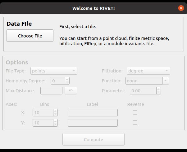
CHAPTER 5

 Getting Started with RIVET

The RIVET software consists of two separate but closely related executables: rivet_console, a command-line pro-
gram, and rivet_GUI, a GUI application. rivet_console is the computational engine of RIVET; it implements the
computation pipeline described in the previous section. rivet_GUI is responsible for RIVET’s visualizations and also
provides a convenient graphical front-end to the functionality of rivet_console. Thanks to this front-end, RIVET’s
visualizations can be carried out entirely from within rivet_GUI.
For new users looking to acquaint themselves with RIVET, we recommend starting by using rivet_GUI to explore
RIVET’s visualization capabilities. In this section, we provide a simple introduction to running RIVET via rivet_GUI.
Later sections of the documentation provide more detail on how to use rivet_console and rivet_GUI. Users who
wish to use RIVET for purposes other than visualization (e.g. machine learning or statistics applications) will want
to familiarize themselves with the command-line syntax of rivet_console, but we recommend all users read this
introduction first.

5.1 Getting started with rivet_GUI

When the user runs rivet_GUI, the following window opens:

 15
RIVET Documentation, Release 1.0

To start a computation, we first select a file by clicking the Choose File button. RIVET can handle several different
types of input: Point clouds, finite metric spaces, simplicial bifiltrations, and short chain complexes. These file formats
for these input types are discussed in detail in Input Data Files.
In this introduction, we consider just one simple type of input file, a CSV file specifying a point cloud in R . Each
line of the file gives the coordinates of one point; these coordinates are written as numbers separated by commas or
white space.
We will use the file data/Test_Point_Clouds/circle_300pts_nofunction.csv from the RIVET repository. This file spec-
ifies 300 points in R2 . The first five lines of the file are as follows:

1.57,2.40
1.21,2.70
0.79,-2.44
-2.44,-2.24
-2.54,-1.25

The 300 points in the file data/Test_Point_Clouds/circle_300pts_nofunction.csv form a noisy circle in R2 , as pictured
below.

16 Chapter 5. Getting Started with RIVET
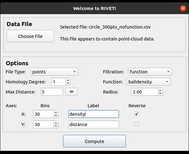
RIVET Documentation, Release 1.0

We will use RIVET to compute a ball density function on this data set, and construct the function-Rips bifiltration
with respect to . (See Function-Rips Bifiltration for the definitions of these terms.) The 1st persistent homology
module of the function-Rips bifiltration of this data algebraically detects the presence of a “loop” in the data. Below,
we illustrate how RIVET visualizes this persistence module.
Upon selecting a file, RIVET activates the input selectors in the Options panel of the dialog box. The following figure
shows RIVET file input window, with the selection of options we will use in this example.

5.1. Getting started with rivet_GUI 17
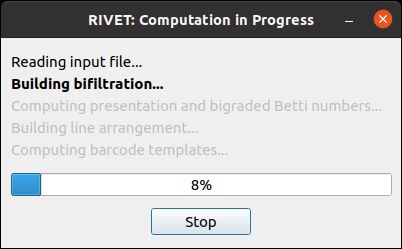
RIVET Documentation, Release 1.0

We now briefly discuss the available options.
The File Type selector tells RIVET what type of input file it should expect. For this data file, we must select the default
option, points.
The Homology Degree selector chooses the degree of the homology module RIVET computes. (Currently, RIVET
computes only a single degree of homology at a time. A user who wishes to examine homology in multiple degrees,
e.g., in degrees 0 and 1, will need to run multiple RIVET computations on the same input data.) Since we want to
discern a “loop” in the data, in this example we select homology degree 1.
The Max Distance selector specifies the maximum length of edges that RIVET will include in the bifiltration it con-
structs. This controls the size of the bifiltration, and thus the cost of the computation. We choose a max distance of 5
for our example. The max distance can be set to infinity, so that every possible edge appears in the bifiltration; this is
done by typing “inf” or clicking on the button with an infinity symbol. The default max distance is infinity.
Three input selectors on the right side of the box determine what bifiltration RIVET will build from the point cloud.
The Filtration selector offers two options: degree and function. The degree option builds a degree-Rips filtration, as
described in Degree-Rips Bifiltration. Here, we choose the function option to build a function-Rips bifiltration.
The function-Rips bifiltration depends on the choice of a real-valued function on the point cloud, which is specified
by the Function selector. Here, we choose the balldensity option, which specifies the function to be a ball density
function. Other options for the function include a Gaussian density function, an eccentricity function, and a user-
defined function, which must be specified in the input file; see Input Data Files for details.
The ball density function depends on a choice of radius parameter, which must be provided in the box below the
Function selector. Here, we choose a radius of 2.
The selectors in the lower portion of the Options box deal with the coordinate axes. The Bins selectors specify the
coarsening of the homology module, as described in Coarsening a Persistence Module. The number of bins is set
separately for the x-axis and the y-axis. The coarsening controls the number of distinct bigrades where generators and
relations of the module can appear. Thus, specifying a smaller number of bin values will speed the RIVET computation
and reduce its memory, but will result in less accurate approximation to the uncoarsened homology module. In this
example, we set both bin values to 30, though higher values could also be used without difficulty.
Next, the user may specify the Label for each axis in the RIVET visualization. For a function-Rips filtration, RIVET
presents the function values along the x-axis. Since we are computing a density estimator, we enter “density” for the
x-axis label. We keep the default “distance” label for the y-axis.
Lastly, the Reverse checkboxes allow the user to reverse axis directions. For example, when using a density function,
we typically want points with larger density values to enter the bifiltration before points with smaller density values;
thus, when we select the “balldensity” function, the Reverse box for the x-axis is checked by default. It is not possible
to reverse the distance axis for a Rips filtration, so in this example, the y-axis Reverse selector is unavailable.
We now click Compute at the bottom of the file input window. This starts the RIVET computational pipeline, as
described in Computation Pipeline. A progress box appears, as shown below.

18 Chapter 5. Getting Started with RIVET
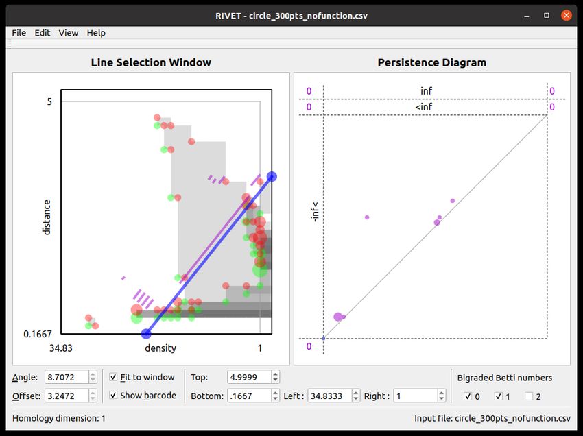
RIVET Documentation, Release 1.0

5.2 Overview of the RIVET Visualization

When the computation finishes, RIVET displays the following visualization. This section gives a brief overview of
the visualization elements; much more detail is found in The RIVET Visualization: Further Details.
The RIVET visualization contains two main windows, the Line Selection Window and the Persistence Diagram Win-
dow, shown in the screenshot below.

5.2.1 Line Selection Window

The Line Selection Window visualizes the Hilbert function values and the bigraded Betti numbers of a bipersistence
module. In addition, it can interactively display the barcode obtained by restricting the module to an affine line. The
viewable region is chosen as described in The RIVET Visualization: Further Details, and can be adjusted using the
controls at the bottom of the window.
The Hilbert function is represented via grayscale shading of the viewable region, and points in the supports of 0 ,
 1 , and 2 are marked with translucent green, red, and yellow dots, respectively. The area of each dot is proportional
to the corresponding function value. Hovering the mouse over a pixel in the window gives a popup box with the value
of the Hilbert function or the bigraded Betti numbers at that point.
A key feature of the RIVET visualization is the ability to interactively select the line via the mouse and have the
barcode ℬ( ) update in real time. The Line Selection Window contains a blue line of non-negative slope, with
endpoints on the boundary of the displayed region of R2 . RIVET displays a barcode for in the line selection
window, provided the “show barcode” box is checked below. The intervals in the barcode for are displayed in
purple, perpendicularly offset from the line . Clicking and draging the blue line with the mouse changes the choice

5.2. Overview of the RIVET Visualization 19
RIVET Documentation, Release 1.0

of line ; for details, see The RIVET Visualization: Further Details. As the line moves, both the barcode in the Line
Selection Window and its persistence diagram representation in the Persistence Diagram Window are updated in real
time.

5.2.2 Persistence Diagram Window

The Persistence Diagram Window displays a persistence diagram representation of the barcode for . The multi-
plicity of a point in the persistence diagram is proportional to the area of the corresponding dot. Additionally, hovering
the mouse over a dot produces a popup that displays the multiplicity of the dot.
The bounds for the square viewable region (surrounded by dashed lines) in this window are chosen automatically.
They depend on the bounds of the viewable region in the slice diagram window, but not on . Some points in the
persistence diagram may have coordinates that fall outside of the viewable region. These points are indicated by dots
or numbers along the left and top edges of the persistence diagram. For details, see The RIVET Visualization: Further
Details.

5.2.3 Customizing the Visualization

The look of the visualization can be customized by choosing RIVET → Preferences on Mac, or Edit → Configure on
Linux, and adjusting the settings there.

20 Chapter 5. Getting Started with RIVET
CHAPTER 6

 Running RIVET from the Console

As mentioned on the Getting Started with RIVET page, RIVET can be run from the console via the executable
rivet_console. This executable has three main functions:
 • Given an input data file in one of the formats described in the Input Data Files section of this documentation,
 rivet_console can compute a file called the module invariants (MI) file. The MI file stores the Hilbert function,
 bigraded Betti numbers, and augmented arrangement of a persistent homology module of the input data. The
 MI file is used by the RIVET visualization, and also for the following:
 • Given an MI file of a bipersistence module and a second file, the line file, specifying a list of lines,
 rivet_console prints the barcodes of the 1-D slices of each line to the console. The computations are performed
 using fast queries of the augmented arrangement of .
 • Given an input data file as input, rivet_console can print a minimal presentation of a persistent homology
 module of the input data. It can also print the Hilbert function and Bigraded Betti numbers.
In version 1.1 of RIVET, the syntax for running rivet_console and the format requirements for input files have been
redesigned to be more flexible and user-friendly. rivet_GUI’s interface for computing MI files has also been updated
accordingly. However, rivet_console is backwards-compatible with older input files.
In what follows, we explain in more detail how to use rivet_console. The syntax for running rivet_console is also
described in the executable’s help information, which can be accessed via the command:
rivet_console (-h | --help)

The help information also describes some additional technical functionality of rivet_console that we will not discuss
here.

6.1 Computing a Module Invariants File

Here the basic syntax for computing a module invariants file:
rivet_console [options]

 • is an input data file;

 21
RIVET Documentation, Release 1.0

 • is the name of the module invariants file to be computed.
 • [options] are command-line flags control the computation, as specified below.
For example, a typical call to rivet_console to compute an MI file MI_output.rivet from an input file my_data.txt might
look as follows:

rivet_console input.txt output.rivet --datatype metric --homology 1 --xbins 100 --
 ˓→ybins 100

 • --datatype metric tells RIVET that input.txt contains a distance matrix (specifying a finite metric space).
 • --homology 1 tells RIVET to consider persistent homology in degree 1.
 • --xbins 100 and --ybins 100 tell RIVET to compute a coarsened version of the homology module such
 that the support of the 0th and 1st Betti numbers lies on a 100x100 grid in R2 . (This is done for the sake of
 computational efficiency.)
When called in this way, rivet_console constructs the degree-Rips bifiltration of the metric space.

6.2 Command-Line Flags for Use with Input Data Files

We now explain in detail rivet_console’s use of command-line flags to control computations taking an input data file
as input.
Command-line flags can be placed in the input data file itself, rather than given on the command line. Flags in the
input data file must be provided in the top lines of the file, before the data is given. It is possible to specify flags both
in the file and on the command line. If the same flag is given in both the input data file and the command line, then
rivet_console ignores the copy of the flag in the input file and uses the flag given on the command line. Whether on
the command line or in an input file, flags can appear in any order.
The most important flags are the following:
 • --datatype specifies the type of data contained in the input file. The default is points. For
 details, see Input Data Files.
 • -H or --homology specifies degree of homology to compute. If un-
 specified, the default value is zero. (RIVET handles only one homology degree at a time.)
 • -x and -y specify the dimensions of the grid used for coarsening. The grid spacing
 is taken to be uniform in each dimension. (For details on grids and coarsening, see Coarsening a Persistence
 Module.) If unspecified, each flag takes a default value of 0, which means that no coarsening is done at all in that
 coordinate direction. However, to control the size of the augmented arrangement, most computations of a MI
 file should use some coarsening of the module. These flags can also be specified in the longer forms --xbins
 . and --ybins .
 • --bifil specifies the type of bifiltration to be built. Specifying a bifiltration type only makes sense
 for certain input data types, and hence this flag can only be used for such input. In cases where the flag can be
 used, the available bifiltration types are function and degree. The default depends on the choice of input
 data type. For details, see the Input Data Files section of this documentation.
 • --function tells RIVET to construct a function-Rips bifiltration using the function . RIVET
 supports both user-specified functions and three built-in function types. The options for are as follows (see
 Function-Rips Bifiltration for definitions). The built-in functions each depend on a parameter, which is specified
 in square brackets. The square brackets are required, even if the user chooses not to specify the parameter value,
 in which case RIVET uses a default parameter value. (The user is encouraged to view the empty square brackets
 as a reminder that they are choosing the default parameter value.) The supported functions are:

22 Chapter 6. Running RIVET from the Console
RIVET Documentation, Release 1.0

 – balldensity[r], where r is a positive decimal number, for a closed-ball density function with radius
 parameter r. If balldensity[] is entered, the default value of r is taken to be the 20th percentile of
 all non-zero distances between points. The filtration direction for this function is automatically set to be
 descending.
 – gaussian[ ], where is a positive decimal number, for a gaussian density functor with standard devi-
 ation . If gaussian[] is entered, the default value of is chosen in the same way that the default radius
 value for the ball density estimator is chosen. The filtration direction is set to be descending.
 – eccentricity[p], where p is the exponent for the eccentricity function. If eccentricity[] is
 entered, p is set to the default value of 1. The filtration direction is set to be descending.
 – user. This option requires that the input data file specify a function, as explained in Input Data Files. If a
 function is provided in the file, the user-specified function is used by default, so it is in fact never necessary
 to use this flag, but it can be included for clarity’s sake. Specifying a user-defined function directly from
 the command line is not supported.
The following flags are also available, and are useful in many cases:
 • --maxdist specifies the maximum distance to be considered when building a Vietoris-Rips
 bifiltration. Any edge whose length is greater than this distance will not be included in the complex. If unspeci-
 fied, this flag takes the default value of infinity. Choosing a small value for reduces the amount
 of memory required for the computation, relative to the default.
 • When computing an MI file, --xlabel and --ylabel respectively specify labels
 for the -axis and -axis in the rivet_GUI visualization window. The labels are stored as metadata in the MI
 file. If either of these flags are not given, RIVET provides default labels, which depend on the input data type
 and (where applicable), the type of bifiltration being constructed. For example, when constructing a degree-Rips
 filtration, the default labels for the -axis and -axis are degree and distance, respectively.
 • --xreverse and --yreverse reverse the direction of the -axis and -axis, respectively. Reversing an
 axis direction only makes sense for certain bifiltration constructions, and hence these flags can only be used
 in certain circumstances. For example, for a function-Rips filtration, the -axis indexes the function threshold
 parameter in RIVET’s visualization, while the y-axis indexes the scale parameter. In general, it makes equal
 sense to construct a function-Rips bilftration with respect to increasing or decreasing function values; the flag
 --xreverse tells RIVET to use decreasing values. But we don’t have a good way of building a function-
 Rips bifiltration using a decreasing scale parameter, so --yreverse is not available for the construction of a
 function-Rips bifiltration; including this flag has no effect. See Input Data Files for the specifics of when and
 how --xreverse and --yreverse can be used.
Some additional flags which concern the internals of RIVET’s computations are also available, but can be disregarded
by most users:
 • --num_threads This flag specifies the maximum number of threads to use for parallel
 computation. The default value is 0, which lets OpenMP decide how many threads to use.
 • -V or --verbosity This flag controls the amount of text that
 rivet_console prints to the terminal window. The verbosity may be specified as an integer between 0 and 10:
 greater values produce more output. A value of 0 results in minimal output, a value of 10 produces extensive
 output.
 • -k or --koszul This flag causes RIVET to use a koszul homology-based algorithm to compute the Betti
 numbers, instead of the default approach based on computing a minimal presentation.

6.3 Computing Barcodes of 1-D Slices

Here is the basic syntax for computing the barcodes of 1-D slices of a bipersistence module, given an MI file as input:

6.3. Computing Barcodes of 1-D Slices 23
RIVET Documentation, Release 1.0

rivet_console --barcodes

 is a file specifying a list of affine lines in R2 with non-negative slope. Each line is specified by its
angle and offset parameters. The following diagram shows these parameters for a particular line, with angle denoted
 and offset denoted .

As the diagram indicates, is the angle between the line and the horizontal axis in degrees (0 to 90). The offset
parameter is the signed distance from the line to the origin, which is positive if the line passes above/left of the origin
and negative otherwise. This choice of parameters makes it possible to specify any line of nonnegative slope, including
vertical lines.
The following gives a sample line file:

#A line that starts with a # character will be ignored, as will blank lines
23 -0.22
67 1.88
10 0.92
#100 0.92 90

For each line specified in , rivet_console will print barcode information as a single line of text,
beginning by repeating the query parameters. For example, output corresponding to the sample line file above might
be:

23 -0.22: 88.1838 inf x1, 88.1838 91.2549 x5, 88.1838 89.7194 x12
67 0.88: 23.3613 inf x1
10 0.92: 11.9947 inf x1, 11.9947 19.9461 x2, 11.9947 16.4909 x1, 11.9947 13.0357 x4

The barcodes are given with respect to an isometric parameterization of the query line that takes zero to be the inter-
section of the query line with the nonnegative portions of the coordinate axes; there is a unique such intersection point
except if the query line is one of the coordinate axes, in which case we take zero to be origin.
Furthermore, barcodes are returned as multisets of intervals. For example, in the sample output above, 88.1838
inf x1 indicates a single interval [88.1838, ∞).

6.4 Printing a Minimal Presentation

The basic syntax for computing and printing minimal presentation of a bipersistence module is the following:

rivet_console --minpres [command-line flags]

24 Chapter 6. Running RIVET from the Console
RIVET Documentation, Release 1.0

 • is an input data file;
 • [command-line flags] work as specified above, in Command-Line Flags for Use with Input Data Files.
The following example shows the output format for the minimal presentation:

x-grades
3
7/2
4

y-grades
0
1
2

MINIMAL PRESENTATION:
Number of rows:2
Row bigrades:
| (1,0) (0,1) |
Number of columns:3
Column bigrades:
| (1,1) (2,1) (1,2) |
0 1
1
0

The first few lines give lists of possible x- and y-grades of generators and relations in the presentation. (NOTE: With
the current code, these lists may not be minimal; we plan to change this soon.)
The next lines specify the bigrades of the generators and relations, via indices for the lists of x- and y-grades. Lists are
indexed from 0. Thus, in this example, the row bigrades specified are (7/2,0) and (3,1).
The final three lines specify columns of the matrix in sparse format. Rows are indexed from 0. Hence, the matrix
specified is:

1 0 1
1 1 0

NOTE: It would be better design to have the minimal presentation printed in the format of the FIrep datatype de-
scribed on the Input Data Files page. But as this would require some restructuring of the code, this has not yet been
implemented.

6.5 Printing Hilbert Function and Bigraded Betti Numbers

Here is the basic syntax for computing both the Hilbert function and bigraded Betti numbers of a bipersistence module:

rivet_console --betti [command-line flags]

As above,
 • is an input data file;
 • [command-line flags] work as specified above, in Command-Line Flags for Use with Input Data Files.
NOTE: Currently, one cannot print the Hilbert function and bigraded Betti numbers of a module separately. Nor can
one print the minimal presentation, Betti numbers, and Hilbert Function together. This will change in the future.

6.5. Printing Hilbert Function and Bigraded Betti Numbers 25
RIVET Documentation, Release 1.0

The following shows the output format for the Hilbert function and bigraded Betti numbers, for the minimal presenta-
tion in the example above:

x-grades
3
7/2
4

y-grades
0
1
2

Dimensions > 0:

(0, 1, 1)
(0, 2, 1)

(1, 0, 1)
(1, 1, 1)
(1, 1, 1)

(2, 0, 1)

Betti numbers:
xi_0:
(1, 0, 1)
(0, 1, 1)
xi_1:
(1, 1, 1)
(1, 2, 1)
(2, 1, 1)
xi_2:
(2, 2, 1)

The first few lines give lists of possible x- and y-grades of non-zero Betti numbers. This defines a finite grid ∈ R2 .
The next few lines specify the points in where the Hilbert function is non-zero, together with the value of the Hilbert
function at each point. For each such point, a triple (x-index, y-index, value) is printed. (Note that this information in
fact determines the Hilbert function at all points in R2 .)
The remaining lines specify the points where the Betti numbers are non-zero, along with the value of the Betti number
at that point. (0th, 1st, and 2nd Betti numbers are handled separately.) Again, for each such point, a triple (x-index,
y-index, value) is printed.

26 Chapter 6. Running RIVET from the Console
CHAPTER 7

 The RIVET Visualization: Further Details

In the section Overview of the RIVET Visualization, we gave brief overview of RIVET’s visualization of bipersistence
modules. Here we provide a more detailed description. To make this self-contained, we also revisit the material on
visualization covered earlier.

7.1 Handling MI Files with rivet_GUI

As explained earlier, RIVET’s visualizations are handled by the executable rivet_GUI, and require an MI file as
input. The MI file can be computed by a direct call to rivet_console, as explained on the Running RIVET from the
Console page, and then opened in rivet_GUI. Alternatively, rivet_GUI can call rivet_console to compute the MI file.
(The example on the Getting Started with RIVET page is an instance of the latter approach, though MI files were not
explicitly mentioned there.)
When the user runs rivet_GUI, a window opens which allows the user to select a file. This file can be either an input
data file in one of the input formats described in Input Data Files, or an MI file.
If an input data file is chosen, the GUI allows the user to graphically select options for computation of a MI file, as we
have seen earlier on the Getting Started with RIVET page. Most options that can be selected via a command line flag,
as described on the Running RIVET from the Console page, can also be selected in the GUI. (However, some technical
options, such as choosing the maximum number of cores to use in a parallel computation, are not available through
the rivet_GUI.) After the user clicks the Compute button, the MI file is computed via a call to rivet_console and
the visualization is started. (Note that after the Hilbert Function and Betti numbers are shown in the visualization, it
may take a significant amount of additional time to prepare the interactive visualization of the barcodes of 1-D slices.)
Using the File menu in the GUI, the user may save the MI file; a module invariants file computed by rivet_GUI is not
saved automatically.
If an MI file is selected in the file dialogue window, the data in the file is loaded immediately into the RIVET visual-
ization, and the visualization begins.

 27
RIVET Documentation, Release 1.0

7.2 Line Selection Window

The RIVET interface contains two main windows, the Line Selection Window and the Persistence Diagram Window,
shown in the screenshot below.

The Line Selection Window not only visualizes the Hilbert function values and the bigraded Betti numbers of a biper-
sistence module , but also allows the user to choose linear slices along which barcodes are displayed.
By default, the Line Selection Window plots a rectangle in R2 containing the union of the supports of bigraded Betti
number functions , ∈ {0, 1, 2}. (If the input to RIVET is an FIRep and the Betti numbers are not supported on
a horizontal or vertical line, this will be the smallest such rectangle. If the input is a point cloud, metric space, or
bifiltration, and the birth indices of all simplices in the bifiltration do not lie on a single line, the rectangle will be the
smallest one containing the birth indices of all simplices.)
The Hilbert function values are plotted using grayscale shading. Specifically, the greyscale shading at a point in this
rectangle represents dim : is unshaded when dim = 0, and larger dim corresponds to darker shading.
Hovering the mouse over brings up a popup box which gives the precise value of dim .
Points in the supports of 0 , 1 , and 2 are marked with green, red, and yellow dots, respectively (though these
colors are customizable via the Edit menu on Linux or the Preferences menu on Mac). The area of each dot is
proportional to the corresponding function value. The dots are translucent, so that, for example, overlaid red and green
dots appear brown on their intersection. This allows the user to read the values of the Betti numbers at points which
are in the support of more than one of the functions. Furthermore, hovering the mouse over a dot produces a popup
box that gives the values of the bigraded Betti numbers at that point.
A key feature of the RIVET visualization is the ability to interactively select the line via the mouse and have the
barcode ℬ( ) update in real time. The Line Selection Window contains a blue line of non-negative slope, with

28 Chapter 7. The RIVET Visualization: Further Details
RIVET Documentation, Release 1.0 endpoints on the boundary of the displayed region of R2 . RIVET displays a barcode for in the line selection window, provided the “show barcode” box is checked below. The intervals in the barcode for are displayed in purple, perpendicularly offset from the line . The user can click and drag the blue line with the mouse to change the choice of line . Clicking and dragging an endpoint of the line moves that endpoint while keeping the other fixed. One endpoint is locked to the top and right sides of the displayed rectangle; the other endpoint is locked to the bottom and left sides. Clicking and dragging the interior of the line (away from its endpoints) moves the line as follows: • Left-clicking moves the line in the direction perpendicular to its slope, keeping the slope constant. • Right-clicking changes the slope of the line, while keeping the bottom/left endpoint fixed. As the line moves, both the barcode in the Line Selection Window and its persistence diagram representation in the Persistence Diagram Window are updated in real time. The Angle and Offset controls below the Line Selection Window can also be used to select the line. The coordinate bounds of the viewable rectangle may be adjusted using the Top, Bottom, Left, and Right control boxes at the bottom of the RIVET window. The window can be reset to the default by choosing View → Restore Default Window. Choosing View → Betti number window sets the window to the smallest rectangle containing all non-zero Betti numbers. 7.3 Persistence Diagram Window The Persistence Diagram Window (at right in the screenshot above) displays a persistence diagram representation of the barcode for . The bounds for the square viewable region (surrounded by dashed lines) in this window are chosen automatically. They depend on the bounds of the viewable region in the slice diagram window, but not on . Let the square [0, ] × [0, ] be the viewable region. It may be that the barcode contains some intervals [ , ) with either or not contained in [0, ]. To represent such intervals on the screen, RIVET displays some information at the top and left of the persistence diagram which is not found in typical persistence diagrams. Above the square region of persistence diagram are two narrow horizontal strips, separated by a dashed horizontal line. The upper strip is labeled inf, and the lower strip is labeled inf. RIVET plots a point in the upper strip for each interval [ , ∞) in the barcode with 0 ≤ ≤ . RIVET plots a point in the lower strip for each interval [ , ) in the barcode with 0 ≤ ≤ ∞). To the left of the square region of persistence diagram is a vertical strip labeled - inf . RIVET plots a point in this strip for each interval [ , ) in the barcode with 0 ≤ ≤ ). Just to the right and to the left of each of the two upper horizontal strips is a number, separated from the strip by a dashed vertical line: • To the upper right is the number of intervals [ , ∞) in the barcode with . • To the lower right is the the number of intervals [ , ) with and ∞. • To upper left is the number of intervals [ , ∞) with 0. • To the lower left is the number of intervals [ , ) with < 0 and ∞. Finally, there is a number in the bottom left corner of the persistence diagram window. This is the number of intervals [ , ) with < 0. As with the bigraded Betti numbers in the Line Selection Window, the multiplicity of a point in the persistence diagram is indicated by the area of the corresponding dot. Additionally, hovering the mouse over a dot produces a popup that displays the multiplicity of the dot. 7.3. Persistence Diagram Window 29
You can also read