Adversarial Domain Randomization
←
→
Page content transcription
If your browser does not render page correctly, please read the page content below
Adversarial Domain Randomization

                                                                             Rawal Khirodkar            Kris M. Kitani
                                                                                    Carnegie Mellon University
                                                                                     {rkhirodk,kkitani}@cs.cmu.edu
arXiv:1812.00491v2 [cs.CV] 29 Aug 2021

                                                                  Abstract

                                             Domain Randomization (DR) is known to require a signif-
                                         icant amount of training data for good performance [20, 49].
                                         We argue that this is due to DR’s strategy of random data
                                         generation using a uniform distribution over simulation pa-
                                         rameters, as a result, DR often generates samples which are
                                         uninformative for the learner. In this work, we theoretically
                                         analyze DR using ideas from multi-source domain adapta-
                                         tion. Based on our findings, we propose Adversarial Domain
                                         Randomization (ADR) as an efficient variant of DR which
                                         generates adversarial samples with respect to the learner                           (a) Domain Randomization (DR)
                                         during training. We implement ADR as a policy whose action
                                         space is the quantized simulation parameter space. At each
                                         iteration, the policy’s action generates labeled data and the
                                         reward is set as negative of learner’s loss on this data. As a
                                         result, we observe ADR frequently generates novel samples
                                         for the learner like truncated and occluded objects for object
                                         detection and confusing classes for image classification. We
                                         perform evaluations on datasets like CLEVR, Syn2Real, and
                                         VIRAT for various tasks where we demonstrate that ADR
                                         outperforms DR by generating fewer data samples.

                                         1. Introduction
                                             A large amount of labeled data is required to train deep                (b) Adversarial Domain Randomization (ADR)
                                         neural networks. However, a manual annotation process
                                         on such a scale can be expensive and time-consuming, es-             Figure 1. We compare synthetic images generated by DR and ADR
                                                                                                              along with their instance segmentation maps for the task of object
                                         pecially for complex vision tasks like semantic segmenta-
                                                                                                              detection. ADR learns to generate harder samples containing oc-
                                         tion where labels are difficult to specify. It is, thus, natu-       cluded and truncated objects. This allows efficient learning with
                                         ral to explore simulation for generating synthetic data as a         few samples.
                                         cheaper and quicker alternative to manual annotation. How-
                                         ever, while use of simulation makes data annotation easier,          domain to bridge the gap. DA assumes access to unlabeled
                                         it results in the problem of domain gap. This problem arises         target data and achieves domain invariant feature extraction
                                         when the training data distribution - source domain differs          by explicitly minimizing feature discrepancy between source
                                         from the test data distribution - target domain. In this case,       and target data. On the other hand, in the absence of unla-
                                         learners trained on synthetic data would suffer from high            beled target data, DR bridges the gap by adding enough
                                         generalization error. There are two popular solutions to             variations (e.g. random textures onto objects for detection)
                                         reducing domain gap, (1) the well studied paradigm of do-            to source domain. These variations force the learner to focus
                                         main adaptation (DA) [53] and (2) the recently proposed              on essential domain invariant features.
                                         domain randomization (DR) [48]. Both the solutions focus                 A natural question therefore arises: how does DR com-
                                         on extracting domain invariant features from labeled source          pensate for the lack of information on target domain? The

                                                                                                          1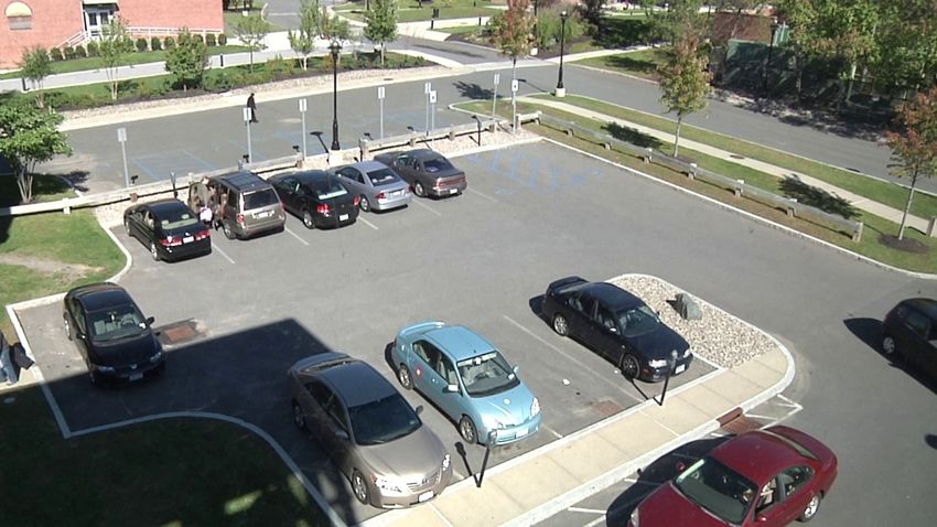
answer lies in the design of the simulator used by DR for         policy to generate data which is consistent with target data.
randomization. The simulator is encoded with target do-           As a result, we no longer need to manually encode domain
main knowledge (e.g. priors on shape of objects) beforehand.      knowledge in the design of the simulator. In summary, the
This acts as a sanity check between the labels of source do-      contributions of our work are as follows:
main and target domain (e.g. cars should not be labeled as
trucks). Another key design decision involves which simula-       • Theoretical Analysis for Domain Randomization: We
tion parameters are supposed to be randomized. This plays           present a theoretical perspective on effectiveness of DR.
an important role in deciding the domain invariant features         We also provide a bound for its generalization error and
which help the learner in generalizing to the target domain.        analyze its limitations.
Clearly, these domain invariant features are task dependent,      • Adversarial Domain Randomization: As a solution to
as they contain critical information to solve the task. e.g.        DR’s limitations, we propose a more data efficient variant
in car detection, the shape of a car is a critical feature and      of DR, namely ADR.
has to be preserved in source domain, it is therefore accept-     • Evaluations on Real Datasets for Diverse Tasks: We
able to randomize the car’s appearance by adding textures           benchmark our approach on image classification and ob-
in DR. However, when the task changes from car detection            ject detection on real-world datasets like Syn2Real [30],
to a red car detection, car’s appearance becomes a critical         VIRAT [29].
feature and can no longer be randomized in DR. We believe
it is important to understand such characteristics of the DR      2. Related Work
algorithm. Therefore, as a step in this direction, in section
3, we provide theoretical analysis of DR. Concretely our             Our work is broadly related to approaches using a sim-
analysis answers the following questions about DR: 1) how         ulator as a source of supervised data and solutions for the
does it make the learner focus on domain invariant features?      reduction of domain gap.
2) what is its generalization error bound? 3) in presence of      Synthetic Data for Training Recently with the advent of
unlabeled target data, can we use it with DA? 4) what are its     rich 3D model repositories like ShapeNet and the related
limitations?                                                      ModelNet [6], Google 3D warehouse [1], ObjectNet3D [55],
    In our analysis, we identify a key limitation: DR requires    IKEA3D [24], PASCAL3D+ [56] and increase in accessi-
a lot of data to be effective. This limitation mainly arises      bility of rendering engines like Blender3D, Unreal Engine
from DR’s simple strategy of using a uniform distribution for     4 and Unity3D, we have seen a rapid increase in using syn-
simulation parameter randomization. As a result, DR often         thetic data for performing visual tasks like object classifi-
generates samples which the learner has already seen and          cation [30], object detection [30, 49, 15], pose estimation
is good at. This wastes valuable computational resources          [42, 22, 44], semantic segmentation [52, 39] and visual ques-
during data generation. We can view this as an exploration        tion answering [19]. Often the source of such synthetic data
problem in the space of simulation parameters. A uniform          is a simulator, and use of simulators for training control
sampling strategy in this space clearly does not guarantee suf-   policies is already a popular approach in robotics [5, 47].
ficient exploration in image space. We address this limitation    SYNTHIA [37], GTA5 [36], VIPER [35], CLEVR [19], Air-
in section 4 by proposing Adversarial Domain Randomiza-           Sim [41], CARLA [11] are some of the popular simulators
tion (ADR), a data efficient variant of DR. ADR generates         in computer vision.
adversarial samples with respect to the learner during train-     Domain Adaptation: Given source domain and target do-
ing. We implement ADR as a policy whose action space is           main, methods like [4, 8, 16, 17, 57, 28, 50] aim to reduce
the quantized simulation parameter space. At each iteration,      the gap between the feature distributions of the two domains.
the policy is updated using policy gradients to maximize          [4, 14, 13, 50, 17] did this in an adversarial fashion using
learner’s loss on generated data whereas the learner is up-       a discriminator for domain classification whereas [51, 27]
dated to minimize this loss. As a result, we observe ADR          minimized a defined distance metric between the domains.
frequently generates samples like truncated and occluded          Another approach is to match statistics on the batch, class or
objects for object detection and confusing classes for im-        instance level [17, 7] for both the domains. Although these
age classification. Figure 1 shows a comparison of sample         approaches outperform simply training on source domain,
images generated by DR and ADR for the task of object             they all rely on having access to target data albeit unlabelled.
detection.                                                        Domain Randomization: These methods [38, 10, 48, 18,
   Finally, we go back to the question posed previously, can      49, 32, 31, 46, 44, 20] do not use any information about
we use DR with DA when unlabeled target data is available?        the target domain during training and only rely on a simula-
Our reinforcement learning framework for ADR easily ex-           tor capable of generating varied data. The goal is to close
tends to incorporate DA’s feature discrepancy minimization        the domain gap by generating synthetic data with sufficient
in form of reward for the policy. We thus incentivize the         variation that the network views real data as just another
variation. The underlying assumption here is that simula-          source domain. The error of a hypothesis PN  h on this source
tor encodes the domain knowledge about the target domain           domain (α-error) is denoted as α (h) = i=1 αi i (h). The
                                                                                                             PN
which is often specified manually [33].                            α input distribution is denoted as Dα = i=1 αi Di .
                                                                      The multiple source domain problem can now be reduced
3. Theoretical Analysis of DR                                      to training on labeled samples from α-source domain for
                                                                   various values of α ∈ ∆. We use Dα to sample inputs
   We analyze DR using generalization error bounds from
                                                                   from X , which are then labeled using all the labeling func-
multiple source domain adaptation [2]. The key insight is to
                                                                   tions {hfi i}|N
                                                                                 i=1 . We learn a hypothesis h to minimize the
view DR as a learning problem from multiple source domains                                      PN
                                                                   empirical α-error, ˆα (h) = i=1 αi ˆi (h).
where each source domain represents a particular subset of
the data space. For example, consider the space of all car         Generalization Error Bound. Let ĥα = argminh ˆα (h)
images. The images containing a car of a particular make           and h∗α = argminh α (h) i.e. ĥα and h∗α minimize the em-
form a subset of that space which we refer to as a single          pirical and true α-error respectively. We are interested in
source domain. If one were to generate random images               bounding the generalization error T (ĥα ) for empirically op-
across different car makes, as we do in DR, this can be            timal hypothesis ĥα . However, using Hoeffding’s inequality
interpreted as combining data from multiple source domains.        [40], it can be shown that minimum empirical error ˆα (ĥα )
   In this section, we first introduce the preliminaries in        converges uniformly to the minimum true error α (h∗α ) i.e.
3.1 followed by a formal definition of DR algorithm in 3.2.        without loss of generality ĥα converges to h∗α given large
Lastly, we draw parallels between DR and multiple source           number of samples. To simplify our analysis we instead
domain adaptation in 3.3 where we also show that the gen-          bound generalization error T (h∗α ) for true optimal hypoth-
eralization error bound for DR is better than the bound for        esis h∗α (the bound for ĥα is provided in supplementary
data generation without randomization.                             material).
                                                                      Following the proof for Th. 5 (A bound using combined
3.1. Preliminaries
                                                                   divergence) in [2], we provide a bound for generalization
    The notation introduced below is based on the theoretical      error T (h∗α ) below.
model for DA using multiple sources for binary classification
[2]. The analysis here is limited to binary classification for     Theorem 1. (Based on Th.5 [2]) Consider the optimal
simplicity but can be extended to other tasks as long as the       hypothesis on target domain h∗T = argminh T (h) and
triangle inequality holds [3].                                     on α-source domain h∗α = argminh α (h). If γα =
    A domain is defined as a tuple hD, f i where: (1) D is         minh {T (h) + α (h)}, then
a distribution over input space X and (2) f : X 7→ Y is a
                                                                          T (h∗α ) ≤ T (h∗T ) + 2γα + dH∆H (Dα , DT )
labeling function, Y being the output space which is [0, 1]
for binary classification. N source domains are denoted as         Remarks: Proof in supplementary material. T (h∗T ) is the
{hDi , fi i}|N
             i=1 and the target domain is denoted as hDT , fT i.   minimum true error possible for the target domain (clearly,
A hypothesis is a binary classification function h : X 7→          T (h∗T ) ≤ T (h∗α )). γα represents the minimum error using
{0, 1}. The error (sometimes called risk) of a hypothesis h        both the target domain and α-source domain jointly. Intu-
                       f under distribution
w.r.t a labeling function                      D is defined as    itively, it represents the agreement between all the labeling
(h, f, D) := Ex∼D |h(x) − f (x)| . We denote the error of         functions involved (target domain and all source domains) i.e.
hypothesis h on target domain as T (h) = (h, fT , DT ) and       γα would be large, if these labeling functions label an input
on ith source domain as i (h) = (h, fi , Di ). As common         differently. Lastly, dH∆H (Dα , DT ) is the H∆H divergence
notation in computational learning theory, we use T (h) and       between input distributions Dα and DT . In summary, gener-
ˆT (h) to denote the true error and empirical error on the        alization on target domain T (h∗α ) depends on: (1) difficulty
target domain. Similarly, i (h) and ˆi (h) are defined for ith   of task on target domain T (h∗T ); (2) labeling consistency
source domain.                                                     between target domain and source domains γα ; (3) similar-
Multiple Source Domain Problem. Our goal is to learn               ity of input distribution between target and source domains
a hypothesis h from hypothesis class H which minimizes             dH∆H (Dα , DT ).
T (h) on the target domain hDT , fT i by only using labeled
samples from N source domains {hDi , fi i}|N i=1 .
                                                                   3.2. Domain Randomization
α-Source Domain. We combine N source domains into a                   DR addresses the multiple source domain problem by
single source domain denoted as α-source domain where              modeling various source domains using a simulator with
α helps us control the contribution of each source domain          randomization. The simulator is a generative module which
                 We denote by ∆ the simplex of RN , ∆ =
during training. P                                                 produces labeled data (x, y). In practice, DR uses an accu-
                   N
{α : αi ≥ 0 ∧ i=1 αi = 1}. Any α ∈ ∆ forms an α-                   rate simulator which internally encodes the knowledge about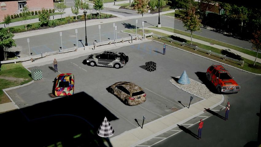
the target domain as a target labeling function fT (x), such                                       S1
                                                                                                                         T
that y = fT (x). Concretely, let Θ be the rendering parame-                                                    d
ter space and DΘ be a probability distribution over Θ. We
                                                                                  S5                    Sα         S2
denote the simulator as a function g : Θ 7→ X × Y such that
g(θ) = {x, y} where θ ∼ DΘ . Simply put, a simulator g
takes a set of parameters θ and generates an image x and its
label y. In general, the DR algorithm generates data by ran-
domly (uniformly) sampling θ from Θ i.e. DΘ is set to UΘ ,                               S4                   S3
an uniform distribution over Θ (refer Alg. 1). The algorithm
outputs a hypothesis ĥ which empirically minimizes the loss        Figure 2. A visualization of the domains using simplex ∆(N = 5).
`(ĥ(xi ), yi ) over M data samples. Note, in our analysis, we      The corners of ∆ are the source domains S1 , . . . , S5 and the point
set `(ĥ(x), y) to be |ĥ(x) − y|. LEARNER - UPDATE is the          T is the target domain. Any interior point Sα ∈ ∆ is the upper
                                                                    bound for generalization error T (h∗α ) and the point T is T (h∗T ).
parameter update of ĥ using loss `(ĥ(xi ), yi ).
                                                                    The distance between Sα and T is d = 2γα + dH∆H (Dα , DT ).
                                                                    The data generated using DR is the centre of ∆.
Algorithm 1 Domain Randomization
    Input: g, M
    Output: ĥ                                                      Lemma 2. For i ∈ {1, . . . , N }, let αi = [0, .. 1 ..0],
                                                                                                                                   ith
 1: for i ∈ {1, 2, . . . , M } do
                                                                    γi = minh {T (h) + i (h)} and ᾱ = [ N1 , N1 ..., N1 ], γ̄ =
 2:     θ ∼ UΘ                                                                       PN
 3:     {x, y} = g(θ)                                               minh {T (h) + N1 i=1 i (h)}, then
 4:     ĥ = LEARNER - UPDATE(ĥ, x, y)                                 N
                                                                     1 X
                                                                           2γi + dH∆H (Di , DT ) ≥ 2γ̄ + dH∆H (Dᾱ , DT )
                                                                     N i=1
The objective function optimized by these steps can be writ-
ten as follows:                                                     Remarks: Proof provided in supplementary material
                       h                 i
             min E ` h g(θ)x , g(θ)y                    (1)         follows from the convexity of distance measure 2γi +
              h∈H θ∼UΘ
                                                                    dH∆H (Di , DT ) with application of Jensen’s inequality [23].
3.3. DR as ᾱ-Source Domain                                         Using this lemma, the corollary 2.1 states that in the absence
                                                                    of unlabeled target data, in expectation DR (centre of ∆) is
    We interpret data generated using DR as labeled data
                                                                    superior to data generation without randomization (any other
from an α-source domain, specifically α = [ N1 , . . . , N1 ]
                                                                    point in ∆).
(referred as ᾱ hereafter). This captures equal contribution
by each sample during training according to Alg 1. Using            Corollary 2.1. The generalization error bound for ᾱ-source
Th. 1, we can bound the generalization error for ᾱ-source          domain (DR) is smaller than the expected generalization
domain (DR) by T (h∗T ) + 2γ̄ + dH∆H (Dᾱ , DT ) where             error bound of a single source domain (expectation over a
                          PN
γ̄ = minh {T (h) + N1 i=1 i (h)}.                                 uniform choice of source domain).
    We now compare DR with data generation without ran-
domization or variations. The later is same as choosing             4. Adversarial Domain Randomization
only one source domain for training, denoted as αi -source
domain where αi is a one-hot N -vector indicating domain               We modify DR’s objective (eq.1) by making a pessimistic
i ∈ {1, . . . , N }. The generalization error bound for αi -        (adversarial) assumption about DΘ instead of assuming it
source domain would be T (h∗T ) + 2γi + dH∆H (Di , DT )            to be stationary and uniform. By making this adversarial
where γi = minh {T (h) + i (h)}.                                  assumption, we force the learned hypothesis to be robust to
    Refer to Fig. 2 for a visualization of generalization er-       adversarial variations occurring in the target domain. This
ror of Sα as a distance measure from target domain, we              type of worst case modeling is especially desirable when
define d = 2γα + dH∆H (Dα , DT ) as the upper bound for             annotated target data is not available for rare scenarios.
|T (h∗α ) − T (h∗T )|. We wish to find an optimal α which            The resulting min-max objective function is as follows:
minimizes this distance measure i.e. the point in ∆ closest                                    h                   i
to the target domain (α2 in Fig. 2). However, when no unla-                    min max E ` h g(θ)x , g(θ)y                     (2)
                                                                                h∈H DΘ θ∼DΘ
beled target data is available it is best to choose the centre of
∆ (α = ᾱ) as our source domain. We prove this in lemma
                                                                    4.1. ADR via Policy Gradient Optimization
2, which states that the distance of target domain from the
centre of ∆ is less than the average distance from the corners         This adversarial objective function is a zero-sum two
of ∆.                                                               player game between SIMULATOR (g) and LEARNER (h).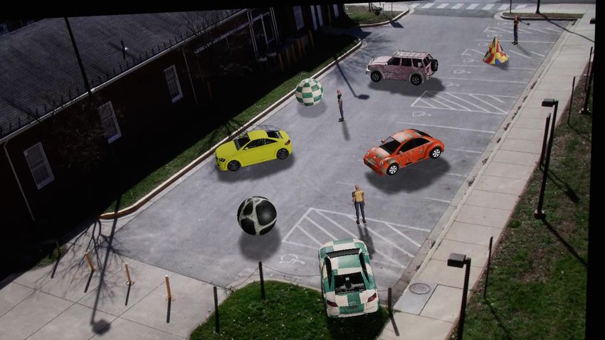
4.2. DA as ADR with Unlabeled Target Data
                                                                         In the original formulation of the ADR problem above,
                                                                      our task was to generate a multi-source data that would
                                                                      be useful for any target domain. An easier variant of the
                                                                      problem exists where we do have access to unlabeled target
                                                                      data. As mentioned before, this falls under the DA paradigm.
                                                                         To use unlabeled target data, similar to [50] we intro-
                                                                      duce a domain classifier D which empirically computes
Figure 3. πω is the policy with parameter ω, g is the simulator
which takes θ as input and generates a labeled data sample x, y.      dH∆H (Dα , DT ). D takes φh (x) as input where φh is a
The learner h is trained to minimize `(h(x), y) on the data sample.   function which extracts feature from input x using h. D
πω is rewarded to maximize the learner’s loss.                        classifies φh (x) into either from target domain (label 1) or
                                                                      source domain (label 0). The reward function for πω is
                                                                      modified to incorporate this distance measure as
The SIMULATOR selects a distribution DΘ for data genera-
tion and the LEARNER chooses h ∈ H which minimizes loss                  r(θ) = ` h(g(θ)x ), g(θ)y + w1 log D φh (g(θ)x )
on the data generated from DΘ . The Nash equilibrium of this
game corresponds to the optima of the min-max objective,              where w1 is a hyper-parameter. This new reward encour-
which we find by using reinforcement learning with policy             ages the policy πω to fool D, which makes the simulator g
gradients [45]. The SIMULATOR’s action DΘ is modeled                  generate synthetic data which looks similar to target data.
as the result of following the policy πω with parameters ω.              However, it is plausible that due to simulator’s limitations,
g samples θ according to πω , which is then converted into            we might never be able generate data that looks exactly like
labeled data (x, y). The LEARNER’s action h is optimized to           target data i.e. the simplex ∆ corresponding to g might be
minimize loss `(h(x), y). The reward rθ for policy πω is set          very                                                 h’s loss as
to this loss. Specifically, we maximize the objective J(ω)              far from pointT. In this case, we also modify

by incrementally updating πω , where                                  ` h(g(θ)x ), g(θ)y +w2 log D φh (g(θ)x ) (w2 is a hyper-
                                                                    parameter). As a result, h extracts features φh (x) which are
J(ω) = E [r(θ)] where r(θ) = ` h(g(θ)x ), g(θ)y .                     domain invariant. This allows both g and h to minimize
         θ∼πω                                                         distance measure from the target domain.
We use REINFORCE [54] to obtain gradients for updating
ω using an unbiased empirical estimate of ∇ω J(ω)                     5. Experiments
                    m                                                    We evaluate ADR in three settings, (1) perfect simulation
          ˆ      1 X                                                  for CLEVR [19] (T inside ∆), (2) imperfect simulation
          J(ω) =       ∇ω log(πω (θ))[r(θ) − b]                (3)
                 M i=1                                                for Syn2Real [30](T outside and far from ∆), (3) average
                                                                      simulation for VIRAT [29] (T outside but close to ∆). We
where b is a baseline computed using previous rewards and             perform image classification for the first two settings and
M is the data size. Both SIMULATOR (πω ) and LEARNER (h)              object detection for the third setting.
are trained alternately according to Alg. 2 shown pictorially
in Fig. 3.                                                            5.1. Image Classification
                                                                      5.1.1   CLEVR
Algorithm 2 Adversarial Domain Randomization
    Input: g, M                                                       We use Blender3D to build a simulator using assets provided
    Output: ĥ                                                        by [19]. The simulator generates images containing exactly
 1: for i ∈ {1, 2, . . . , M } do                                     one object and labels them into six categories according
 2:     θ 1 ∼ πω                                                      to the color of the object. The input space X consists of
 3:     {x1 , y1 } = g(θ1 )                                           images with resolution of 480 × 320 and the output space Y
 4:     ĥ = LEARNER - UPDATE(ĥ, x1 , y1 )                           is {red, yellow, green, cyan, purple, magenta}. Here, θ ∈ Θ
 5:
                                                                      corresponds to [color, shape, material, size]. Specifically, 6
 6:      θ 2 ∼ πω                                                     colors, 3 shapes (sphere, cube, cylinder), 2 materials (rubber,
 7:      {x2 , y2 } = g(θ2 )                                          metal) and 6 sizes. Other parameters like lighting, camera
                                                                      pose are randomly sampled.
 8:      r = `(ĥ(x2 ), y2 )
                                                                          As a toy target domain, we generate 5000 images consist-
 9:      πω = SIMULATOR - UPDATE(πω , r, θ) . Using eq. 3
                                                                      ing only of spheres. Refer Fig. 4 for visualizations of target
                                                                      and source domain.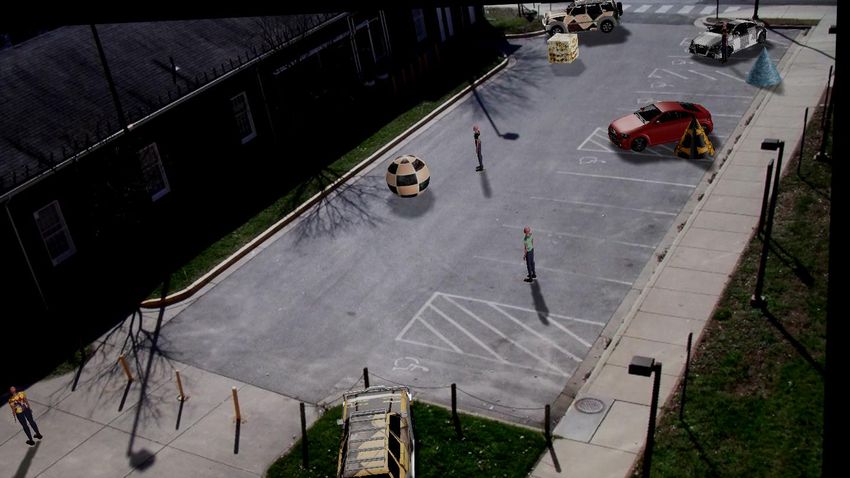
(a) Target domain
             (a) Target domain: sphere images

                                                                                          (b) Source domain

     (b) Source domain: sphere, cube, cylinder images                  Figure 6. Image classification (12 classes) for Syn2Real.
     Figure 4. Image classification (6 classes) for CLEVR.
                                                                      Results: We compare the target classification accuracy of
                                                                   DR, ADR and ADR+DA with the number of training images
   ADR Setup: The policy πω consists of |color|×|shape|×           in Fig. 5. Please note that for ADR+DA, we independently
|material| × |size| = 252 parameters representing a multino-       generated 1000 unlabeled images from the target domain.
mial distribution over Θ, initialized as a uniform distribution.   ADR eventually learns to generate images containing an
The learner h is implemented as ResNet18 followed by a             object of small size (first and second column in Fig 4). On
fully connected layer for classification which is trained end-     the other hand, DR keeps on occasionally generating images
to-end. The domain classifier D is a small fully connected         with large objects, such images are easier for the learner to
network accepting 512 dimensional feature vector extracted         classify due to a large number of pixels corresponding to
from conv5 layer of ResNet18 as input.                             the color of object. Interestingly ADR + DA performs the
                                                                   best, the domain classifier learns to discriminate generated
                                                                   images on the basis of the shape being sphere or not. This
                                                                   encourages the policy πω to generate images with spheres
                                                                   (images similar to target domain).

                                                                   5.1.2   Syn2Real
                                                                   We use 1,907 3D models by [30] in Blender3D to build a
                                                                   simulator for Syn2Real image classification. In our experi-
                                                                   ment, we use the validation split of Syn2Real as the target
                                                                   domain. The split contains 55,388 real images from the Mi-
                                                                   crosoft COCO dataset [26] for 12 classes. The input space X
                                                                   consists of images with resolutions 384 × 216 and the output
                                                                   space Y are the 12 categories. Here θ ∈ Θ corresponds to
                                                                   [image class]. Other parameters like camera elevation, light-
Figure 5. Effect of data size on DR, ADR and ADR+DA, target        ing and object pose are randomly sampled after quantization.
classification accuracy on CLEVR averaged over 10 independent      Refer Fig. 6 for visualizations of target and source domain.
runs.                                                              There are a total of 152,397 possible values of simulation pa-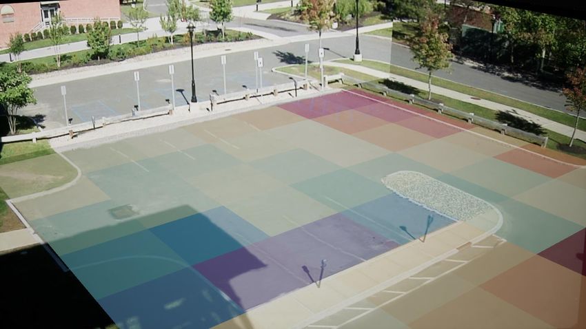
#Images 10k 25k 50k 100k All(150k)
DR 8.1 10.0 13.8 23.5 28.1 [30]
ADR 15.3 18.6 24.9 31.1 35.9
Table 1. Effect of data size on DR and ADR, target classification
accuracy for Syn2Real
rameters, each corresponds to an unique image in the source
domain.
ADR Setup: πω consists of |category of image| = 12 (a) Domain Randomization
parameters representing a multinomial distribution over Θ,
initialized as a uniform distribution. The learner h is AlexNet
[21] initialized with weights learned on ImageNet [9]. The
hyperparameters are similar to [30].
Results: Table 1 compares target classification of DR
and ADR with varying data size. We observe that ADR
focuses on confusing classes like (1) car and bus, (2) bike
and motorbike by trading off samples for easier classes like
plant and train. Note, we also include the case when every
possible image variation (152,397) is used to train the learner
h (All-150k). In this case, ADR reduces to hard negative
(b) Adversarial Domain Randomization
mining over image classes which performs better than the
baseline (Source) [30]. Figure 7. A comparison of source data for VIRAT from DR and
We also study the effect of ADR with unlabeled target ADR along with ground truth instance segmentation map.
data and various DA methods like ADA [50], Deep-CORAL
[43], DAN [27], SE [12] with same setup as [30] except for
ADA, we use a domain classifier with ResNet18 architecture. decides which object is placed where in the scene. To include
Refer Table 2 for per class performance of ADR-150k with variable number of objects in the image, we randomly sample
various DA methods. Note, we use all the target images n = number of objects (2 ≤ n ≤ 12) and invoke πω n times.
without labels for adaptation. Other parameters like lighting, texture, car model, pose, size
of the object are randomly sampled. The reward for policy
5.2. Object Detection πω is computed per cell and is negative of the IoU of the
bounding box predicted by the learner h.
We use the Unreal Engine 4 based simulator by [20] for The learner h is implemented as Faster-RCNN [34] with
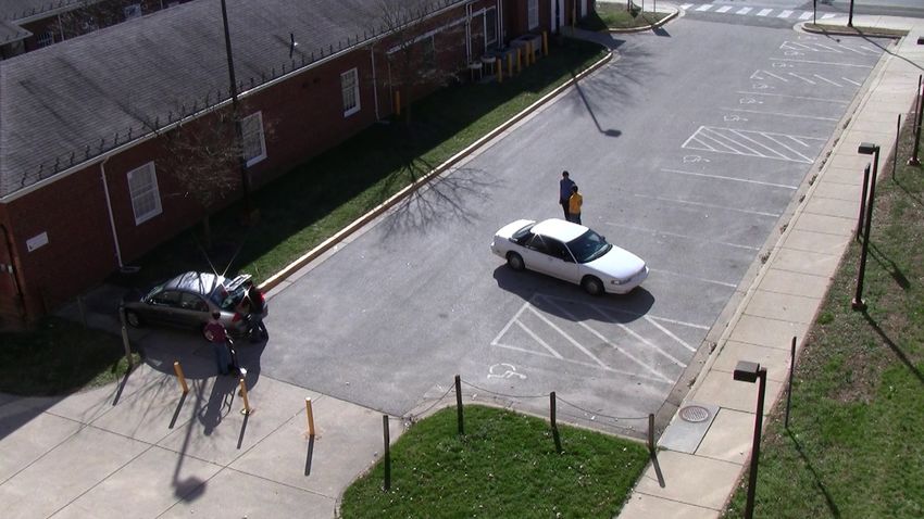
the VIRAT dataset [29]. VIRAT contains surveillance videos RoI-Align and ResNet101 with feature pyramid network
of parking lots. The simulator models the parking lot and [25] architecture as the backbone for all our evaluations.
the surveillance camera in a 3D world. The randomization
process uses a texture bank of 100 textures with 10 cars,
#Images 1k 10k 25k 50k 100k
5 person models and geometric distractors (cubes, cones,
spheres) along with varying lighting conditions, contrast and DR 20.6 32.1 43.7 54.9 75.8
brightness. In our experiment, we use 50,000 images from
two scenes of the dataset as the target domain. The input ADR 31.4 43.8 56.0 78.2 88.6
space X consists of images with resolution 1920 × 1080 Table 3. Effect of data size on DR and ADR, Faster-RCNN’s AP at
and the output space Y is the space of car bounding boxes 0.7 IoU on VIRAT.
(atmost 20) present in the image. Here θ ∈ Θ is a list of
object attributes in the image. These attributes specify the Results: Table 3 compares performance of DR and ADR
location and type of the object in the image. Fig. 1, 7 shows on target data along with the size of synthetic data. ADR
labeled samples from source domain. outperforms DR consistently by generating informative sam-
ADR Setup: We divide the scene ground plane into 45 ples for object detection containing object occlusions and
rectangular cells (refer Fig. 8). In each cell, we place three truncations. We compare data samples generated by DR and
kinds of objects (car, person or distractor). The policy πω ADR in Fig. 1, 7 along with a visualization of πω learned by
consists of |cells| × |types of objects| = 135 parameters ADR in Fig. 8, πω is shown as a heat-map (warmer colors
representing the object spawn probability i.e. the policy πω indicate higher object spawn probability). ADR learns to
DA Method          aero    bike   bus   car   horse   knife    mbke   prsn                   plant        skbrd                            train              truck                 mean
               All Source [30]     53      3     50    52     27      14       27     3                      26           10                               64                  4                   28.1
               ADA                 68      41    63    34     57      45       74     30                     57           24                               63                  15                  47.6
               D-CORAL [30]        76      31    60    35     45      48       55     28                     56           28                               60                  19                  45.5
               DAN [30]            71      47    67    31     61      49       72     36                     64           28                               70                  19                  51.6
               SE [30]             97      87    84    64     95      96       92     82                     96           92                               87                  54                  85.5
               ADR                 49      12    52    56     38      25       31     14                     34           32                               59                  29                  35.9
               ADA + ADR           73      50    60    38     59      51       79     37                     60           41                               69                  35                  54.3
               D-CORAL + ADR       78      56    71    48     64      59       77     45                     68           49                               70                  55                  61.6
               DAN + ADR           87      60    73    40     59      56       68     43                     72           39                               68                  51                  59.7
               SE + ADR            94      85    88    72     89      93       91     88                     93           86                               84                  75                  86.4
               Real [30]           94      83    83    86     93      91       90     86                     94           88                               87                  65                  87.2

                                     Table 2. Effect of unlabeled target data with ADR on Syn2Real

                                                                                                                                                                  car 0.99

                                                                                                 car 0.95

                                                                                                                                               car 0.97

                                                                                                                                    car 0.97
                                                                                                              car 0.99
                                                                                                                         car 0.88

                                                                                                 car 0.99

                                                                                                                                                                             car 0.99
                                                                                      car 1.00

                                                                                                                                                                                                          car 0.99

                                                                                                                                                  car 0.98

                                                                                                                         car 0.96

                                                                                                                                                                                        car 0.98

Figure 8. Object spawn probability (πω ) visualized as a heat-map.           Figure 9. Faster-RCNN trained on 100k images generated by ADR
The warmer colors indicate higher probability which correspond to
small/truncated/occluded objects in the image.
                                                                             on target images from VIRAT (Real). Using unlabeled data
              Method                     AP @ 0.7                            with synthetic data boosts performance from (for DR 75.8 to
              COCO                         80.2                              84.7, for ADR 88.6 to 93.6). However, the combination of
              ADA                          84.7                              labeled synthetic data and unlabeled real data still performs
              ADR-100k + ADA               93.6                              worse than labeled real data. We provide more analysis in
              Real                         98.1                              supplementary material.
Table 4. Effect of unlabeled target data with ADR on VIRAT.
                                                                             6. Conclusion
                                                                                DR is a powerful method that bridges the gap between
place objects far from the camera, thus making them diffi-                   real and synthetic data. There is a need to analyze such an
cult for the learner to detect. Fig. 9 shows examples of car                 important technique, our work is the first step in this direc-
detection from Faster-RCNN trained on data generated by                      tion. We theoretically show that DR is superior to synthetic
ADR, affirming that our method performs well under severe                    data generation without randomization. We also identify
truncations and occlusions.                                                  DR’s requirement of a lot of data for generalization. As an
   We also evaluate ADR with 5,000 unlabeled target images                   alternative, we proposed ADR, which generates adversarial
(not in the test set). Refer Table 4 for comparison of (1)                   samples with respect to the learner during training. Our eval-
Faster-RCNN trained on Microsoft-COCO dataset (COCO),                        uations show that ADR outperforms DR using less data for
(2) ADA [50] with ResNet18 as domain classifier, (3) ADR +                   image classification and object detection on real datasets.
ADA with 100k source images and (4) Faster-RCNN trained
References                                                             [17] J. Hoffman, D. Wang, F. Yu, and T. Darrell. Fcns in the wild:
                                                                            Pixel-level adversarial and constraint-based adaptation. arXiv
 [1] S. L. Arlinghaus and S. Arlinghaus. Google earth: Bench-               preprint arXiv:1612.02649, 2016. 2
     marking a map of walter christaller. 2007. 2                      [18] S. James, A. J. Davison, and E. Johns. Transferring end-to-
 [2] S. Ben-David, J. Blitzer, K. Crammer, A. Kulesza, F. Pereira,          end visuomotor control from simulation to real world for a
     and J. W. Vaughan. A theory of learning from different do-             multi-stage task. arXiv preprint arXiv:1707.02267, 2017. 2
     mains. Machine learning, 79(1-2):151–175, 2010. 3                 [19] J. Johnson, B. Hariharan, L. van der Maaten, L. Fei-Fei,
 [3] S. Ben-David, J. Blitzer, K. Crammer, and F. Pereira. Analysis         C. L. Zitnick, and R. Girshick. Clevr: A diagnostic dataset
     of representations for domain adaptation. In Advances in               for compositional language and elementary visual reasoning.
     neural information processing systems, pages 137–144, 2007.            In Computer Vision and Pattern Recognition (CVPR), 2017
     3                                                                      IEEE Conference on, pages 1988–1997. IEEE, 2017. 2, 5
 [4] K. Bousmalis, G. Trigeorgis, N. Silberman, D. Krishnan,           [20] R. Khirodkar, D. Yoo, and K. M. Kitani. Domain random-
     and D. Erhan. Domain separation networks. In Advances                  ization for scene-specific car detection and pose estimation.
     in Neural Information Processing Systems, pages 343–351,               arXiv preprint arXiv:1811.05939, 2018. 1, 2, 7
     2016. 2                                                           [21] A. Krizhevsky, I. Sutskever, and G. E. Hinton. Imagenet
 [5] G. Brockman, V. Cheung, L. Pettersson, J. Schneider, J. Schul-         classification with deep convolutional neural networks. In
     man, J. Tang, and W. Zaremba. Openai gym.(2016). arxiv.                Advances in neural information processing systems, pages
     arXiv preprint arXiv:1606.01540, 2016. 2                               1097–1105, 2012. 7
 [6] A. X. Chang, T. Funkhouser, L. Guibas, P. Hanrahan,               [22] A. Kundu, Y. Li, and J. M. Rehg. 3d-rcnn: Instance-level 3d
     Q. Huang, Z. Li, S. Savarese, M. Savva, S. Song, H. Su,                object reconstruction via render-and-compare. In Proceedings
     et al. Shapenet: An information-rich 3d model repository.              of the IEEE Conference on Computer Vision and Pattern
     arXiv preprint arXiv:1512.03012, 2015. 2                               Recognition, pages 3559–3568, 2018. 2
 [7] Y. Chen, W. Li, C. Sakaridis, D. Dai, and L. Van Gool. Do-        [23] J. Liao and A. Berg. Sharpening jensen’s inequality. The
     main adaptive faster r-cnn for object detection in the wild. In        American Statistician, pages 1–4, 2018. 4
     Proceedings of the IEEE Conference on Computer Vision and         [24] J. J. Lim, H. Pirsiavash, and A. Torralba. Parsing ikea objects:
     Pattern Recognition, pages 3339–3348, 2018. 2                          Fine pose estimation. In Proceedings of the IEEE Interna-
 [8] Y. Chen, W. Li, and L. Van Gool. Road: Reality oriented                tional Conference on Computer Vision, pages 2992–2999,
     adaptation for semantic segmentation of urban scenes. In               2013. 2
     Proceedings of the IEEE Conference on Computer Vision and         [25] T.-Y. Lin, P. Dollár, R. B. Girshick, K. He, B. Hariharan, and
     Pattern Recognition, pages 7892–7901, 2018. 2                          S. J. Belongie. Feature pyramid networks for object detection.
 [9] J. Deng, W. Dong, R. Socher, L.-J. Li, K. Li, and L. Fei-Fei.          In CVPR, volume 1, page 4, 2017. 7
     ImageNet: A Large-Scale Hierarchical Image Database. In           [26] T.-Y. Lin, M. Maire, S. Belongie, J. Hays, P. Perona, D. Ra-
     CVPR09, 2009. 7                                                        manan, P. Dollár, and C. L. Zitnick. Microsoft coco: Common
                                                                            objects in context. In European conference on computer vi-
[10] A. Dosovitskiy and V. Koltun. Learning to act by predicting
                                                                            sion, pages 740–755. Springer, 2014. 6
     the future. arXiv preprint arXiv:1611.01779, 2016. 2
                                                                       [27] M. Long, Y. Cao, J. Wang, and M. I. Jordan. Learning transfer-
[11] A. Dosovitskiy, G. Ros, F. Codevilla, A. Lopez, and V. Koltun.
                                                                            able features with deep adaptation networks. arXiv preprint
     Carla: An open urban driving simulator. arXiv preprint
                                                                            arXiv:1502.02791, 2015. 2, 7
     arXiv:1711.03938, 2017. 2
                                                                       [28] Z. Murez, S. Kolouri, D. Kriegman, R. Ramamoorthi, and
[12] G. French, M. Mackiewicz, and M. Fisher. Self-ensembling
                                                                            K. Kim. Image to image translation for domain adaptation.
     for domain adaptation. arXiv preprint arXiv:1706.05208,
                                                                            arXiv preprint arXiv:1712.00479, 13, 2017. 2
     2017. 7
                                                                       [29] S. Oh, A. Hoogs, A. Perera, N. Cuntoor, C.-C. Chen, J. T.
[13] Y. Ganin and V. Lempitsky. Unsupervised domain adaptation              Lee, S. Mukherjee, J. Aggarwal, H. Lee, L. Davis, E. Swears,
     by backpropagation. arXiv preprint arXiv:1409.7495, 2014.              X. Wang, Q. Ji, K. Reddy, M. Shah, C. Vondrick, H. Pirsi-
     2                                                                      avash, D. Ramanan, J. Yuen, A. Torralba, B. Song, A. Fong,
[14] Y. Ganin, E. Ustinova, H. Ajakan, P. Germain, H. Larochelle,           A. Roy-Chowdhury, and M. Desai. A large-scale benchmark
     F. Laviolette, M. Marchand, and V. Lempitsky. Domain-                  dataset for event recognition in surveillance video. IEEE
     adversarial training of neural networks. The Journal of Ma-            Comptuer Vision and Pattern Recognition (CVPR), 2011. 2,
     chine Learning Research, 17(1):2096–2030, 2016. 2                      5, 7
[15] H. Hattori, N. Lee, V. N. Boddeti, F. Beainy, K. M. Kitani, and   [30] X. Peng, B. Usman, K. Saito, N. Kaushik, J. Hoffman, and
     T. Kanade. Synthesizing a scene-specific pedestrian detector           K. Saenko. Syn2real: A new benchmark forsynthetic-to-real
     and pose estimator for static video surveillance. International        visual domain adaptation. arXiv preprint arXiv:1806.09755,
     Journal of Computer Vision, 2018. 2                                    2018. 2, 5, 6, 7, 8
[16] J. Hoffman, E. Tzeng, T. Park, J.-Y. Zhu, P. Isola, K. Saenko,    [31] X. B. Peng, M. Andrychowicz, W. Zaremba, and P. Abbeel.
     A. A. Efros, and T. Darrell. Cycada: Cycle-consistent adver-           Sim-to-real transfer of robotic control with dynamics random-
     sarial domain adaptation. arXiv preprint arXiv:1711.03213,             ization. In 2018 IEEE International Conference on Robotics
     2017. 2                                                                and Automation (ICRA), pages 1–8. IEEE, 2018. 2
[32] L. Pinto, M. Andrychowicz, P. Welinder, W. Zaremba, and            [47] Y. Tassa, Y. Doron, A. Muldal, T. Erez, Y. Li, D. d. L. Casas,
     P. Abbeel. Asymmetric actor critic for image-based robot                D. Budden, A. Abdolmaleki, J. Merel, A. Lefrancq, et al.
     learning. arXiv preprint arXiv:1710.06542, 2017. 2                      Deepmind control suite. arXiv preprint arXiv:1801.00690,
[33] A. Prakash, S. Boochoon, M. Brophy, D. Acuna, E. Cam-                   2018. 2
     eracci, G. State, O. Shapira, and S. Birchfield. Structured        [48] J. Tobin, R. Fong, A. Ray, J. Schneider, W. Zaremba, and
     domain randomization: Bridging the reality gap by context-              P. Abbeel. Domain randomization for transferring deep neural
     aware synthetic data. arXiv preprint arXiv:1810.10093, 2018.            networks from simulation to the real world. In Intelligent
     3                                                                       Robots and Systems (IROS), 2017 IEEE/RSJ International
[34] S. Ren, K. He, R. Girshick, and J. Sun. Faster r-cnn: Towards           Conference on, pages 23–30. IEEE, 2017. 1, 2
     real-time object detection with region proposal networks. In       [49] J. Tremblay, A. Prakash, D. Acuna, M. Brophy, V. Jampani,
     Advances in neural information processing systems, pages                C. Anil, T. To, E. Cameracci, S. Boochoon, and S. Birch-
     91–99, 2015. 7                                                          field. Training deep networks with synthetic data: Bridging
[35] S. R. Richter, Z. Hayder, and V. Koltun. Playing for bench-             the reality gap by domain randomization. arXiv preprint
     marks. In International conference on computer vision                   arXiv:1804.06516, 2018. 1, 2
     (ICCV), volume 2, 2017. 2                                          [50] E. Tzeng, J. Hoffman, K. Saenko, and T. Darrell. Adversarial
                                                                             discriminative domain adaptation. In Computer Vision and
[36] S. R. Richter, V. Vineet, S. Roth, and V. Koltun. Playing
                                                                             Pattern Recognition (CVPR), volume 1, page 4, 2017. 2, 5, 7,
     for data: Ground truth from computer games. In European
                                                                             8
     Conference on Computer Vision, pages 102–118. Springer,
     2016. 2                                                            [51] E. Tzeng, J. Hoffman, N. Zhang, K. Saenko, and T. Darrell.
                                                                             Deep domain confusion: Maximizing for domain invariance.
[37] G. Ros, L. Sellart, J. Materzynska, D. Vazquez, and A. M.
                                                                             arXiv preprint arXiv:1412.3474, 2014. 2
     Lopez. The synthia dataset: A large collection of synthetic
     images for semantic segmentation of urban scenes. In Pro-          [52] G. Varol, J. Romero, X. Martin, N. Mahmood, M. J. Black,
     ceedings of the IEEE conference on computer vision and                  I. Laptev, and C. Schmid. Learning from synthetic humans.
     pattern recognition, pages 3234–3243, 2016. 2                           In 2017 IEEE Conference on Computer Vision and Pattern
                                                                             Recognition (CVPR 2017), pages 4627–4635. IEEE, 2017. 2
[38] F. Sadeghi and S. Levine. Cad2rl: Real single-image flight
                                                                        [53] M. Wang and W. Deng. Deep visual domain adaptation: A
     without a single real image. arXiv preprint arXiv:1611.04201,
                                                                             survey. Neurocomputing, 2018. 1
     2016. 2
                                                                        [54] R. J. Williams. Simple statistical gradient-following algo-
[39] F. S. Saleh, M. S. Aliakbarian, M. Salzmann, L. Petersson,
                                                                             rithms for connectionist reinforcement learning. Machine
     and J. M. Alvarez. Effective use of synthetic data for urban
                                                                             learning, 8(3-4):229–256, 1992. 5
     scene semantic segmentation. In European Conference on
                                                                        [55] Y. Xiang, W. Kim, W. Chen, J. Ji, C. Choy, H. Su, R. Mot-
     Computer Vision, pages 86–103. Springer, Cham, 2018. 2
                                                                             taghi, L. Guibas, and S. Savarese. Objectnet3d: A large scale
[40] R. J. Serfling. Probability inequalities for the sum in sampling        database for 3d object recognition. In European Conference
     without replacement. The Annals of Statistics, pages 39–48,             on Computer Vision, pages 160–176. Springer, 2016. 2
     1974. 3
                                                                        [56] Y. Xiang, R. Mottaghi, and S. Savarese. Beyond pascal: A
[41] S. Shah, D. Dey, C. Lovett, and A. Kapoor. Airsim: High-                benchmark for 3d object detection in the wild. In Applications
     fidelity visual and physical simulation for autonomous vehi-            of Computer Vision (WACV), 2014 IEEE Winter Conference
     cles. In Field and Service Robotics, 2017. 2                            on, pages 75–82. IEEE, 2014. 2
[42] H. Su, C. R. Qi, Y. Li, and L. J. Guibas. Render for cnn:          [57] Y. Zhang, P. David, and B. Gong. Curriculum domain adap-
     Viewpoint estimation in images using cnns trained with ren-             tation for semantic segmentation of urban scenes. In The
     dered 3d model views. In The IEEE International Conference              IEEE International Conference on Computer Vision (ICCV),
     on Computer Vision (ICCV), December 2015. 2                             volume 2, page 6, 2017. 2
[43] B. Sun, J. Feng, and K. Saenko. Return of frustratingly easy
     domain adaptation. In Thirtieth AAAI Conference on Artificial
     Intelligence, 2016. 7
[44] M. Sundermeyer, Z. Marton, M. Durner, and R. Triebel. Im-
     plicit 3d orientation learning for 6d object detection from
     rgb images. In Proceedings of the European Conference on
     Computer Vision (ECCV), pages 699–715, 2018. 2
[45] R. S. Sutton, D. A. McAllester, S. P. Singh, and Y. Man-
     sour. Policy gradient methods for reinforcement learning with
     function approximation. In Advances in neural information
     processing systems, pages 1057–1063, 2000. 5
[46] J. Tan, T. Zhang, E. Coumans, A. Iscen, Y. Bai, D. Hafner,
     S. Bohez, and V. Vanhoucke. Sim-to-real: Learning
     agile locomotion for quadruped robots. arXiv preprint
     arXiv:1804.10332, 2018. 2
You can also read