SelfReg: Self-supervised Contrastive Regularization for Domain Generalization
←
→
Page content transcription
If your browser does not render page correctly, please read the page content below
SelfReg: Self-supervised Contrastive Regularization for Domain Generalization

                                                                 Daehee Kim1 , Seunghyun Park2 , Jinkyu Kim3 , and Jaekoo Lee1
                                                                                  1
                                                                                      College of Computer Science, Kookmin University
                                                                                            2
                                                                                                Clova AI Research, NAVER Corp.
                                                                        3
                                                                            Department of Computer Science and Engineering, Korea University
arXiv:2104.09841v1 [cs.CV] 20 Apr 2021

                                                                 Abstract

                                             In general, an experimental environment for deep learn-
                                         ing assumes that the training and the test dataset are sam-
                                         pled from the same distribution. However, in real-world
                                         situations, a difference in the distribution between two
                                         datasets, domain shift, may occur, which becomes a ma-
                                         jor factor impeding the generalization performance of the                                                        SelfReg

                                         model. The research field to solve this problem is called                      : Inter-domain Self-supervised Dissimilarity Loss
                                         domain generalization, and it alleviates the domain shift                            : Domains                : Classes

                                         problem by extracting domain-invariant features explicitly
                                         or implicitly. In recent studies, contrastive learning-based            Figure 1. Our model utilizes the self-supervised contrastive losses
                                         domain generalization approaches have been proposed and                 for the model to learn domain-invariant representation by mapping
                                         achieved high performance. These approaches require sam-                the latent representation of the same-class samples close together.
                                         pling of the negative data pair. However, the performance of            Note that different shapes (i.e. circles, stars, and squares) indicate
                                         contrastive learning fundamentally depends on quality and               different classes Ci∈{1,2,3} , and we differently color-code accord-
                                         quantity of negative data pairs. To address this issue, we              ing to their domain Di∈{1,2,3,4} .
                                         propose a new regularization method for domain general-
                                         ization based on contrastive learning, self-supervised con-
                                                                                                                 often domain-invariant to low-level visual cues [35], some
                                         trastive regularization (SelfReg). The proposed approach
                                                                                                                 studies [10] suggest that they are still susceptible to domain
                                         use only positive data pairs, thus it resolves various prob-
                                                                                                                 shift.
                                         lems caused by negative pair sampling. Moreover, we pro-
                                                                                                                     There have been increasing efforts to develop models
                                         pose a class-specific domain perturbation layer (CDPL),
                                                                                                                 that can generalize well to out-of-distribution. The litera-
                                         which makes it possible to effectively apply mixup augmen-
                                                                                                                 ture in domain generalization (DG) aims to learn the in-
                                         tation even when only positive data pairs are used. The ex-
                                                                                                                 variances across multiple different domains so that a clas-
                                         perimental results show that the techniques incorporated
                                                                                                                 sifier can robustly leverage such invariances in unseen test
                                         by SelfReg contributed to the performance in a compati-
                                                                                                                 domains [40, 15, 29, 28, 31, 38]. In the domain general-
                                         ble manner. In the recent benchmark, DomainBed, the pro-
                                                                                                                 ization task, it is assumed that multiple source domains
                                         posed method shows comparable performance to the con-
                                                                                                                 are accessible during training, but the target domains are
                                         ventional state-of-the-art alternatives. Codes are available
                                                                                                                 not [4, 31]. This is different from domain adaptation (DA),
                                         at https://github.com/dnap512/SelfReg.
                                                                                                                 semi-supervised domain adaptation (SSDA), and unsuper-
                                                                                                                 vised domain adaptation (UDA) problems, where examples
                                                                                                                 from the target domain are available during training. In this
                                         1. Introduction
                                                                                                                 paper, we focus on the domain generalization task.
                                            Machine learning systems often fail to generalize out-of-                Some recent studies [7, 20, 33] suggest that contrastive
                                         sample distribution as they assume that in-samples and out-             learning can be successfully used in a self-supervised learn-
                                         of-samples are independent and identically distributed – this           ing task by mapping the latent representations of the posi-
                                         assumption rarely holds during deployment in real-world                 tive pair samples close together, while that of negative pair
                                         scenarios where the data is highly likely to change over time           samples further away in the embedding space. Such a con-
                                         and space. Deep convolutional neural network features are               trastive learning strategy has also been utilized for the do-

                                                                                                             1
main generalization tasks [30, 11], similarly aiming to re-       nik et al. [40] introduces Empirical Risk Minimization
duce the distance of same-class features in the embedding         (ERM) that minimizes the sum of errors across domains.
space, while increasing the distance of different-class fea-      Notable variants have been introduced to learn domain-
tures. However, such negative pairs often make the training       invariant features by matching distributions across differ-
unstable unless useful negative samples are available in the      ent domains. Ganin et al. [15] utilizes an adversarial net-
same batch, which is but often challenging.                       work to match such distributions, while Li et al. [29] in-
    In this work, we revisit contrastive learning for the do-     stead matches the conditional distributions across domains.
main generalization task, but only with positive pair sam-        Such a shared feature space is optimized by minimizing
ples, as shown in Figure 1. As it is generally known that         maximum mean discrepancy [28], transformed feature dis-
using positive pair samples only causes the performance           tribution distance [31], or covariances [38]. In this work, we
drop, which is often called representation collapse [17]. In-     also follow this stream of work, but we explore the benefit
spired by recent studies on self-supervised learning [8, 17],     of self-supervised contrastive learning that can inherently
which successfully avoids representation collapse by plac-        learn to domain-invariant discriminating feature by explic-
ing one more projection layer at the end of the network, we       itly mapping the “same-class” latent representations close
successfully learn domain-invariant features and our model        together.
trained with self-supervised contrastive losses shows the             To our best knowledge, there are few that applied
matched or better performance against alternative state-of-       contrastive learning in the domain generalization set-
the-art methods, where ours is ranked at 2nd places in the        ting. Classification and contrastive semantic alignment
domain generalization benchmarks, i.e. DomainBed [18].            (CCSA) [30] and model-agnostic learning of semantic fea-
    However, self-supervised contrastive losses are only part     tures (MASF) [11] aimed to reduce the distance of same-
of the story. As we generally use a linear form of the loss       class (positive pair) feature distributions while increasing
function, properly balancing gradients is required so that        the distance of different-class (negative pair) feature distri-
network parameters converge to generate domain-invariant          butions. However, using such negative pairs often make the
features. To mitigate this issue, we advocate for applying        training unstable unless useful negative samples are avail-
the following three gradient stabilization techniques: (i) loss   able in the same batch, which is often challenging. To ad-
clipping, (ii) stochastic weights averaging (SWA), and (iii)      dress this issue, we focus on minimizing a distance between
inter-domain curriculum learning (IDCL). We observe that          the same-class (positive pair) features in the embedding
the combined use of these techniques further improves the         space as recently studied for the self-supervised learning
model’s generalization power.                                     task [7, 20, 33], including BYOL [17] and SimSiam [8].
    To effectively evaluate our proposed model, we first              Inter-domain mixup [45, 44, 43] techniques are intro-
use the publicly available domain generalization data set         duced to perform empirical risk minimization on linearly
called PACS [26], where we analyzed our model in detail           interpolated examples from random pairs across domains.
to support our claims. We further experiment with much            We also utilize such a mixup, but we only interpolate same-
larger benchmarks called DomainBed [18] where our model           class features to preserve the class-specific features. We ob-
shows matched or better performance against alternative           serve that such a same-class mixup help obtaining robust
state-of-the-art methods.                                         performance for unseen domain data.
    We summarize our main contributions as follows:                   As another branch, JiGen [5] utilizes a self-supervised
                                                                  signal by solving a jigsaw puzzle as a secondary task to
   • SelfReg facilitates the application of metric learning
                                                                  improve generalization. Meta-learning frameworks [27] are
     using only positive pairs without negative pairs.
                                                                  also explored for domain generalization to meta-learn how
   • We devised a CDPL by exploiting a condition that             to generalize across domains by leveraging MAML [14].
     use only positive pairs. The combination of CDPL and         Some also explored splitting the model into domain-
     mixup improves the weakness of mixup approach.               invariant and domain-variant components by low-rank pa-
   • The performance comparable to that of the SOTA DG            rameterization [26], style-agnostic network [32], domain-
     methods was confirmed in the DomainBed that facil-           specific aggregation modules [12].
     itated the comparison of DG performance in the fair
     and realistic environment.                                   3. Method

2. Related Work                                                      We start by motivating our method before explaining its
                                                                  details. The main goal of domain generalization is to learn
   The main goal of domain generalization (DG) is to gen-         a domain-invariant representation from multiple source do-
erate domain-invariant features so that the model is gener-       mains so that a model can generalize well across unseen
alizable to unseen target domains, which are generally out-       target domains. While domain-variant representation can be
side the training distribution. Of a landmark work, Vap-          achieved to some degree through deep network architec-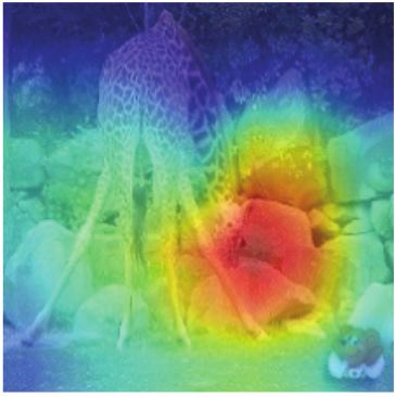
Inter-domain Curriculum Learning                               Test               Forward            Mixup
                                                                                                                      Shuffle            Distance

                                          Regularization         Regularization
                                             Block                  Block

                              (a) SelfReg Architecture                                                    (b) Regularization Block

Figure 2. An overview of our proposed SelfReg. Here, we propose to use the self-supervised (in-batch) contrastive losses to regularize the
model to learn domain-invariant representations. These losses regularize the model to map the representations of the “same-class” samples
close together in the embedding space. We compute the following two dissimilarities in the embedding space: (i) individualized and (ii)
heterogenerous self-supervised dissimilarity losses. We further use the stochastic weight average (SWA) technique and the inter-domain
curriculum learning (IDCL) to optimize gradients in conflict directions.

tures, invariant representations are often harder to achieve                  trastive losses and observe a further performance improve-
and are usually implicitly learned with the task. To address                  ment, which is possibly due to SWA provides the more flat-
this, we argue that a model should learn a domain-invariant                   ness in loss surface by ensembling domain-specific models.
discriminating feature by comparing among different sam-                      We exclude contents of the inter-domain curriculum learn-
ples – the comparison can be performed between positive                       ing (IDCL) strategy in this paper because of publication
pairs of same-class inputs and negative pairs of different-                   copyright issues.
class inputs.
                                                                              3.1. Individualized In-batch Dissimilarity Loss
    Here we propose the self-supervised contrastive losses
to regularize the model to learn domain-invariant represen-                        Given latent representations zci = fθ (xi ) for i ∈
tation by mapping the representations of the “same-class”                     {1, 2, . . . , N } and a class label c ∈ C, we compute the in-
samples close together, while that of “different-class” sam-                  dividualized in-batch dissimilarity loss Lind . Note that we
ples further away in the embedding space. This may share                      use a feature generator fθ parameterized by θ and we use a
a similar idea with contrastive learning, which trains a                      batch size of N . The dissimilarity between a positive pair
discriminative model on multiple input pairs according to                     of the “same-class” latent representations is measured as in
some notion of similarity. Thus, we start with the recent                     the following Eq. 1:
batch contrastive approaches and extend them to the do-
                                                                                                      N
main generalization setting, as shown in Figure 2. While                                           1 X c                             2
                                                                                                         zi − fCDPL zcj∈[1,N ]

some domain generalization approaches need to modify                                  Lind (z) =                                     2
                                                                                                                                              (1)
                                                                                                   N i=1
the model architecture during learning, our proposed con-
trastive method is much simpler where no modification to                      where zcj is randomly chosen from other in-batch latent rep-
the model architecture is needed.                                             resentations {zci } that has the same class label c ∈ C. Note
    In the next section, we explain our proposed self-                        that we only consider optimizing the alignment of positive
supervised contrastive losses for domain generalization                       pairs and the uniformity of the representation distribution at
tasks, which mainly measures the following two feature-                       the same time. As discussed in [17], we use an additional
level dissimilarities in the embedding space: (i) Individ-                    an MLP layer fCDPL , called Class-specific Domain Pertur-
ualized In-batch Dissimilarity Loss (Section 3.1) and (ii)                    bation Layer, to prevent the performance drop caused by
Heterogeneous In-batch Dissimilarity Loss (Section 3.2).                      so-called representation collapse. We provide an ablation
Note that these losses can be applied to both the intermedi-                  study in Section 4.4 to confirm the use of fCDPL achieves
ate features and the logits from the classifier (Section 3.3).                better performance.
In fact, in our ablation study (Section 4.4), the combined                       For better computational efficiency, we use the following
use of both regularization achieves the best performance. In                  two steps to find all positive pairs, as shown in Figure 3. (i)
Section 3.4, we also discuss the stochastic weight average                    We first cluster and order latent representations zi into a
(SWA) technique that we use with our self-supervised con-                     same-class group, i.e. {zci } for c ∈ C. (ii) For each same-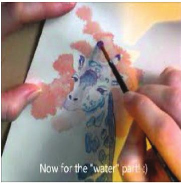
which often needs to be properly balanced so that network
                              ’    ’
                                                                    parameters converge to generate domain-invariant features
                                                                    that are also useful for the original classification task. We
                                  Shuffled
                                                                    observe that our self-supervised contrastive losses LSelfReg
                                                                    become dominant after the initial training stage, inducing
                              ’    ’         ’
                                                                    gradient imbalances to impede proper training. To miti-
                                                                    gate this issue, we apply two gradient stabilization tech-

                                                 Mixup
                                                                    niques: (i) loss clipping and (ii) stochastic weights aver-
                                                                    aging (SWA), and (iii) inter-domain curriculum learning
                                                                    (IDCL). For (i), we modify gradient magnitudes to be de-
                                                                    pendent on the magnitude of the classification loss Lc – i.e.
                                                                    we use the gradient magnitude modifier min(1.0, Lc ) and
                                                                    thus Lfeature = min(1.0, Lc ) γLind + (1 − γ)Lhdl . For (ii)
Figure 3. An overview of our proposed self-supervised contrastive
regularization losses.                                              we discuss details in Section 3.4.
                                                                    Loss Function Ultimately, we use the following loss func-
                                                                    tion L that consists of classification loss Lc as well as our
class group, we modify its order by random shuffling and
                                                                    self-supervised contrastive loss LSelfReg :
obtain SHUFFLE{zci }. (iii) We finally form a positive pair
in order from {zci } and SHUFFLE{zci }.                                                  L = Lc + LSelfReg                    (5)
3.2. Heterogeneous In-batch Dissimilarity Loss
                                                                    3.4. Stochastic Weights Averaging (SWA)
    To further push the model to learn domain-invariant
representations, we use an additional loss, called heteroge-            Stochastic Weight Average (SWA) is an ensembling
neous in-batch dissimilarity loss. Given latent representa-         technique to find a flatter minimum in loss space by aver-
tions ui = fCDPL (zci ) from the previous step, we apply a          aging snapshots of model parameters derived from multi-
two-domain Mix-up layer to obtain the interpolated latent           ple local minima in the training procedure [23]. It is known
representation z̄i across different domains. This regularizes       that finding a flatter minima guarantees better generaliza-
the model on the mixup distribution [46], i.e. a convex com-        tion performance [19], and thus it has been used in domain
bination of samples from different domains. This is similar         adaptation and generalization fields that require high gener-
to a layer proposed by Wang et al. [43] as defined as fol-          alization performance [48, 6].
lows:                                                                   Given model weight space Ω = {ω0 , ω1 , . . . , ωN },
               ūci = γuci + (1 − γ)ucj∈[1,N ]            (2)       where N is the number of training steps. There is no spe-
                                                                    cific constraint for sampling model weights, however, in
where γ ∼ Beta(α, β) for α = β ∈ (0, ∞). Similarly, ucj             general, sampling process is performed at a specific pe-
is randomly chosen from {uci } for i ∈ {1, 2, . . . , N } that      riod while the model is sufficiently converged. We use c as
have the same class label. Note that γ ∈ [0, 1] is controlled       a cyclic step length and sample weight space for SWA is
by hyper-parameters α and β.                                        Ωswa = {ωm+kc } for k ≥ 0, 0 ≤ m ≤ m + kc ≤ N , where
    Finally, we compute the heterogeneous in-batch dissim-          m indicates the initial step for SWA. Then we can derive the
ilarity loss Lhdl (z) as follows:                                   averaged weight wswa as follows:
                               N
                            1 X c                        2                                           k
               Lhdl (z) =         z − ūci                   (3)                                1 X
                            N i=1 i                      2                           ωswa =             ωm+ic .               (6)
                                                                                              k + 1 i=0
3.3. Feature and Logit-level Self-supervised Con-
      trastive Losses                                               Note that we use SWA to examine whether the proposed
                                                                    method is compatible with other existing techniques. There-
     The proposed individualized and heterogeneous in-              fore, we apply SWA only for ablation study (Section 4.4),
batch dissimilarity losses can be applied to both the inter-        not DomainBed (Section 5), for a fair comparison.
mediate features and the logits from the classifier. We use
the loss function LSelfReg as follows:                              4. Proof-of-Concept Experiments
            LSelfReg = λfeature Lfeature + λlogit Llogit     (4)    4.1. Implementation and Evaluation Details
where we use λfeature and λlogit to control the strength of            Following Huang et al. [22], we train our model, for
each term. As we use a linear form of the loss function,            approximately 30 epochs, with a SGD optimizer using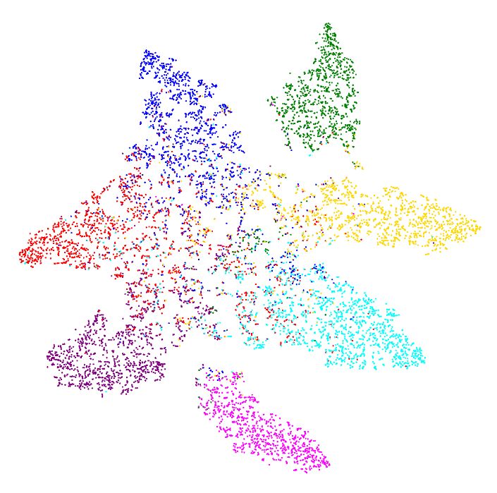
Dog                                            Dog                                                   Dog
                                          Elephant                                       Elephant                                              Elephant
                                          Giraffe                                        Giraffe                                               Giraffe
                                          Guitar                                         Guitar                                                Guitar
                                          Horse                                          Horse                                                 Horse
                                          House                                          House                                                 House
                                          Person                                         Person                                                Person

                  (a) Baseline                                     (b) RSC                                             (c) SelfReg (ours)

Figure 4. Visualizations by t-SNE [39] for (a) baseline (no DG techniques), (b) RSC [22], and (c) ours. For better understanding, we also
provide sample images of house from all target domains. Note that we differently color-coded each points according to its class. Data:
PACS [26]

ResNet18 [21] as a backbone, which is pretrained on Im-                Table 1. Image recognition accuracy (%) comparison with the
                                                                       state-of-the-art approach, RSC [22], on PACS [26] test set. We
ageNet [9]. Our backbone produces 512-dimensional latent
                                                                       also report standard deviation from a set of 20 models individually
representation from the last layer. The batch size is set to
                                                                       trained for each model and each test domain.
128 and learning rate to 0.004, which is decayed to 0.1 at
24 epochs. Note that such a decaying learning rate is not                                                     Test Domain
                                                                       Model                                                                   Average
used when it combined with the Stochastic Weights Aver-                                       Photo     Art Painting    Cartoon     Sketch
aging technique, where we instead compute the averaged
                                                                       A. DeepAll           95.66 ± 0.4 79.89 ± 1.3 75.61 ± 1.5 73.33 ± 2.8 81.12 ± 0.8
weight wswa at the every end of each epoch.                            B. RSC [22]          94.56 ± 0.4 79.88 ± 1.7 76.87 ± 1.2 77.11 ± 2.7 82.10 ± 0.9

                                                                       C. A + SelfReg (ours) 96.22 ± 0.3 82.34 ± 0.5 78.43 ± 0.7 77.47 ± 0.8 83.62 ± 0.3
   The loss weights are λfeature = 0.3 and λlogit = 1.0 were
determined using grid-search. For a two-domain Mix-up
layer, we use α = β = 0.5. The model architecture for the
class-specific domain perturbation layer fCDPL is a 2-layer            4.2. Performance Evaluation
MLPs with the number of hidden units set to 1024, where
                                                                           In Table 1, we first compare our model with the state-
we apply batch normalization followed by ReLU activation
                                                                       of-the-art method, called Representation Self-Challenging
function. Following RSC [22], data augmentation is used in
                                                                       (RSC) [22], which iteratively discards the dominant features
our experiments to improve model generalizability. This is
                                                                       during training and thus encourages the network to fully use
done by randomly cropping, flipping horizontally, jittering
                                                                       remaining features for the final verdict. For a fair compar-
color, and changing the intensity.
                                                                       ison, all models use the identical backbone ConvNet, i.e.
                                                                       ResNet18. To see the performance variance, we trained each
                                                                       model 20 times for each test domain and report the average
Dataset To verify the effectiveness of the proposed method,
                                                                       image recognition accuracy and its standard deviation. As
we evaluate our proposed method on the publicly available
                                                                       shown in Table 1, our proposed model clearly outperforms
PACS [26]. This benchmark dataset contains the overall 10k
                                                                       the other approaches in all test domains (compare the model
images from four different domains: P hoto, Art P ainting,
                                                                       B vs. model C), and the average image recognition accuracy
Cartoon, and Sketch. This dataset is particularly useful
                                                                       is 1.52% better than RSC [28], while produces lower model
in domain generalization research as it provides a bigger
                                                                       variance (0.9 vs. 0.3 on average).
domain shift than existing photo-only benchmarks. This
dataset provides seven object categories: i.e. dog, elephant,          Qualitative Analysis by t-SNE We use t-SNE [39] to com-
giraffe, guitar, horse, house, and person. We follow the               pute pairwise similarities in the latent space and visualize
same train-test split strategy from [26], we split exam-               in a low dimensional space by matching the distributions
ples from training domains to 9:1 (train:val) and test on              by KL divergence. In Figure 4, we provide a comparison of
the whole held-out domain. Note that we use the best-                  t-SNE visualizations of baseline, RSC, and ours. The bet-
performed model on validation for testing.                             ter a model generalizes well, the points in the t-SNE should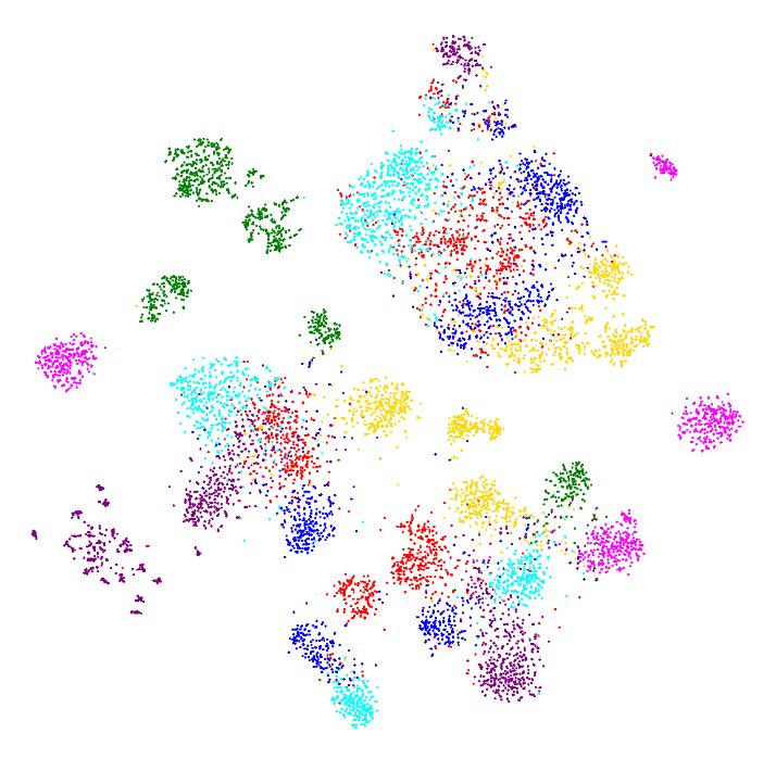
Target domain
be more clustered. As shown in Figure 4, (a) the baseline
Photo Art Painting Cartoon Sketch
model and (b) RSC [22] produce scattered multiple clus-
ters for each domain and class (see houses in the different
Input image
clusters according to their domain). Ours is not the case for
this. As shown in Figure 4 (c), objects from the same class
tend to form a merged cluster, making latent representations
close to each other in the high-dimensional space.
SelfReg (ours)
(a)
Euclidean distance
Feature-level
pairwise
RSC
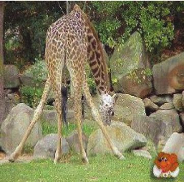
Epochs Figure 6. Original images with a giraffe for different domains
(b) (1st row). We provide visualizations of Grad-CAM [37] for ours
and RSC [22] , which localizes class-discriminative regions. Data:
Euclidean distance
PACS [26]
Logit-level
pairwise
amples from a single source domain (not multiple source
domains as we see in a previous experimental setting), and
then we evaluate with examples from other remaining tar-
get domains. As shown in Table 2, we report scores for
Epochs all source-target combinations, i.e. rows and columns for
source and target domains, respectively. As a baseline, we
Figure 5. Distance between (a) a pair of same-class features and compare ours with those of RSC [22] evaluated in the same
(b) a pair of same-class logits. We measure such distance at every setting (compare scores in left and right tables). We also re-
epoch during training and compare ours (solid red) with baseline port their differences in the last row (‘+’ indicates that ours
(dotted). Euclidean-based distance is used to measure distance in performs better). We observe in Table 2 that ours generally
feature space. Data: PACS [26] outperform alternative, where the average accuracy is im-
proved by 0.93%.
The Effect of Dissimilarity Loss We propose two types of
self-supervised contrastive loss that map the ”same-class” 4.4. Ablation Study
samples close together. We observe in Figure 5 that ”same-
class” pairwise distance is effectively regularized in both In Table 3, we compare variants of our model by remov-
latent (a) feature and (b) logit space (compare dotted (base- ing each component: i.e. (i) feature-level in-batch dissim-
line) vs. red solid line (ours)). This was not the case for ilarity regularization, (ii) logit-level in-batch dissimilarity
the baseline. Note that we use Euclidean-based distance to regularization, (iii) a two-domain mix-up layer, (iv) a class-
measure the pairwise difference. specific domain perturbation layer (CDPL), (v) stochastic
weights averaging (SWA), and (vi) inter-domain curriculum
Analysis with GradCAM We use GradCAM [37] to visu- learning (IDCL).
alize image regions where the network attends to. In Fig. 6,
we provide examples for different target domains where we Effect of Inter-domain Curriculum Learning (IDCL)
compare the model’s attention maps. We observe ours bet- We observe in Table 3 that applying our inter-domain cur-
ter captures the class-invariant feature (i.e. the long neck of riculum learning (IDCL) provides the recognition accuracy
the giraffe), while RSC [22] does not. Red is the attended (compare model A vs. B). Scores are generally improved in
region for the network’s final verdict. all target domains, i.e. the average accuracy is improved by
0.32%.
4.3. Single-source Domain Generalization
Effect of Stochastic Weights Averaging (SWA) As shown
We also evaluate our model in an extreme case for the in Table 3, the use of stochastic weight average technique
domain generalization task. We train our model with ex- further provides better performance (compare model B vs.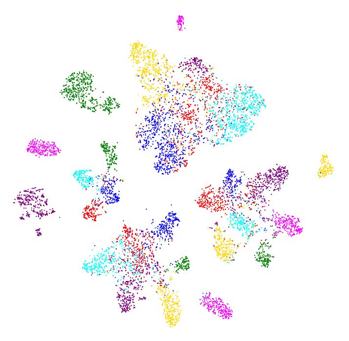
Table 2. As an extreme case for the domain generalization task, we train our model with a single source domain (rows) and evaluate with
other remaining target domains (columns). As a baseline, we also compare with RSC [22] of the same setting (compare left and right
tables). We also report their differences in the last row (+ indicates that ours performs better).

                                          Target domain                                                                        Target domain
RSC [22]                                                                             SelfReg
               Photo       Art Painting     Cartoon         Sketch     Average                     Photo        Art Painting      Cartoon        Sketch         Average

Photo             -        66.33 ± 1.8 26.47± 2.5 32.08 ± 2.0 41.63 ± 1.6 Photo                      -          67.72 ± 0.7     28.97 ± 1.0    33.71 ± 2.6     43.46 ± 1.1
Art Painting 96.28 ± 0.4        -          62.54 ± 2.1 53.19 ± 3.2 70.67 ± 1.2 Art Painting     96.62 ± 0.3          -          65.22 ± 0.7    55.94 ± 3.1     72.59 ± 1.1
Cartoon      85.89 ± 1.1 68.99 ± 1.4            -         70.38 ± 1.7 75.08 ± 1.0 Cartoon       87.53 ± 0.8     72.09 ± 1.2          -         70.06 ± 1.6     76.56 ± 0.8
Sketch       47.40 ± 3.5 37.99 ± 1.4 56.36 ± 3.0              -      47.25 ± 2.9 Sketch         46.07 ± 5.3     37.17 ± 4.0     54.03 ± 3.2         -          45.76 ± 3.8

Average        76.52          57.77           48.45         51.88       58.66        Average   76.74 (+0.22%) 58.99 (+1.22%) 49.41 (+0.96%) 53.24 (+1.36%) 59.59 (+0.93%)

Table 3. Ablation study of SelfReg on PACS. Abbr. Rf : feature-level in-batch dissimilarity loss, Rl : logit-level in-batch dissimilarity
loss, Mix-up: two-domain mix-up layer, CDPL: class-specific domain perturbation layer, SWA: stochastic weights averaging, IDCL: inter-
domain curriculum learning
                                                            Components                                               Test Domain
    Model                                                                                                                                                    Average
                                      Llogit Lfeature Mixup CDPL SWA IDCL                        Photo        Art Painting     Cartoon         Sketch

    A. SelfReg (Ours)                  X            X        X        X          X        X    96.22 ± 0.3 82.34 ± 0.5 78.43 ± 0.7 77.47 ± 0.8 83.62 ± 0.3

    B. A w/o IDCL                      X            X        X        X          X             96.09 ± 0.3 81.89 ± 0.6 78.03 ± 0.4 77.21 ± 1.1 83.30 ± 0.3
    C. B w/o SWA                       X            X        X        X                        96.10 ± 0.5 81.43 ± 1.0 77.86 ± 1.0 76.81 ± 1.2 83.05 ± 0.5
    D. C w/o CDPL                      X            X        X                                 96.04 ± 0.4 81.66 ± 1.3 77.48 ± 1.2 76.16 ± 1.3 82.84 ± 0.6
    E. D w/o Mixup                     X            X                                          96.05 ± 0.3 81.77 ± 1.1 77.45 ± 1.1 75.74 ± 1.6 82.75 ± 0.7
    F. E w/o Lfeature                  X                                                       96.19 ± 0.3 81.59 ± 1.2 76.98 ± 1.3 75.71 ± 1.3 82.62 ± 0.5

    G. F w/o Llogit (baseline)                                                                 95.66 ± 0.4 79.89 ± 1.3 75.61 ± 1.5 73.33 ± 2.8 81.12 ± 0.8

C) in all target domains, i.e. the average accuracy is im-                                     in improving DG performance.
proved by 0.25%. This is probably due to SWA provides
the flatness in loss surface by ensembling domain-specific                                     5. Experiments on DomainBed
models, which generally have multiple local-minima during
the training procedure.                                                                            We further conduct experiments using DomainBed [18],
                                                                                               which is a unified testbed useful for evaluating do-
Effect of Mixup and CDPL As shown in Table 3, we ob-                                           main generalization algorithms. This testbed currently pro-
serve that both CDPL and Mixup components contribute to                                        vides seven multi-domain datasets (i.e. ColoredMNIST [1],
improve the overall performance (compare Model C vs. D                                         RotatedMNIST [16], VLCS [13], PACS [26], Office-
for CDPL, and Model D vs. E for Mixup). Such improve-                                          Home [42], and TerraIncognita [2], DomainNet [34]) and
ment is more noticeable for the Sketch domain, which may                                       provides benchmarks results of 14 baseline approaches
support that CDPL reinforces the overall effect of mixup                                       (i.e. ERM [41], IRM [1], GroupDRO [36], Mixup [45],
and makes DG performance more robust for target domains                                        MLDG [27], CORAL [38], MMD [28], DANN [15],
that are significantly distanced from their source domains.                                    CDANN [29], MTL [3], SagNet [32], ARM [47],
                                                                                               VREx [25], RSC [22]).
Feature and Logit-level Contrastive Losses Model F , as                                            As shown in Table 4, we also report scores for our model
defined as the baseline model (Model G) plus Rl , had an                                       evaluated in the setting of DomainBed. We observe in Ta-
average performance improvement of 1.50%. Accuracy im-                                         ble 4 that ours generally shows matched or better perfor-
proved and variance decreased across all of the domains.                                       mance against alternative state-of-the-art methods, where
Therefore, regularization to minimize the logit vector-wise                                    ours is ranked 2nd places in terms of average of all seven
distance on positive pairs appears effective in extracting do-                                 benchmarks. Note that ours does not use IDCL and SWA
main invariant features. Furthermore, Model E, which adds                                      (3.4) techniques, which we confirmed that further improve-
Rf and Rl to the baseline model, exhibited even greater per-                                   ments are highly achievable combined with these tech-
formance increase. Minimizing feature distances of positive                                    niques. We provide more detailed scores for each domain
pairs as well as logit distances, was observed to be effective                                 in the appendix. Note that DANN [15] and CORAL [38]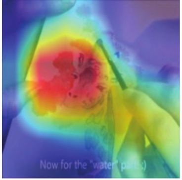
Table 4. Average out-of-distribution test accuracies on the DomainBed setting. Here we compare 14 domain generalization algorithms in
the exact same conditions. Note that we train domain validation set as a model selection method. † : Ours does not use IDCL and SWA
techniques due to implementational inflexibility on the DomainBed environment. Abbr. D: learning domain-invariant features by matching
distributions across different domains, A: Adversarial learning strategy, M : inter-domain mix-up, C: contrastive learning, U : unsupervised
domain adaptation, which is originally designed to take examples from the target domain during training.

Model             D A M C U CMNIST [1] RMNIST [16] VLCS [13] PACS [26] OfficeHome [42] TerraIncognita [2] DomainNet [34] Average

CORAL [38]        X           X   51.5 ± 0.1    98.0 ± 0.1   78.8 ± 0.6 86.2 ± 0.3   68.7 ± 0.3       47.6 ± 1.0       41.5 ± 0.1     67.5
              †
SelfReg (ours)    X     X X       52.1 ± 0.2    98.0 ± 0.1   77.8 ± 0.9 85.6 ± 0.4   67.9 ± 0.7       47.0 ± 0.3       42.8 ± 0.0     67.3

SagNet [32]       X X             51.7 ± 0.0    98.0 ± 0.0   77.8 ± 0.5 86.3 ± 0.2   68.1 ± 0.1       48.6 ± 1.0       40.3 ± 0.1     67.2
Mixup [45]              X         52.1 ± 0.2    98.0 ± 0.1   77.4 ± 0.6 84.6 ± 0.6   68.1 ± 0.3       47.9 ± 0.8       39.2 ± 0.1     66.7
MLDG [27]                         51.5 ± 0.1    97.9 ± 0.0   77.2 ± 0.4 84.9 ± 1.0   66.8 ± 0.6       47.7 ± 0.9       41.2 ± 0.1     66.7
ERM [41]                          51.5 ± 0.1    98.0 ± 0.0   77.5 ± 0.4 85.5 ± 0.2   66.5 ± 0.3       46.1 ± 1.8       40.9 ± 0.1     66.6
MTL [3]                           51.4 ± 0.1    97.9 ± 0.0   77.2 ± 0.4 84.6 ± 0.5   66.4 ± 0.5       45.6 ± 1.2       40.6 ± 0.1     66.2
RSC [22]                          51.7 ± 0.2    97.6 ± 0.1   77.1 ± 0.5 85.2 ± 0.9   65.5 ± 0.9       46.6 ± 1.0       38.9 ± 0.5     66.1
ARM [47]                          56.2 ± 0.2    98.2 ± 0.1   77.6 ± 0.3 85.1 ± 0.4   64.8 ± 0.3       45.5 ± 0.3       35.5 ± 0.2     66.1
DANN [15]         X X         X   51.5 ± 0.3    97.8 ± 0.1   78.6 ± 0.4 83.6 ± 0.4   65.9 ± 0.6       46.7 ± 0.5       38.3 ± 0.1     66.1
VREx [25]         X               51.8 ± 0.1    97.9 ± 0.1   78.3 ± 0.2 84.9 ± 0.6   66.4 ± 0.6       46.4 ± 0.6       33.6 ± 2.9     65.6
CDANN [29]        X X             51.7 ± 0.1    97.9 ± 0.1   77.5 ± 0.1 82.6 ± 0.9   65.8 ± 1.3       45.8 ± 1.6       38.3 ± 0.3     65.6
IRM [1]                           52.0 ± 0.1    97.7 ± 0.1   78.5 ± 0.5 83.5 ± 0.8   64.3 ± 2.2       47.6 ± 0.8       33.9 ± 2.8     65.4
GroupDRO [36] X                   52.1 ± 0.0    98.0 ± 0.0   76.7 ± 0.6 84.4 ± 0.8   66.0 ± 0.7       43.2 ± 1.1       33.3 ± 0.2     64.8
MMD [28]          X               51.5 ± 0.2    97.9 ± 0.0   77.5 ± 0.9 84.6 ± 0.5   66.3 ± 0.1       42.2 ± 1.6       23.4 ± 9.5     63.3

are designed to take examples from the target domain dur-                 [2] Sara Beery, Grant Van Horn, and Pietro Perona.
ing training – i.e. CORAL [38] is trained to minimize the                     Recognition in terra incognita. In Proceedings of the
distance between covariances of the source and target fea-                    European Conference on Computer Vision (ECCV),
tures. Note also that some studies [32, 15, 29] use the ad-                   pages 456–473, 2018. 7, 8, 14
versarial learning setting to obtain an unknown domain-
                                                                          [3] Gilles Blanchard, Aniket Anand Deshmukh, Urun Do-
invariant feature by fitting implicit generative models, such
                                                                              gan, Gyemin Lee, and Clayton Scott. Domain gener-
as GAN (generative adversarial networks). Though GAN is
                                                                              alization by marginal transfer learning. arXiv preprint
a powerful framework, the alternating gradient updates pro-
                                                                              arXiv:1711.07910, 2017. 7, 8, 13
cedure is often highly unstable and often results in mode
collapse [24].                                                            [4] Gilles Blanchard, Gyemin Lee, and Clayton Scott.
                                                                              Generalizing from several related classification tasks
6. Conclusion                                                                 to a new unlabeled sample. Advances in neural infor-
                                                                              mation processing systems, 24:2178–2186, 2011. 1
    In this paper, we proposed SelfReg, a new regulariza-
tion method for domain generalization that leverages a self-              [5] Fabio M Carlucci, Antonio D’Innocente, Silvia Bucci,
supervised contrastive regularization loss with only pos-                     Barbara Caputo, and Tatiana Tommasi. Domain gen-
itive data pairs, mitigating problems caused by negative                      eralization by solving jigsaw puzzles. In Proceedings
pair sampling. Our experiments on PACS dataset and Do-                        of the IEEE Conference on Computer Vision and Pat-
mainBed benchmarks show that our model matches or out-                        tern Recognition, pages 2229–2238, 2019. 2
performs prior work under the standard domain generaliza-                 [6] Junbum Cha, Hancheol Cho, Kyungjae Lee, Se-
tion evaluation setting. In future work, it would be interest-                unghyun Park, Yunsung Lee, and Sungrae Park. Do-
ing to extend SelfReg with the siamese network, enabling                      main generalization needs stochastic weight averaging
the model to choose better positive data pairs.                               for robustness on domain shifts, 2021. 4

References                                                                [7] Ting Chen, Simon Kornblith, Mohammad Norouzi,
                                                                              and Geoffrey Hinton. A simple framework for con-
 [1] Martin Arjovsky, Léon Bottou, Ishaan Gulrajani, and                     trastive learning of visual representations. In Interna-
     David Lopez-Paz. Invariant risk minimization. arXiv                      tional conference on machine learning, pages 1597–
     preprint arXiv:1907.02893, 2019. 7, 8, 12, 13                            1607. PMLR, 2020. 1, 2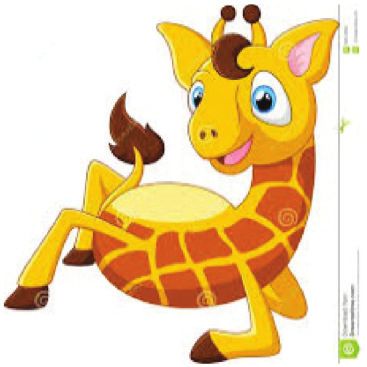
[8] Xinlei Chen and Kaiming He.         Exploring sim-         [19] Haowei He, Gao Huang, and Yang Yuan. Asymmetric
     ple siamese representation learning. arXiv preprint             valleys: Beyond sharp and flat local minima. arXiv
     arXiv:2011.10566, 2020. 2                                       preprint arXiv:1902.00744, 2019. 4
 [9] Jia Deng, Wei Dong, Richard Socher, Li-Jia Li, Kai         [20] Kaiming He, Haoqi Fan, Yuxin Wu, Saining Xie, and
     Li, and Li Fei-Fei. Imagenet: A large-scale hierarchi-          Ross Girshick. Momentum contrast for unsupervised
     cal image database. In 2009 IEEE conference on com-             visual representation learning. In Proceedings of the
     puter vision and pattern recognition, pages 248–255.            IEEE/CVF Conference on Computer Vision and Pat-
     Ieee, 2009. 5                                                   tern Recognition, pages 9729–9738, 2020. 1, 2
[10] Jeff Donahue, Yangqing Jia, Oriol Vinyals, Judy Hoff-      [21] Kaiming He, Xiangyu Zhang, Shaoqing Ren, and Jian
     man, Ning Zhang, Eric Tzeng, and Trevor Darrell. A              Sun. Deep residual learning for image recognition.
     deep convolutional activation feature for generic vi-           In Proceedings of the IEEE conference on computer
     sual recognition. UC Berkeley & ICSI, Berkeley, CA,             vision and pattern recognition, pages 770–778, 2016.
     USA. 1                                                          5
[11] Qi Dou, Daniel C Castro, Konstantinos Kamnitsas,           [22] Zeyi Huang, Haohan Wang, Eric P. Xing, and Dong
     and Ben Glocker. Domain generalization via model-               Huang. Self-challenging improves cross-domain gen-
     agnostic learning of semantic features. arXiv preprint          eralization. In ECCV, 2020. 4, 5, 6, 7, 8, 13
     arXiv:1910.13580, 2019. 2                                  [23] Pavel Izmailov, Dmitrii Podoprikhin, Timur Garipov,
[12] Antonio D’Innocente and Barbara Caputo. Domain                  Dmitry Vetrov, and Andrew Gordon Wilson. Averag-
     generalization with domain-specific aggregation mod-            ing weights leads to wider optima and better general-
     ules. In German Conference on Pattern Recognition,              ization. arXiv preprint arXiv:1803.05407, 2018. 4,
     pages 187–198. Springer, 2018. 2                                11, 13
[13] Chen Fang, Ye Xu, and Daniel N Rockmore. Unbiased          [24] Naveen Kodali, Jacob Abernethy, James Hays, and
     metric learning: On the utilization of multiple datasets        Zsolt Kira. On convergence and stability of gans.
     and web images for softening bias. In Proceedings of            arXiv preprint arXiv:1705.07215, 2017. 8
     the IEEE International Conference on Computer Vi-          [25] David Krueger, Ethan Caballero, Joern-Henrik Jacob-
     sion, pages 1657–1664, 2013. 7, 8, 12                           sen, Amy Zhang, Jonathan Binas, Dinghuai Zhang,
[14] Chelsea Finn, Pieter Abbeel, and Sergey Levine.                 Remi Le Priol, and Aaron Courville.              Out-of-
     Model-agnostic meta-learning for fast adaptation of             distribution generalization via risk extrapolation (rex).
     deep networks. In International Conference on Ma-               arXiv preprint arXiv:2003.00688, 2020. 7, 8, 13
     chine Learning, pages 1126–1135. PMLR, 2017. 2             [26] Da Li, Yongxin Yang, Yi-Zhe Song, and Timothy
[15] Yaroslav Ganin, Evgeniya Ustinova, Hana Ajakan,                 Hospedales. Deeper, broader and artier domain gen-
     Pascal Germain, Hugo Larochelle, François Lavi-                eralization. In International Conference on Computer
     olette, Mario Marchand, and Victor Lempitsky.                   Vision, 2017. 2, 5, 6, 7, 8, 13
     Domain-adversarial training of neural networks. The        [27] Da Li, Yongxin Yang, Yi-Zhe Song, and Timothy
     journal of machine learning research, 17(1):2096–               Hospedales. Learning to generalize: Meta-learning for
     2030, 2016. 1, 2, 7, 8, 13                                      domain generalization. In Proceedings of the AAAI
[16] Muhammad Ghifary, W Bastiaan Kleijn, Mengjie                    Conference on Artificial Intelligence, volume 32,
     Zhang, and David Balduzzi. Domain generalization                2018. 2, 7, 8, 13
     for object recognition with multi-task autoencoders.       [28] Haoliang Li, Sinno Jialin Pan, Shiqi Wang, and Alex C
     In Proceedings of the IEEE international conference             Kot. Domain generalization with adversarial feature
     on computer vision, pages 2551–2559, 2015. 7, 8, 12             learning. In Proceedings of the IEEE Conference
[17] Jean-Bastien Grill, Florian Strub, Florent Altché,             on Computer Vision and Pattern Recognition, pages
     Corentin Tallec, Pierre H Richemond, Elena                      5400–5409, 2018. 1, 2, 5, 7, 8, 13
     Buchatskaya, Carl Doersch, Bernardo Avila Pires,           [29] Ya Li, Xinmei Tian, Mingming Gong, Yajing Liu,
     Zhaohan Daniel Guo, Mohammad Gheshlaghi                         Tongliang Liu, Kun Zhang, and Dacheng Tao. Deep
     Azar, et al. Bootstrap your own latent: A new                   domain generalization via conditional invariant adver-
     approach to self-supervised learning. arXiv preprint            sarial networks. In Proceedings of the European Con-
     arXiv:2006.07733, 2020. 2, 3                                    ference on Computer Vision (ECCV), pages 624–639,
[18] Ishaan Gulrajani and David Lopez-Paz. In search                 2018. 1, 2, 7, 8, 13
     of lost domain generalization.        arXiv preprint       [30] Saeid Motiian, Marco Piccirilli, Donald A Adjeroh,
     arXiv:2007.01434, 2020. 2, 7, 12, 13, 14                        and Gianfranco Doretto. Unified deep supervised do-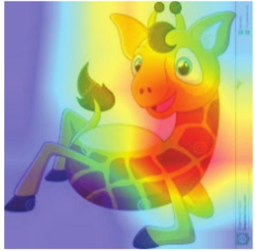
main adaptation and generalization. In Proceedings of         hashing network for unsupervised domain adaptation.
     the IEEE international conference on computer vision,         In Proceedings of the IEEE conference on computer
     pages 5715–5725, 2017. 2                                      vision and pattern recognition, pages 5018–5027,
[31] Krikamol Muandet, David Balduzzi, and Bernhard                2017. 7, 8, 14
     Schölkopf. Domain generalization via invariant fea-     [43] Yufei Wang, Haoliang Li, and Alex C Kot. Hetero-
     ture representation. In International Conference on           geneous domain generalization via domain mixup. In
     Machine Learning, pages 10–18. PMLR, 2013. 1, 2               ICASSP 2020-2020 IEEE International Conference on
[32] Hyeonseob Nam, HyunJae Lee, Jongchan Park, Won-               Acoustics, Speech and Signal Processing (ICASSP),
     jun Yoon, and Donggeun Yoo. Reducing domain                   pages 3622–3626. IEEE, 2020. 2, 4
     gap via style-agnostic networks.    arXiv preprint       [44] Minghao Xu, Jian Zhang, Bingbing Ni, Teng Li,
     arXiv:1910.11645, 2019. 2, 7, 8, 13                           Chengjie Wang, Qi Tian, and Wenjun Zhang. Ad-
[33] Aaron van den Oord, Yazhe Li, and Oriol Vinyals.              versarial domain adaptation with domain mixup. In
     Representation learning with contrastive predictive           Proceedings of the AAAI Conference on Artificial In-
     coding. arXiv preprint arXiv:1807.03748, 2018. 1,             telligence, volume 34, pages 6502–6509, 2020. 2
     2                                                        [45] Shen Yan, Huan Song, Nanxiang Li, Lincan Zou,
                                                                   and Liu Ren.       Improve unsupervised domain
[34] Xingchao Peng, Qinxun Bai, Xide Xia, Zijun Huang,
                                                                   adaptation with mixup training.     arXiv preprint
     Kate Saenko, and Bo Wang. Moment matching for
                                                                   arXiv:2001.00677, 2020. 2, 7, 8, 13
     multi-source domain adaptation. In Proceedings of the
     IEEE International Conference on Computer Vision,        [46] Hongyi Zhang, Moustapha Cisse, Yann N Dauphin,
     pages 1406–1415, 2019. 7, 8, 14                               and David Lopez-Paz. mixup: Beyond empirical
                                                                   risk minimization. arXiv preprint arXiv:1710.09412,
[35] Xingchao Peng, Baochen Sun, Karim Ali, and Kate
                                                                   2017. 4
     Saenko. Learning deep object detectors from 3d mod-
     els. In Proceedings of the IEEE International Con-       [47] Marvin Zhang, Henrik Marklund, Abhishek Gupta,
     ference on Computer Vision, pages 1278–1286, 2015.            Sergey Levine, and Chelsea Finn. Adaptive risk
     1                                                             minimization: A meta-learning approach for tackling
                                                                   group shift. arXiv preprint arXiv:2007.02931, 2020.
[36] Shiori Sagawa, Pang Wei Koh, Tatsunori B
                                                                   7, 8, 13
     Hashimoto, and Percy Liang.           Distributionally
     robust neural networks for group shifts: On the impor-   [48] Han Zhao, Remi Tachet Des Combes, Kun Zhang, and
     tance of regularization for worst-case generalization.        Geoffrey Gordon. On learning invariant representa-
     arXiv preprint arXiv:1911.08731, 2019. 7, 8, 13               tions for domain adaptation. In International Confer-
                                                                   ence on Machine Learning, pages 7523–7532. PMLR,
[37] Ramprasaath R Selvaraju, Michael Cogswell, Ab-                2019. 4
     hishek Das, Ramakrishna Vedantam, Devi Parikh, and
     Dhruv Batra. Grad-cam: Visual explanations from
     deep networks via gradient-based localization. In
     Proceedings of the IEEE international conference on
     computer vision, pages 618–626, 2017. 6
[38] Baochen Sun and Kate Saenko. Deep coral: Correla-
     tion alignment for deep domain adaptation. In Euro-
     pean conference on computer vision, pages 443–450.
     Springer, 2016. 1, 2, 7, 8, 13
[39] Laurens Van der Maaten and Geoffrey Hinton. Visu-
     alizing data using t-sne. Journal of machine learning
     research, 9(11), 2008. 5
[40] V Vapnik. Statistical learning theory new york. NY:
     Wiley, 1998. 1, 2
[41] Vladimir N Vapnik. An overview of statistical learn-
     ing theory. IEEE transactions on neural networks,
     10(5):988–999, 1999. 7, 8, 12, 13, 14
[42] Hemanth Venkateswara, Jose Eusebio, Shayok
     Chakraborty, and Sethuraman Panchanathan. Deep
Appendix
In Table 5-11, SelfReg (ours)† does not include Inter-
domain Curriculum Learning (IDCL) and SelfReg with
stochastic weight averaging (SWA) [23] techniques. How-
ever, note that Table 8 provides the performance of our Sel-
fReg with SWA technique also. Since DomainBed is sup-
posed to be evaluated every N steps, we needed to modify
the code to apply the SWA technique. We modified the code
to evaluate model on the test set after completing 5000 steps
learning with SWA techniques. We used ”–single test envs”
option because the required amount of computation for the
cross-validation model selection method was too much for
us.Table 5. Detailed scores on ColoredMNIST [1] in DomainBed [18].
Model selection: training-domain validation set
Algorithm +90% +80% -90% Avg
†
SelfReg (ours) 72.2 ± 0.5 73.7 ± 0.2 10.5 ± 0.3 52.1 ± 0.2
ERM [41] 71.7 ± 0.1 72.9 ± 0.2 10.0 ± 0.1 51.5
Model selection: test-domain validation set (oracle)
Algorithm +90% +80% -90% Avg
SelfReg (ours)† 71.3 ± 0.4 73.4 ± 0.2 29.3 ± 2.1 58.0 ± 0.7
ERM [41] 71.8 ± 0.4 72.9 ± 0.1 28.7 ± 0.5 57.8
Table 6. Detailed scores on RotatedMNIST [16] in DomainBed [18].
Model selection: training-domain validation set
Algorithm 0 15 30 45 60 75 Avg
†
SelfReg (ours) 95.7 ± 0.3 99.0 ± 0.1 98.9 ± 0.1 99.0 ± 0.1 98.9 ± 0.1 96.6 ± 0.1 98.0 ± 0.2
ERM [41] 95.9 ± 0.1 98.9 ± 0.0 98.8 ± 0.0 98.9 ± 0.0 98.9 ± 0.0 96.4 ± 0.0 98.0
Model selection: test-domain validation set (oracle)
Algorithm 0 15 30 45 60 75 Avg
†
SelfReg (ours) 96.0 ± 0.3 98.9 ± 0.1 98.9 ± 0.1 98.9 ± 0.1 98.9 ± 0.1 96.8 ± 0.1 98.1 ± 0.7
ERM [41] 95.3 ± 0.2 98.7 ± 0.1 98.9 ± 0.1 98.7 ± 0.2 98.9 ± 0.0 96.2 ± 0.2 97.8
Table 7. Detailed scores on VLCS [13] in DomainBed [18].
Model selection: training-domain validation set
Algorithm C L S V Avg
†
SelfReg (ours) 96.7 ± 0.4 65.2 ± 1.2 73.1 ± 1.3 76.2 ± 0.7 77.8 ± 0.9
ERM [41] 97.7 ± 0.4 64.3 ± 0.9 73.4 ± 0.5 74.6 ± 1.3 77.5
Model selection: test-domain validation set (oracle)
Algorithm C L S V Avg
†
SelfReg (ours) 97.9 ± 0.4 66.7 ± 0.1 73.5 ± 0.7 74.7 ± 0.7 78.2 ± 0.1
ERM [41] 97.6 ± 0.3 67.9 ± 0.7 70.9 ± 0.2 74.0 ± 0.6 77.6Table 8. Detailed scores on PACS [26] in DomainBed [18]. Note that we provide the performance of our SelfReg applied with SWA [23]
technique also.
Model selection: training-domain validation set
Algorithm A C P S Avg
SelfReg with SWA (ours) 85.9 ± 0.6 81.9 ± 0.4 96.8 ± 0.1 81.4 ± 0.6 86.5 ± 0.3
SagNet [32] 87.4 ± 1.0 80.7 ± 0.6 97.1 ± 0.1 80.0 ± 0.4 86.3
CORAL [38] 88.3 ± 0.2 80.0 ± 0.5 97.5 ± 0.3 78.8 ± 1.3 86.2
SelfReg (ours)† 87.9 ± 1.0 79.4 ± 1.4 96.8 ± 0.7 78.3 ± 1.2 85.6 ± 0.4
ERM [41] 84.7 ± 0.4 80.8 ± 0.6 97.2 ± 0.3 79.3 ± 1.0 85.5
RSC [22] 85.4 ± 0.8 79.7 ± 1.8 97.6 ± 0.3 78.2 ± 1.2 85.2
ARM [47] 86.8 ± 0.6 76.8 ± 0.5 97.4 ± 0.3 79.3 ± 1.2 85.1
VREx [25] 86.0 ± 1.6 79.1 ± 0.6 96.9 ± 0.5 77.7 ± 1.7 84.9
MLDG [27] 85.5 ± 1.4 80.1 ± 1.7 97.4 ± 0.3 76.6 ± 1.1 84.9
MMD [28] 86.1 ± 1.4 79.4 ± 0.9 96.6 ± 0.2 76.5 ± 0.5 84.6
Mixup [45] 86.1 ± 0.5 78.9 ± 0.8 97.6 ± 0.1 75.8 ± 1.8 84.6
MTL [3] 87.5 ± 0.8 77.1 ± 0.5 96.4 ± 0.8 77.3 ± 1.8 84.6
GroupDRO [36] 83.5 ± 0.9 79.1 ± 0.6 96.7 ± 0.3 78.3 ± 2.0 84.4
DANN [15] 86.4 ± 0.8 77.4 ± 0.8 97.3 ± 0.4 73.5 ± 2.3 83.6
IRM [1] 84.8 ± 1.3 76.4 ± 1.1 96.7 ± 0.6 76.1 ± 1.0 83.5
CDANN [29] 84.6 ± 1.8 75.5 ± 0.9 96.8 ± 0.3 73.5 ± 0.6 82.6
Model selection: test-domain validation set (oracle)
Algorithm A C P S Avg
SelfReg with SWA (ours) 87.5 ± 0.1 83.0 ± 0.1 97.6 ± 0.1 82.8 ± 0.2 87.7 ± 0.1
SagNet [32] 87.4 ± 0.5 81.2 ± 1.2 96.3 ± 0.8 80.7 ± 1.1 86.4
CORAL [38] 86.6 ± 0.8 81.8 ± 0.9 97.1 ± 0.5 82.7 ± 0.6 87.1
SelfReg (ours)† 87.9 ± 0.5 80.6 ± 1.1 97.1 ± 0.4 81.1 ± 1.3 86.7 ± 0.8
ERM [41] 86.5 ± 1.0 81.3 ± 0.6 96.2 ± 0.3 82.7 ± 1.1 86.7
RSC [22] 86.0 ± 0.7 81.8 ± 0.9 96.8 ± 0.7 80.4 ± 0.5 86.2
ARM [47] 85.0 ± 1.2 81.4 ± 0.2 95.9 ± 0.3 80.9 ± 0.5 85.8
VREx [25] 87.8 ± 1.2 81.8 ± 0.7 97.4 ± 0.2 82.1 ± 0.7 87.2
MLDG [27] 87.0 ± 1.2 82.5 ± 0.9 96.7 ± 0.3 81.2 ± 0.6 86.8
MMD [28] 88.1 ± 0.8 82.6 ± 0.7 97.1 ± 0.5 81.2 ± 1.2 87.2
Mixup [45] 87.5 ± 0.4 81.6 ± 0.7 97.4 ± 0.2 80.8 ± 0.9 86.8
MTL [3] 87.0 ± 0.2 82.7 ± 0.8 96.5 ± 0.7 80.5 ± 0.8 86.7
GroupDRO [36] 87.5 ± 0.5 82.9 ± 0.6 97.1 ± 0.3 81.1 ± 1.2 87.1
DANN [15] 87.0 ± 0.4 80.3 ± 0.6 96.8 ± 0.3 76.9 ± 1.1 85.2
IRM [1] 84.2 ± 0.9 79.7 ± 1.5 95.9 ± 0.4 78.3 ± 2.1 84.5
CDANN [29] 87.7 ± 0.6 80.7 ± 1.2 97.3 ± 0.4 77.6 ± 1.5 85.8Table 9. Detailed scores on OfficeHome [42] in DomainBed [18].
Model selection: training-domain validation set
Algorithm A C P R Avg
†
SelfReg (ours) 63.6 ± 1.4 53.1 ± 1.0 76.9 ± 0.4 78.1 ± 0.4 67.9 ± 0.7
ERM [41] 61.3 ± 0.7 52.4 ± 0.3 75.8 ± 0.1 76.6 ± 0.3 66.5
Model selection: test-domain validation set (oracle)
Algorithm A C P R Avg
†
SelfReg (ours) 64.2 ± 0.6 53.6 ± 0.7 76.7 ± 0.3 77.9 ± 0.5 68.1 ± 0.3
ERM [41] 61.7 ± 0.7 53.4 ± 0.3 74.1 ± 0.4 76.2 ± 0.6 66.4
Table 10. Detailed scores on TerraIncognita [2] in DomainBed [18].
Model selection: training-domain validation set
Algorithm L100 L38 L43 L46 Avg
†
SelfReg (ours) 48.8 ± 0.9 41.3 ± 1.8 57.3 ± 0.7 40.6 ± 0.9 47.0 ± 0.3
ERM [41] 49.8 ± 4.4 42.1 ± 1.4 56.9 ± 1.8 35.7 ± 3.9 46.1
Model selection: test-domain validation set (oracle)
Algorithm L100 L38 L43 L46 Avg
†
SelfReg (ours) 60.0 ± 2.3 48.8 ± 1.0 58.6 ± 0.8 44.0 ± 0.6 52.8 ± 0.9
ERM [41] 59.4 ± 0.9 49.3 ± 0.6 60.1 ± 1.1 43.2 ± 0.5 53.0
Table 11. Detailed scores on DomainNet [34] in DomainBed [18]. Note that SelfReg† achived the-state-of-the-art.
Model selection: training-domain validation set
Algorithm Clip Info Paint Quick Real Sketch Avg
†
SelfReg (ours) 60.7 ± 0.1 21.6 ± 0.1 49.4 ± 0.2 12.7 ± 0.1 60.7 ± 0.1 51.7 ± 0.1 42.8 ± 0.0
ERM [41] 58.1 ± 0.3 18.8 ± 0.3 46.7 ± 0.3 12.2 ± 0.4 59.6 ± 0.1 49.8 ± 0.4 40.9
Model selection: test-domain validation set (oracle)
Algorithm Clip Info Paint Quick Real Sketch Avg
SelfReg (ours)† 60.7 ± 0.1 21.6 ± 0.1 49.5 ± 0.1 14.2 ± 0.3 60.7 ± 0.1 51.7 ± 0.1 43.1 ± 0.1
ERM [41] 58.6 ± 0.3 19.2 ± 0.2 47.0 ± 0.3 13.2 ± 0.2 59.9 ± 0.3 49.8 ± 0.4 41.3You can also read