Impact of Ensemble-Variational Data Assimilation in Heavy Rain Forecast over Brazilian Northeast
←
→
Page content transcription
If your browser does not render page correctly, please read the page content below
atmosphere

Article
Impact of Ensemble-Variational Data Assimilation in Heavy
Rain Forecast over Brazilian Northeast
João Pedro Gonçalves Nobre *,† , Éder Paulo Vendrasco † and Carlos Frederico Bastarz †

                                          National Institute for Space Research (INPE), Cachoeira Paulista 12630-970, Brazil;
                                          eder.vendrasco@inpe.br (É.P.V.); carlos.bastarz@inpe.br (C.F.B.)
                                          * Correspondence: joao.nobre@inpe.br
                                          † These authors contributed equally to this work.

                                          Abstract: The Brazilian Northeast (BNE) is located in the tropical region of Brazil. It is bounded
                                          by the Atlantic Ocean, and its climate and vegetation are strongly affected by continental plateaus.
                                          The plateaus keep the humid air masses to the east and are responsible for the rain episodes,
                                          and at the west side the northeastern hinterland and dry air masses are observed. This work is
                                          a case study that aims to evaluate the impact of updating the model initial condition using the
                                          3DEnVar (Three-Dimensional Ensemble Variational) system in heavy rain episodes associated with
                                          Mesoscale Convective Systems (MCS). The results were compared to 3DVar (Three-Dimensional
                                          Variational) and EnSRF (Ensemble Square Root Filter) systems and with no data assimilation. The
                                          study enclosed two MCS cases occurring on 14 and 24 January 2017. For that purpose, the RMS
                                          (Regional Modeling System) version 3.0.0, maintained by the Center for Weather Forecasting and
                                Climate Studies (CPTEC), used two components: the Weather Research and Forecasting (WRF)
                                   mesoscale model and the GSI (Gridpoint Statistical Interpolation) data assimilation system. Currently,
Citation: Gonçalves Nobre, J.P.;          the RMS provides the WRF initial conditions by using 3DVar data assimilation methodology. The
Vendrasco, E.P.; Bastarz, C.F. Impact     3DVar uses a climatological covariance matrix to minimize model errors. In this work, the 3DEnVar
of Ensemble-Variational Data              updates the RMS climatological covariance matrix through the forecast members based on the
Assimilation in Heavy Rain Forecast       errors of the day. This work evaluated the improvements in the detection and estimation of 24 h
over Brazilian Northeast. Atmosphere      accumulated precipitation in MCS events. The statistic index RMSE (Root Mean Square Error)
2021, 12, 1201. https://doi.org/
                                          showed that the hybrid data assimilation system (3DEnVar) performed better in reproducing the
10.3390/atmos12091201
                                          precipitation in the MCS occurred on 14 January 2017. On 24 January 2017, the EnSRF was the best
                                          system for improving the WRF forecast. In general, the BIAS showed that the WRF initialized with
Academic Editors: Avelino F.
                                          different initial conditions overestimated the 24 h accumulated precipitation. Therefore, the viability
Arellano and Yunheng Wang
                                          of using a hybrid system may depend on the hybrid algorithm that can modify the weights attributed
Received: 12 July 2021                    to the EnSRF and 3DVar matrix in the GSI over the assimilation cycles.
Accepted: 24 August 2021
Published: 16 September 2021              Keywords: 3DEnVar; mesoscale convective systems; WRF; GSI

Publisher’s Note: MDPI stays neutral
with regard to jurisdictional claims in
published maps and institutional affil-   1. Introduction
iations.                                       Accurate weather forecasts of severe weather phenomena that affects the economy
                                          across the globe are essential for short to long-term planning of various human activities
                                          in order to avoid socio-economic damage caused by natural disasters (e.g., landslides
                                          and floods). For the Brazilian Northeast (BNE), which is the region of study of this work,
Copyright: © 2021 by the authors.         according to data from the portal of the National Confederation of Cities [1] for a long
Licensee MDPI, Basel, Switzerland.        dry period, BNE had losses totaled in the order of BRL 52 billion between 2012 and 2015.
This article is an open access article    For the same region, intense rain events have caused deaths, floods, and rupture of dams,
distributed under the terms and           causing many social and economic losses in only one day [2].
conditions of the Creative Commons             It is essential to have a good representation of the initial conditions of the atmosphere
Attribution (CC BY) license (https://     in order to obtain an accurate weather forecast. The initialization of Numerical Weather
creativecommons.org/licenses/by/
                                          Predictions (NWP) means calculating many dynamic and thermodynamic parameters. An
4.0/).

Atmosphere 2021, 12, 1201. https://doi.org/10.3390/atmos12091201                                           https://www.mdpi.com/journal/atmosphere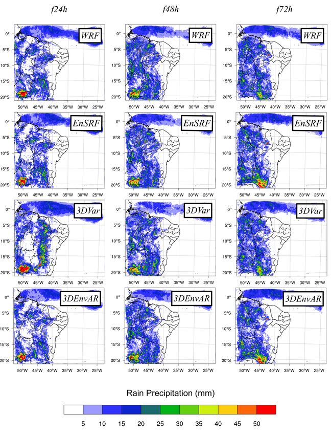
Atmosphere 2021, 12, 1201                                                                                            2 of 20

                            alternative method for improving the initial conditions for an NWP model is by using Data
                            Assimilation (DA). DA systems organize the information in the model’s grid using the
                            best estimation of the initial state. Thus, DA techniques must combine observations (e.g.,
                            meteorological, oceanographic, or hydrological) with a background. The result is the best
                            initial condition for the NWP models initialization [3].
                                  Initially, a subjective DA method used the same wind velocity values (isopleths) to
                            interpolate the observation fields. The scheme was known as Subjective Interpolation [4].
                            This scheme demanded an experienced synoptic meteorologist and many days of work
                            (e.g., data preparation and remotion of observational errors), which resulted in hard work
                            for operational application.
                                  An important fact to consider is that meteorological observations are not perfect
                            because of intrinsic observation errors and human interference (e.g., parallax errors). In
                            order to avoid observation errors, a climatology, the mean of neighbor stations, and a
                            weather forecast may be the reference in the DA algorithm schemes [5]. If large differences
                            between observed and background data exist, the observation should not be considered in
                            the DA procedure.
                                  Many objective analysis schemes were developed during the last century. These
                            schemes replaced subjective interpolation by avoiding manual errors caused by erroneous
                            meteorologist’s interpretations. From that perspective, References [4,6] introduced a poly-
                            nomial interpolation method, and [7] developed a Successive Correction Method (SCM).
                            A similar SCM method, introduced by [8] gained notoriety. This method combines me-
                            teorological observational data with the model background in order to improve initial
                            conditions. Afterwards, a statistical correction method acquired notoriety when it was
                            compared with SCM, and it was presented to the scientific community by [9,10]. Finally,
                            the Variational Method (VM) was introduced by [11], and a spectral operational DA system
                            by [12].
                                  In general, DA divides into sequential and non-sequential techniques [13]. Sequential
                            methods (e.g., 3DVar and EnSRF) consist of the DA methods where many analysis cycles are
                            applied at each time step in order to obtain a new model initial condition. Non-sequential
                            methods (e.g., 4DVar) corrects the model trajectory when the observations are available in
                            a typical forecast time window of 6 h.
                                  The Center for Weather Forecasting and Climate Studies at the National Institute for
                            Space Research (CPTEC/INPE in Portuguese) developed the Regional Modelling System
                            (RMS), which allow coupling different weather forecast models such as WRF and DA
                            systems such as GSI (Gridpoint Statistical Interpolation) and WRFDA (WRF DA system).
                            RMS permits updating the initial condition from the CPTEC’s operational WRF model
                            with conventional and non-conventional datasets using the GSI system, and it allows
                            performing 3DVar, EnSRF, and 3DEnVar DA.
                                  Encouraging results have been obtained in several studies using 3DEnVar DA. Refer-
                            ence [14] observed that the hybrid using the radar radial speed produces better analysis
                            and prediction compared to the result without DA during Hurricane Ika (2008). Refer-
                            ence [15] used hybrid DA with radar data to improve the analysis and predictions of a
                            storm event on 20 May 1977, near Dell City in Oklahoma and obtained satisfactory results.
                            Reference [16] carried out a detailed study using the CPTEC global model in order to assess
                            the ability of the hybrid system to assimilate data from conventional stations, satellites, and
                            predict certain variables. The conclusion was that the 3DEnVar had better results compared
                            to 3DVar in all cases. The benefits obtained by using the 3DEnVar were due to the errors of
                            the day incorporated into the background covariance matrix.
                                  Therefore, the main objective of this work is to incorporate daily forecast errors to
                            update analyses by EnSRF using the 3DEnVar and to evaluate how the hybrid DA system
                            (3dEnVar) can improve the daily precipitation forecast by the WRF model during Mesoscale
                            Convective Systems (MCS) events occurred over the Brazilian Northeast (BNE).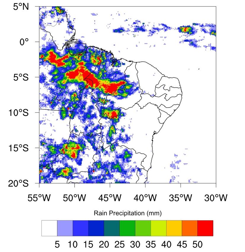
Atmosphere 2021, 12, 1201                                                                                            3 of 20

                            2. Materials and Methods
                                 The MCS events studied in this work occurred on 14th and 24th January 2017. These
                            two cases were selected because they were the two most heavy-rain events in 2017 over
                            Maranhao state. Both cases were associated with Mesoscale Convective Systems (MCS) and
                            generated 24 h accumulated precipitation over 70 mm. According to [17], the BNE has high
                            occurrence of MCS.This work presents an impact evaluation of the 3DVar and 3DEnVar DA
                            systems in improving precipitation forecasts from the WRF model for a domain over the
                            BNE. Thereby, Section 2 illustrates the 3DVar and 3DEnVar main characteristics, the WRF
                            configurations, and a description of the statistic metrics used to evaluate the DA analyses
                            and WRF forecasts.

                            2.1. Location of the Study Area
                                 BNE (Figure 1) is located in the tropical portion of Brazil between the equator (0◦ S) and
                            Capricorn parallels (23.5◦ S). The mean surface temperature of this region is around 20 degrees
                            Celsius, and it has a heterogeneous topography (at the coast it has plains bounded by the
                            Atlantic Ocean, and at the hinterland it has highlands responsible for the dry meteorological
                            conditions).

                            Figure 1. Brazilian Northeast topographic domain (m).

                                 The domain showed in Figure 1 was also used to assess the rainfall events associated
                            with MCS over the BNE using the WRF model and satellite rainfall estimates. The domain
                            area chosen in this study considered the dynamic and geographic particularities of the
                            synoptic systems (e.g., upper-level cyclonic vortex, Intertropical Convergence Zone, and
                            sea breeze) that produce MCS in BNE.

                            2.2. Convective Systems Identification
                                 MCS is a cloud system with an area of equal to or more than 3500 km2 , and the cloud
                            top brightness temperature is equal to or less than −38.5 degrees Celsius [18]. The infrared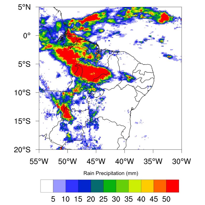
Atmosphere 2021, 12, 1201                                                                                           4 of 20

                            channel images from the GOES-13 (Geostationary Operational Environmental Satellite-
                            13) sensor provided the cloud top brightness temperature, and they are available at the
                            Division of Meteorological Satellites and Sensors website (http://satelite.cptec.inpe.br/,
                            (accessed on 25 August 2021)).

                            2.3. Rain Events Identification
                                 The 24 h accumulated precipitation observations were obtained from the National
                            Meteorological Institute (INMET). It was useful for identifying heavy rain precipitation
                            episodes that occurred over BNE meteorological stations. The heavy rain precipitation, in
                            this work, is an event in which the 24 h accumulated precipitation registered by the BNE
                            meteorological stations was greater than 70 mm occurring on 14 and 24 January 2017. This
                            reference value is the same one adopted by the National Center for Monitoring and Early
                            Warning of Natural Disasters (CEMADEN), available on https://www.gov.br/mcti/pt-br/
                            rede-mcti/cemaden, (accessed on 25 August 2021).
                                 In order to spatially evaluate the WRF heavy rain forecasts over the BNE, the MERGE
                            data [19] were chosen. The MERGE is an operational product produced and distributed by
                            CPTEC. It combines the observed precipitation with the estimate of precipitation by satellite.
                            Therefore, the MERGE algorithm combines the Integrated Multi-satellite Retrievals for
                            GPM (IMERG) and TRMM Multisatellite Precipitation Analysis (TRMM-TMPA) with
                            observations, and the final data are available with 0.1 degrees horizontal resolution.

                            2.4. WRF Mesoscale Model
                                 WRF is a NWP model developed by the National Center for Atmospheric Research
                            (NCAR), from the University Corporation for Atmospheric Research (UCAR). It is the most
                            widely used dynamical downscaling numerical weather forecasting and research model.
                            The WRF model is also continuously improved and supported by a wide international
                            atmospheric science research community [20].
                                 This work used Advanced Research WRF 3.9.1.1, the same operational version used by
                            CPTEC. The WRF consists of two dynamic cores, a DA system and a software architecture
                            structure, which supports parallel computing applied to solve a series of meteorological
                            problems ranging from the meter scale to thousands of kilometers [21].
                                 The WRF model used the same parameterizations defined by [22], except for the
                            Cumulus cloud parameterizations. This modification occurred because the climatological
                            study [23] for the tropical region between 2012 and 2016 summer showed that the new
                            Tiedke schemes combined with RRTMG were the best schemes for reproducing diurnal
                            precipitation cycle between 45 degrees north–south. The authors in [23] compared the
                            new Tiedke [24], the Tiedke [25], the Kain–Fritsch [26], and the new simplified Arakawa–
                            Schubert schemes [27]. Moreover, the parameterizations used in our study (Table 1) are the
                            same ones employed by CPTEC in its operational WRF model.

                            Table 1. The WRF model configurations.

                                            Parameters                                  Configurations
                                              Model                                          WRF
                                      Horizontal Resolution                                  9 km
                                          Global Model                                     GEFS [28]
                                        Topographic data                               SRTM (30 m) [29]
                                            Soil data                                   MODIS (925 m)
                                        Radiation model                                   RRTMG [30]
                                          Vertical levels                              42 sigma-pressure
                                          Microphysics                                     WSM6 [31]
                                            Cumulus                                    New Tiedtke [24]
                                       Planetary boundary                                   YSU [32]
                                          Surface model                                    Noah [33]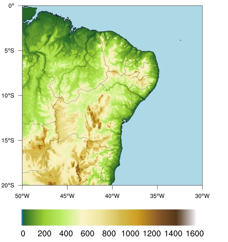
Atmosphere 2021, 12, 1201                                                                                          5 of 20

                                 The GEFS [28] is an ensemble NWP model from the National Centers for Environmen-
                            tal Prediction (NCEP), consisting of 21 members with a horizontal and vertical resolution
                            of 1 degree and 64 vertical levels. Although GEFS forecasts are currently available four
                            times a day on a 0.5 degrees latitude-longitude grid, we used the 0000 UTC initialized runs
                            on a 1.0 degree latitude-longitude grid since this is the only initialization time and output
                            grid spacing available on the NCEP NOMADS server for the MCS forecast periods.
                                 The WRF initial conditions were from GEFS, and GEFS was updated by 3DVar, EnSRF,
                            and 3DEnVar DA systems. The 3DVar system updated only the GEFS control member, and
                            the EnSRF and 3DEnVar updated the 21 forecast members from GEFS (20 perturbations
                            + 1 control member). For later times in the 6 h cycle, the WRF 6 h forecasts were updated
                            by 3DVar, EnSRF, and 3DEnVar. Therefore, a 6 h cycle from 12 and 22 to 14 (MCS 1) and
                            24 January (MCS 2) 0000 UTC was performed, and 72/48/24 h forecasts were initiated at
                            12/13/14 January 0000 UTC (MCS 1) and 22/23/240000 UTC (MCS 2). The precipitation
                            forecasts identified by f72, f48, and f24 stands for the 24 h accumulated precipitation
                            forecasts valid for 14 January (MCS 1) and 24 (MCS 2) and initiated at each 0000 UTC cycle
                            as mentioned above.

                            2.5. The Gridpoint Statistical Interpolation
                                 The Regional Modelling System from CPTEC used in this work applied the Gridpoint
                            Statistical Interpolation (GSI) DA scheme to update the analyses. Thus, in order to update
                            the forecasts, GEFS (in the first assimilation cycle) and WRF data (in the other assimilation
                            cycles) were combined with meteorological observations using 3DEnVar DA systems.

                            2.5.1. Data Assimilated
                                 At the analysis step in the assimilation cycle, the GSI used the radiance data from
                            the Advanced Microwave Sounding Unit-A (AMSU-A); the data from the Meteorological
                            Operational Satellite Program (METOP)-A/B and Microwave Humidity Sounder (MHS)
                            containing microwave moisture sounding information from NOAA-18, 19, and METOP-
                            A/B satellites data; the High-Resolution Infrared Radiation Sounder 4 (HIRS4) data, with
                            radiance from NOAA-18, 19, and METOP-A/B satellites; observational wind data by
                            satellite, curvature angle data, and GPS radio-concealment, plus data from conventional
                            and automatic weather stations on the surface; and radiosonde, for zonal and southern
                            winds, temperature, specific humidity, and surface pressure, available at the following
                            website: https://rda.ucar.edu, (accessed on 25 August 2021).

                            2.5.2. 3DVar Variational Method
                                 The 3DVar uses an iterative method to generate atmospheric analyses based on an
                            algorithm that requires an efficient solution search process (e.g., the conjugate gradient
                            minimization algorithm).
                                 The main objective of the variational problem is to find a minimum variance analysis
                            that minimizes the cost function (Equation (1)). In order to perform this, it is necessary
                            to calculate the difference between the state estimate x and the background xb weighted
                            by the inverse error of the background error covarianvce B in addition to the difference
                            between the observation vector yo and the background state at the physical space H(x),
                            weighted by the inverse of the observation error covariance matrix R.

                                                   1                           1
                                         J (x) =     (x − xb )T B−1 (x − xb ) + [yo − H (x)]T (R)−1 [yo − H (x)]      (1)
                                                   2                           2
                                 In Equation (1), the vector x − xb represents the analysis increment (errors). In the
                            same expression, y − H (x) is the innovation, with H being the non-linear observation
                            operator responsible for bringing the state vector to be analyzed to the physical space of
                            the observation.
                                 The NMC method [34] was used in this work to generate the climatological back-
                            ground error statistics (B). A dataset containing 3 months of cold-start 24 h forecasts over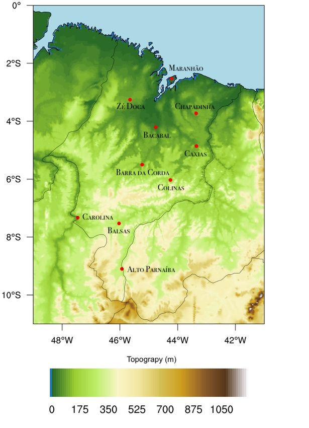
Atmosphere 2021, 12, 1201                                                                                          6 of 20

                            the entire South America covering the Southern Hemisphere during the summer was
                            produced every day starting at 0000 and 1200 UTC. The differences between the 24 and 12 h
                            forecasts valid at the same time were used to calculate the domain-averaged background
                            error statistics.
                                  In order to obtain the analysis equation, it is necessary to calculate the gradient of
                            J (1) and to equal it to zero (∇ J (x) = 0). Considering that the state vector to be analyzed
                            is equal to the analysis vector x = xa and that this is very close to the real state of the
                            atmosphere, it is possible to obtain Equation (2) with values around the observations and
                            from the background.

                                             xa = xb + (B−1 + H T R−1 H)−1 [(H T R−1 )(yo − H(xb ))]                  (2)

                            2.5.3. The Ensemble Square-Root Filter
                                  The Ensemble Square Root Filter (EnSRF), used in the RMS, updates the analysis vari-
                            ables within the domain over the BNE already pre-processed by the WRF. References [35,36]
                            show that this methodology has superior numerical accuracy and stability compared to the
                            standard Kalman filter algorithm and avoids sampling problems associated with the use of
                            perturbed observations.
                                  The GSI EnSRF [37] uses the equations of the ensemble mean member (3), and it
                            updates the analysis in the ensemble perturbation space (5) to obtain the initial conditions.
                            In order to perform this, the GSI uses the Equations (3)–(6). Unlike the terms already
                            presented in previous subtopics, the overbars denote the ensemble mean in Equation (3)
                            for the analysis terms and the background. The single quotes, overwritten in Equation (5),
                            represent the perturbations (ensemble of analysis that represent different situations of the
                            atmosphere for the same given time and place).

                                                             xa = xb + K[yo − H (xb )]                                (3)

                                                                      K̃ = αK                                         (4)
                                                                  0    0          0
                                                               xa = xb + K̃H (xb )                                    (5)
                                                              "    s               # −1
                                                                           R
                                                           α = 1+                                                     (6)
                                                                      HPb H T + R

                                 Note that in Equation (4), the matrix K̃ is the gain matrix that is essential for gener-
                                                                                                                   0
                            ating analysis for the ensemble perturbed members at a time after assimilation (xa ) and
                            obtained through Equation (5). In the EnSRF analyses, the observations are not perturbed;
                            therefore, they are determined through the perturbed members at a time before the analysis
                            generation (e.g., GEFS ensemble) plus the gain obtained by applying the matrix K̃ to the
                            GEFS ensemble members. The ensemble mean analysis (xa ) is the result of the average of
                            ensemble predictions and the analysis increments weighted by the Kalman gain matrix
                            (K). Equations (3) and (5) together compose a set of analysis responsible for updating the
                            background by the EnSRF algorithm.
                                 The Kalman gain matrix (K) in Equations (3) and (4) represent a relation between the
                            the multivariate background error covariance matrix (B), and the observation covariance
                            matrix (R) is defined as Equation (7).

                                                            K = Pb H T [HPb H T + R]−1                                (7)

                                The term Pb from Equation (7) denotes the covariance matrix of the forecast errors,
                                                                                                                0
                            which for the EnSRF is calculated by means of the background state perturbations xnb ,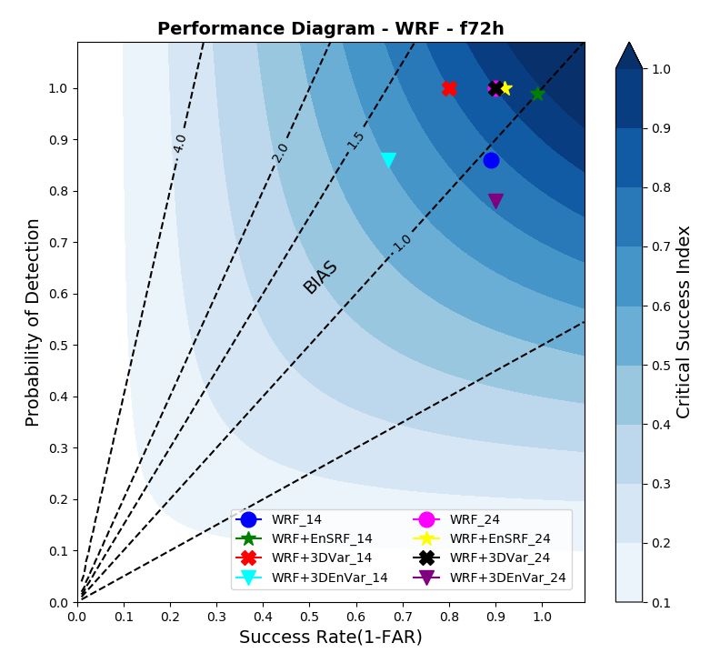
Atmosphere 2021, 12, 1201                                                                                            7 of 20

                            which in turn are calculated as the difference between each ensemble member (n) and the
                            ensemble mean. Pb is given in Equation (8), as shown in [37].
                                                                                n
                                                                        1             0   0
                                                             Pb =
                                                                    ( n − 1)   ∑ xnb (xnb )T                            (8)
                                                                               i =1

                            2.5.4. Three-Dimensional Ensemble-Variational
                                 In the 3DEnVar, the model error covariance matrix (B) is a linear combination of
                            the static matrix of 3DVar (B3DVar ) and the one updated by the EnSRF (Pb ), as shown in
                            Equation (9). At the end of the analysis step, the 3DEnVar cost function is minimized by
                            using the hybrid background error covariance matrix using the linear combination of the
                            matrices, as shown in Equation (9).

                                                              B = (1 − α)B3DVar + αPb                                   (9)
                                 In Equation (9), α is the coefficient used to weigh the contribution of the two matrices.
                            This work used the optimal weights of 0.75 for EnSRF and 0.25 for 3DVar.
                                 The RMS version used in this work tested the settings for a hybrid assimilation system
                            with weights for the ensemble background error covariance of 50, 75, and 100%, trying
                            to reproduce the same experiment of very short-term weather forecasts Rapid Refresh,
                            RAP [38]. Based on the single observation test, the best analyses results were with an
                            ensemble background error covariance of 75%, similar to the results of [38]. With the
                            weight of 75%, the analyses increment have fields influencing more grid points in the
                            horizontal and vertical, contributing to the matrix taking its contribution to more grid
                            points away from the observation location.

                            2.6. Statistical Data Analysis
                                  The contingency table indexes (Equations (10)–(14)) plotted in a performance diagram
                            were used to show the WRF 24 h accumulated precipitation forecast performance by
                            using initial conditions updated by 3DVar, EnSRF, and 3DEnVar. They evaluated the WRF
                            performance for all experiments over the Maranhão state surface meteorological stations
                            (Figure 2), which is the region where MCS occurred.
                                  In order to quantify the Probability of Detection (POD), False Alarms (FAR), errors, and
                            hits, the contingency table [39] was calculated and described by Equations (10) and (11),
                            respectively. The FAR and POD range from 0 to 1. The FAR index has better performances
                            when its value is closer to 0, while the POD indicated better performances when its value
                            was closer to 1.
                                                                            false alarm
                                                               FAR =                                                   (10)
                                                                        false alarm + hits
                                                                              hits
                                                                POD =                                                 (11)
                                                                         hits + errors
                                  Another method for evaluating the performance of a given estimate is to calculate the
                            Success Rate (SR) obtained by the ratio of the number of hits by the total number of hits
                            plus false alarms, as shown in Equation (12). Thus, for values close to one, the estimate
                            is accurate.
                                                                           hits
                                                            TS =                                                   (12)
                                                                   hits + false alarm
                                 The frequency BIAS (Equation (13)) shows the relationship between the number of
                            estimated events and the number of observed events. The calculation results will return
                            values greater than zero. Values closer to one indicate better performances, and values
                            greater than or less than one indicate that the occurrence of events was, respectively,
                            overestimated and underestimated.
                                                                       false alarm + hits
                                                             BI AS =                                                  (13)
                                                                          hits + errors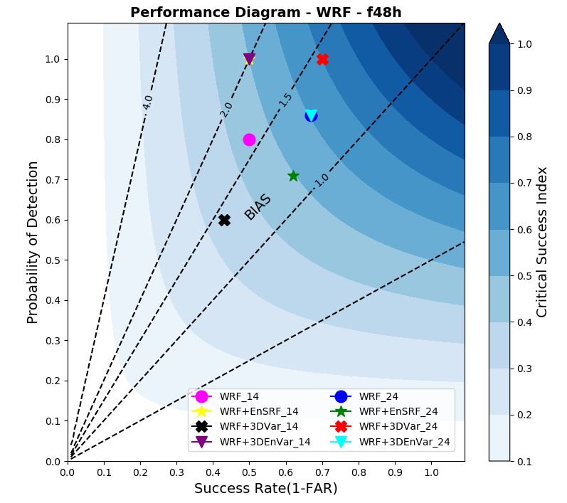
Atmosphere 2021, 12, 1201                                                                                           8 of 20

                                 The Critical Success Index (CSI) was calculated (Equation (14)) for the accumulated
                            rainfall estimates obtained from different data sources. By using the CSI, it is possible
                            to observe the percentage of correct answers, deducting the number of times that the
                            non-occurrence of events correctly predicted the events. Values close to one indicate
                            good performances.
                                                                           hits
                                                        CSI =                                                    (14)
                                                               false alarm + hits + errors
                                 The Root Mean Square Error (RMSE), Equation (15)) also showed how the 24 h
                            accumulated precipitation from the WRF model is distant from the observational data and
                            the accuracy of the model data. In order to conduct this, it was necessary to use the surface
                            meteorological stations over Maranhão as the references.
                                                                 v                             !
                                                                              N
                                                                 u
                                                                         1
                                                                             ∑ (xi − yo
                                                                 u
                                                          RMSE = t                        )2                          (15)
                                                                         N   i =1

                            Figure 2. The map represents the topography (m) and the INMET meteorological stations over
                            Maranhão state (red circles).

                            3. Results and Discussion
                            3.1. Convective Rainfall
                                 The intense rain episodes on the BNE, evaluated in this study, occurred on 14th and
                            24th January 2017 in the cities of Barra da Corda (5.51◦ S and 45.24◦ W) and Colinas (6.03◦
                            S and 44.23◦ W), respectively. Both cities are in the most continental portion of the state of
                            Maranhão, as illustrated in Figure 2.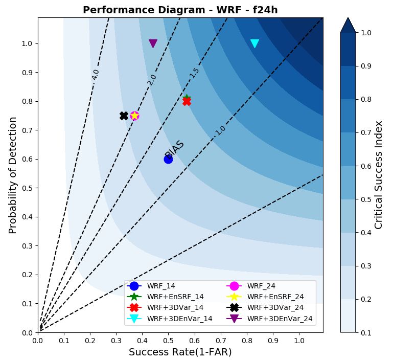
Atmosphere 2021, 12, 1201                                                                                           9 of 20

                                 The MCS1 (the event that took place on 14 January 2017) covered a total surface area
                            of 218,000 km2 , during the maximum development stage, with cloud top temperatures
                            below −80 ◦ C. This system caused heavy rain events mainly over the central region of
                            Maranhão, around 6◦ S and 46◦ W, where rainfall accumulated in 24 h recorded by the
                            conventional INMET station in Barra da Corda (MA) was equivalent to 72.5 mm (Figure 3).

                            Figure 3. MERGE 24 h accumulated precipitation over the BNE (mm) for the MCS1 event.

                                 Referring to Figure 3, it is possible to observe an area with intense daily rain episodes
                            over the state of Maranhão greater than 50 mm. This region was under the influence of
                            a convective systems, and it caused the heavy rain (greater than 70 mm) reported by the
                            INMET surface meteorological station in the Barra da Corda region (6◦ S and 46◦ W).
                                 For 24 January 2017, the daily accumulated rainfall field obtained from MERGE
                            (Figure 4) is illustrated over the city of Colinas (6◦ S and 44◦ W), with precipitation above
                            50 mm for the area of influence of the MCS.
                                 The MCS2 (the event that took place on 24 January 2017) covered a total surface area
                            of 143,000 km2 during the maximum development stage, with cloud top temperatures
                            below −80 ◦ C. This system caused heavy rain events recorded by INMET surface stations
                            (equal to 72 mm) over the central-east region of Maranhão.
                                 Thus, for the two days with records of heavy rains over the cities in the Maranhão
                            state, MERGE estimates indicated a large volume of rain (around 75 mm), proving to be a
                            particularly effective product in the characterization of precipitation accumulated in 24 h
                            during episodes of MCS over BNE that occurred on 14th and 24th January 2017.
Atmosphere 2021, 12, 1201 10 of 20
Figure 4. MERGE 24 h accumulated precipitation over the BNE (mm) for the MCS2 event.
3.2. Total of Assimilated Data
In general, the number of observations used during the DA procedure for pressure,
specific humidity, temperature, and wind speed was similar to those presented in Figure 5
along with DA cycles. The assimilated data in both MCS are similar and both present large
amounts of wind data due to the availability of Atmospheric Motion Vectors (AMV) data,
obtained from satellite observations.
Unfortunatelly, the limited availability of conventional meteorological data in the
northeast region of Brazil may affect the performance of the DA, which can result in a
lower skill of the WRF forecasts.
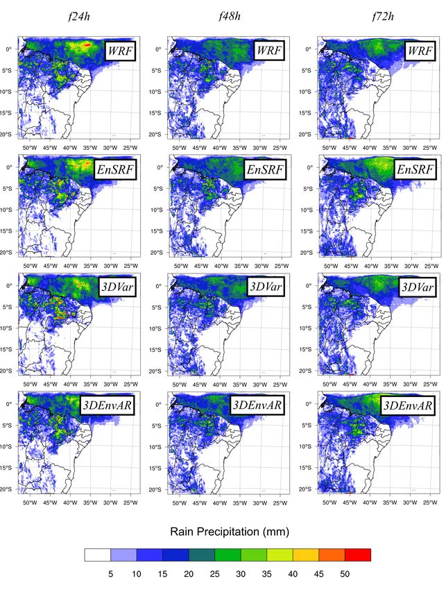
3.3. WRF 24-h Accumulated Precipitation
The predictions performed by the WRF model regarding 24 h accumulated rainfall for
14th January 2017 (Figure 6) reveal that, in general, all the experiments were able to produce
rainfall events superior to 5 mm over the region of Barra da Corda (6◦ S and 45◦ W), in
Maranhão.The WRF forecasts have spatial distributions similar to the 24 h accumulated
rain fields obtained from the MERGE (Figure 3).
Despite the similarity between the MERGE 24 h rainfall fields, the predictions of the
f24h experiment (Figure 6), in general, present a large area covering the state of Maranhão,
with daily rainfall accumulations superior to 5 mm, when using the initial conditions of
GEFS, EnSRF, and 3DEnVar, respectively, to the f24h-WRF, f24h-EnSRF, and f24h-3DEnVar
experiments (Figure 6). Otherwise, the precipitation data from the WRF model initialized
with the 3DVar analysis (experiment f24-3DVar, in Figure 6) presented a drier atmosphere
(with fewer precipitation areas greater than 5 mm covering the state of Maranhão compared
with the others experiments) for f24h-WRF, f24h-EnSRF, and f24h-3DEnVar (Figure 6). As aAtmosphere 2021, 12, 1201 11 of 20
result, f24h-3DVar (Figure 6) had an inferior performance when compared with the others
experiments.
Figure 5. Number of observations of surface pressure (P, in Pa), temperature (T, in K), specific
humidity (Q, in g/kg), and zonal and meridional wind speed (UV, in m/s) assimilated in the GSI on
12 (MCS1) and 22 (MCS2) January 2017, at 0000 UTC.
Figure 7 shows the RMSE of 24, 48, and 72 h forecast among the experiments evaluated
on 14th January 2017. The f24h-3DVar had the worst performance compared to f24h-WRF,
f24h-EnSRF, and f24h-3DEnVar. Thus, the model errors compared with INMET observa-
tions on the state of Maranhão were around 22 mm for the f24h experiments (WRF, EnSRF,
and 3DEnVar), and the model error was greater than 25 mm in the f24h-3DVar. Among
the many reasons for the f24h-3DVar’s lower performance was the 3DVar static covariance
matrix of forecast errors in time. Therefore, the model errors represented by this matrix
may not represent the errors of the fields represented in the background for the whole year
or in the MCS presence in the tropical region, which can result in rainfall forecasts that
differ from the observations. The justification is because the numerical weather prediction
models are sensitive to initial conditions, and any errors in initial conditions make a few of
weather predictions performed by the WRF model equations reliable.Atmosphere 2021, 12, 1201 12 of 20
Figure 6. The 24 (f24h), 48 (f48h), and 72 h (f72h) hours forecast relative to WRF 24 h rain precipitation over the BNE (mm)
for the SMC1 event, without initial conditions updated by GSI (WRF), and the initial conditions updated by the EnSRF,
3DVar, and 3DEnVar GSI algorithm.Atmosphere 2021, 12, 1201 13 of 20
Figure 7. The 24 (f24h), 48 (f48h), and 72 (f72h) hours forecast relative to the WRF RMSE of forecasted
24 h accumulated precipitation over the BNE (mm) for the SMC1 event, without initial conditions
updated by GSI (WRF), and the initial conditions updated by the EnSRF, 3DVar, and 3DEnVar
GSI algorithm.
The best 24 h WRF precipitation performance accumulated rainfall field was for the
experiments Figure 7-f24h-3DEnVar and f24h-EnSRF. Note in Figure 7, that the forecast
errors obtained in these configurations are around 22 mm, the smallest among the experi-
ments. The good RMSE performances illustrated in Figure 7-f24h-3DEnVar and f24h-EnSRF
occurred because the analysis in EnSRF and 3DEnVar uses the background error covariance
matrix to update the initial conditions with the error of the day. Thus, this matrix updates
at each assimilation cycle with the error of the day calculated from ensemble forecast
members, as shown in Equation (8). The ensemble methodology contributes to obtaining
initial conditions that minimize the systematic errors of the background used in DA and
contributes to rainfall forecasts closer to those observed in meteorological stations.
The best WRF model predictions for f48h and f72h experiments (Figure 6) used 3DEn-
Var analyses, for which its forecast errors regarding INMET meteorological observations
on the state of Maranhão were around 23 mm for both experiments. Otherwise, the WRF
forecast model initialized with the 21 EnSRF analyses (for the f48h and f72h experiments)
obtained the worse RMSE values from the experiment, with errors superior to 25 mm
in both experiments (Figure 7). This performance of the WRF model initialized with the
EnSRF analyses suggested that ensemble predictions used to obtain the EnSRF background
error covariance matrix were very small. Thus, the limited ensemble member numbers
represent a small ensemble of atmospheric conditions, which resulted in an EnSRF matrix
with a low potential for representing the atmospheric model errors in the experiment and
an increase in forecast errors.
In summary, among the evaluated experiments, the one that presented the best perfor-
mance in the 24 h rainfall accumulated forecast for 14 January 2017 was the WRF model
started with the 3DEnVar analyses. Therefore, on 14 January 2017, the hybrid matrix of
3DEnVar contributed to minimizing the rain forecast errors.
The WRF model predictions for 24 January 2017 (Figure 8) illustrate that, for all
experiments, it was possible to predict rainfall events with a threshold greater than 5 mm
over the Colinas region (6◦ S and 44◦ W) where the MCS episode took place. Furthermore,
a simple comparison shows a similar spatial distribution of the MERGE 24 h accumulated
rainfall field, and it is represented by the different predictions of the WRF model depicted
in Figure 8. However, in general, the predicted values underestimated the daily rainfall
obtained by MERGE.Atmosphere 2021, 12, 1201 14 of 20
Figure 8. RMSE of 24 h accumulated precipitation (mm) started at 24 (f24h), 48 (f48h), and 72 h (f72h)
before SMC2 event day over the BNE (mm), without initial conditions updated by GSI (WRF), and
the initial conditions updated by EnSRF, 3DVar, and 3DEnVar GSI algorithm.
The MERGE 24 h accumulated rainfall fields show a similar distribution of precipita-
tion over the BNE, as illustrated in Figure 8. The RMSE showing a notorious difference
between analysis and the INMET meteorological observations on the Maranhão state is
in the Figure 8-f24h-WRF experiment. For this experiment, the errors can be as great as
35 mm.
The best WRF forecast performance started 24 h before the SCM2 was the experiment
f24h-EnSRF (Figure 9). The experiment f48h-EnSRF also had small forecast errors when
compared with INMET meteorological stations. Thus, in the Figure 9-f24h-EnSRF and
f48h-EnSRF experiments, a set of predictions initialized with analysis from the EnSRF that
obtained a small prediction error of f24h and f48h experiments is portrayed, as shown by
the RMSE value around 28 mm.Atmosphere 2021, 12, 1201 15 of 20
Figure 9. The 24 (f24h), 48 (f48h), and 72 (f72h) hours forecast relative to WRF RMSE of forecasted 24 h
accumulated precipitation over the BNE (mm) for the SMC2 event, without initial conditions updated
by GSI (WRF), and the initial conditions updated by the EnSRF, 3DVar, and 3DEnVar GSI algorithm.
The worst performance of the f48h experiment was obtained by the WRF model
initialized with the 3DVar analysis, with an error of 35 mm referring to the RMSE (Figure 9).
As discussed previously in this section, the 3DVar static background error covariance
matrix may be one of the source of this lower skill. The static matrix may not represent
accuracy systems such MCS2, and the introduction of the errors of the day by the ENSRF
or 3DEnVar improves the representations of this system.
In the f72h experiment, initialized with the 3DVar, EnSRF, and 3DEnVar analyses, the
errors were superior (around 33 mm) to the WRF model errors initialized with the GEFS
analysis, with values referring to the RMSE around 28 mm (Figure 9). This situation may
be due to the fact that the analysis fields generated in the RMS through 3DVar, EnSRF, and
3DEnVar were not able to minimize the background errors when updating the analyses.
The Figure 9-f72h-WRF experiment used the GEFS control member as an initial
condition. As this control member is from a DA system used by the NCEP for the generation
of analysis (the EnSRF), the results obtained in the f72h-WRF experiment performed well.
This is in part attributed to the initial conditions obtained from the EnSRF, which were able
to reduce background errors and consequently helped the WRF model in obtaining better
performance in rainfall forecast compared to the other experiments evaluated in Figure 8.
In summary, for the predictions of the WRF model valid for 24th January 2017, the
importance of DA by set in the best performance of the WRF model initialized with GEFS
and EnSRF is noted. The lower WRF model performance initialized with the 3DVar and
3DEnVar analyses suggests a deficiency of the static background error covariance matrix in
correcting the forecast errors. This deficiency could be diminished by assigning a higher
weight to the EnSRF covariance matrix in 3DEnVar and/or by obtaining a new static matrix.
3.4. WRF Rainfall Forecast by Performance Diagram
The performance diagram for the 24 h accumulated precipitation from the WRF model
initialized 24 h in advance (MCS1 and MCS2) illustrates that the probability of detection
(POD) for events with a higher threshold of 5 mm forecasted by the WRF model initialized
with 3DEnVar analysis was the highest value among the evaluated experiments Figure 10
(POD equivalent to 100%). Likewise, by the diagram shown in Figure 10, the success rate of
the WRF experiments initialized with 3DEnVar analysis performed satisfactorily, reaching
a success rate equivalent to 80%, the highest among the evaluated experiments. This fact
demonstrates that the predictions of the WRF experiment having the 3DEnVar analysisAtmosphere 2021, 12, 1201 16 of 20
as an initial condition performed well in terms of the rainfall accumulated in 24 h for a
threshold greater than 5 mm.
Figure 10. Performance diagram for the WRF model daily rainfall initialized with GEFS and the
initial conditions of EnSRF, 3DVar, and 3DEnVar for the 14th and 24th January 2017, initialized
24 h earlier.
The frequency BIAS of the performance diagram, Figures 10 and 11, illustrates that
WRF experiments generated by one of the evaluated DA systems, in general, overestimated
the meteorological observations, as well as the predictions of the WRF model initialized
with the GEFS control member.
Similarly to the daily accumulated rainfall performed by the WRF model that was
started 24 h earlier with the initial conditions of 3DEnVar, the forecasts started 48 h earlier
with the same settings and managed to return a high POD for the rain events equivalent to
100%. It was the best result among the evaluated experiments (Figure 11). The analysis
updated by 3DEnVar also had a good performance associated with the success rate (greater
than 60%). This finding revealed that this configuration also performed well in detecting
the absence of rain when the INMET surface stations did not register rain.
The forecast of accumulated rainfall in 24 h of the WRF model started 72 h earlier
with 3DEnVar analysis (Figure 12) showed a POD greater than 70% for the days of intense
rain occurrence over the Maranhão state. Despite this fact, they did not have the best
performance among the evaluated configurations regarding POD, which for the other
experiments (WRF, 3DVar, and EnSRF) were superior to 80%. The success rate for the
predictions updated by the 3DEnVar initial conditions performed the same as verified in
the previous experiments. The success rate values were superior to 60% when the predicted
values, as illustrated by the frequency BIAS (Figure 12), overestimated the observations
and underestimated the accumulated rainfall observed on 14th and 24th January 2017,
respectively.Atmosphere 2021, 12, 1201 17 of 20
Figure 11. Performance diagram for the WRF model daily rainfall initialized with GEFS and the
initial conditions of EnSRF, 3DVar, and 3DEnVar, for 14 and 24 January 2017, initialized 48 h earlier.
Figure 12. Performance diagram for the WRF model daily rainfall initialized with GEFS and the
initial conditions of EnSRF, 3DVar, and 3DEnVar, for 14 and 24 January 2017, initialized 72 h earlier.
The best performances obtained in the 24 h accumulated rain forecast were from
the WRF model initialized with the 3DEnVar analysis on the points of the meteorological
station of INMET, on the state of Maranhão, as depicted by calculating the contingency
table indices and reference [16]. Thus, the best performance of the WRF model for the 24Atmosphere 2021, 12, 1201 18 of 20
and 48 h forecasts using the initial conditions updated by 3DEnVar occurred due to the
combination of the analysis updated by 3DEnVar with the errors of the day and the WRF
parameterizations adopted for forecasting. Therefore, the best performance of the WRF
model for 24 and 48 h forecast using the initial conditions updated by 3DEnVar occurred
due the combination of the analysis updated by 3DEnVar with the errors of the day and
the WRF parameterizations adopted for forecasting.
Another interesting fact is that the metrics in Figures 10–12 show that the best per-
formances of the model were proportional to the increase in the length of the forecast
(note the BIAS, SR, POD, and FAR best performances in different SMR settings). This
finding occurred due to spin-up length (time required for the model to reach its internal
equilibrium). Typically, short-term weather forecast models require a 6–12 h spin-up [40].
Nonetheless, none of the forecasts carried out with the analysis of DA systems are
evaluated here, and experiments without initial conditions updating indicated the possibil-
ity of heavy rain as registered by meteorological stations was only of moderate intensity.
One justification is the bad performance of the WRF Cumulus parametrization. In this
work, they were chosen based on the [23] work, while another work suggests Kain–Fritsch
as the best parametrization for the Brazilian Northeast region [41].
Encouraging results have been obtained in several works over the years by using
hybrid assimilation 3DEnVar based on EnSRF and 3DVar. The results presented in these
works [16,38] and this study case show that 3DEnVar is an efficient algorithm for improving
rainfall forecasts for its study locations. This fact occurs because 3DEnVar updates the
analyses with the errors of the day, decreasing the initial condition errors that affect the
weather forecast performed by the WRF equations.
4. Conclusions
This work evaluated the 3DVar, the EnSRF, and the 3DEnVar DA impact in the
generation of analyses in order to verify their contributions in the heavy rain forecasts in the
BNE. We concluded that the inclusion of the errors of the day in the 3DVar (climatological)
backgound covariance matrix, i.e, by using the EnSRF and the 3DEnVar, the analysis was
improved and it led to a better precipitation forecast.
Throught the RMSE evaluation, we concluded that the WRF model initialized with
the initial conditions from 3DEnVar (experiments f24h, f48h, and f72h) for the MCS1
and from EnSRF (24h and f48h experiments) and GEFS (experiment f72h) for the MCS2
(2017) produced the best forecasts. In general, these results shows that the errors of the day
considered in the EnSRF and the hybrid ensemble variational background error covariances
improved the WRF forecasts.
The contingency table indices also revealed that the WRF model initiated with the
3DEnVar analysis also improved its ability to detect rainfall for different regions in the
Maranhão state. However, the heavy rainfall events associated with the MCS over the
BNE were underestimated for all evaluated experiments (considering the 24 h accumulated
precipitation). The employed cumulus cloud parameterization scheme may have limita-
tions on forecasting heavy rain associated with MCS in the BNE, since all experiments
underestimated the heavy precipitation.
The lack of enough conventional temperature, humidity, and pressure data available
for being assimilated in the BNE may also have impacted the quality of the model’s
predictions, despite the best performance of the WRF model initiated with 3DEnVar in
SCM1 and with EnSRF in SCM2.
In summary, the results showed that 3DEnVar could improve the WRF 24 h accu-
mulated precipitation forecast, as shown with the MCS1. However, the MCS2 evaluation
showed that the WRF model initialized with the EnSRF analysis had better results. There-
fore, in order to improve the predictions through the WRF model by considering the
3DEnVar, some solutions are as follows: to create an algorithm that automatically defines
the weights assigned to the EnSRF and 3DVar covariance matrix in the GSI hybrid sys-
tem; an increase in the ensemble size; an increase in model resolution (horizontal andAtmosphere 2021, 12, 1201 19 of 20
vertical); and an increase in the ensemble state by using some ensemble of model physical
parametrizations.
Author Contributions: Conceptualization, J.P.G.N.; Methodology, É.P.V. and C.F.B.; Software, J.P.G.N.,
É.P.V. and C.F.B.; Formal analysis, J.P.G.N.; Investigation, J.P.G.N.; Data curation, J.P.G.N.; Writing—
original draft preparation and review/editing, J.P.G.N., É.P.V., and C.F.B.; Supervision, É.P.V. and
C.F.B. All authors have read and agreed to the published version of the manuscript.
Funding: This study was financed in part by the Coordenação de Aperfeiçoamento de Pessoal de
Nível Superior-Brasil (CAPES)-Finance Code 001. J.P.G.N was supported by the National Council for
Scientific and Technological Development (CNPq).
Acknowledgments: The authors thank CAPES and CNPq for the finantial support and INPE/PGMET
for the computational infrastructure for developing this study.
Conflicts of Interest: The authors declare no conflict of interest.
Abbreviations
The following abbreviations are used in this manuscript:
3DEnVar 3D Ensemble Variational;
3DVar 3D Variational;
BNE Brazilian Northeast;
CSI Critical Success Index;
DA Data Assimilation;
EnSRF Ensemble Kalman Filter;
FAR False Alarm;
POD Probability of Detection;
MCS Mesoscale Convective System;
RMS Regional Modeling System;
RMSE Root Mean Square Error;
SR Success Rate;
WRF Weather Research and Forecasting;
GSI Grid Statistical Interpolation.
References
1. Confederação Nacional dos Municípios. Available online: https://www.cnm.org.br (accessed on 4 January 2021).
2. Meteored. Available online: https://www.tempo.com/ (accessed on 2 January 2021).
3. Brasseur, P. Ocean data assimilation using sequential methods based on the Kalman filter. Ocean Weather Forecast. 2006, 271–276.
[CrossRef]
4. Gilchrist, B; Cressman, G.P. An Experiment in Objective Analysis. Tellus 1953, 6, 310–318.
5. Kalnay, E. Atmospheric Modeling, Data Assimilation and Predictability, 1st ed.; Cambridge University Press: New York, NY, USA,
2002; pp. 1–341.
6. Panofsky, R.A. Objective weather-map analysis. J. Meteorol. 1949, 6, 386–392. [CrossRef]
7. Bergthórsson, P.; Doos, B.R. Numerical weather map analyses. Tellus 1955, 7, 329–340. [CrossRef]
8. Cressman, G.P. An operational objective analysis system. Mon. Weather Rev. 1959, 7, 367–374. [CrossRef]
9. Eliassen, A. Provisional report on calculation of spatial covariance andautocorrelation of the pressure field. Weather Clim. 1954, 5, 1–10.
10. Gandin, L.S. The objective analysis of meteorological fields: Israel program for scientific translatinons. Hydrometeoro Press 1963,
5, 1–10.
11. Sasaki, Y. Some basic formalisms in numerical variational analysis. Mon. Weather Rev. 1970, 98, 875–883. [CrossRef]
12. Flaterry, T. Spectral models for global analysis and forecasting. Air Weather Serv. Tech. 1970, 242, 42–54.
13. Talagrand, O. Assimilation of Observations, an Introduction. J. Meteorol. Soc. Jpn. Ser. II 1997, 75, 191–209. [CrossRef]
14. Li, Y.; Wang, X.; Xue, M. Assimilation of Radar Radial Velocity Data with the WRF Hybrid Ensemble–3DVAR System for the
Prediction of Hurricane Ike (2008). Mon. Weather Rev. 2012, 140, 3507–3524. [CrossRef]
15. Gao, J; Stensrud, D.J. Some Observing System Simulation Experiments with a Hybrid 3DEnVAR System for Storm-Scale Radar
Data Assimilation. Mon. Weather Rev. 1963, 142, 3326–3345.
16. Bastarz, A.B. Assimilação de Dados Global Híbrida por Conjunto-Variacional no CPTEC. Ph.D. Thesis, National Institute for
Aerospace Studies, São José dos Campos, Brazil, 2017.
17. Lyra, M.J.A.; Freitas, I.G.F. Desenvolvimento dos Complexos Convectivos de Mesoescala no Nordeste Brasileiro em 2017. Rev.
Bras. Geogr. Física 2019, 2, 2152–2162. [CrossRef]Atmosphere 2021, 12, 1201 20 of 20
18. Machado, L.A.T.; Laurent, H. The convective system area expansion over Amazônia and its relationships with convective system
life duration and high-level wind divergence. Mon. Weather Rev. 2004, 132, 714–725. [CrossRef]
19. Rozante, J.R.; Moreira, D.S.; Gonçalves, L.G.G.; Vila, D.A. Combining TRMM and Surface Observations of Precipitation: Technique
and Validation over South America. Weather Forecast. 2010, 25, 885–894. [CrossRef]
20. Powers, J.G.; Klemp, J.B.; Skamarock, W.C.; Davis, C.A.; Dudhia, J.; Gill, D.O.; Coen, J.L.; Gochis, D.J. The weather research and
forecasting model: overview, system efforts, and future directions. Bull. Am. Meteorol. Soc. 2017, 98, 1717–1737. [CrossRef]
21. Institute of Airspace Control. Available online: http://pesquisa.icea.gov.br/ (accessed on 6 July 2014).
22. Nobre, J.P.G.; Fedorova, N.; Levit, V.; Santos, A.S.; Lyra, M.A. New Methodology for Evaluation of the Fog Events for the Zumbi
dos Palmares Airport, in Maceió (Alagoas). Anuário Inst. Geociências-UFRJ 2019, 42, 527–535. [CrossRef]
23. Sun, B.Y.; Bl, X.Q. Validation for a tropical belt version of wrf: sensitivity tests on radiation and Cumulus convection parameteri-
zations. Atmos. Ocean. Sci. Lett. 2019, 12, 192–200. [CrossRef]
24. Zhang, C.; Wang, Y. Projected future changes of tropical cyclone activity over the western north and south pacific in a 20-km-mesh
regional climate model. J. Clim. 2017, 30, 5923–5941. [CrossRef]
25. Tiedtke, M.A. A comprehensive mass flux scheme for Cumulus parameterization in larger- scale model. Montly Wearther Rev.
1989, 117, 1779–1800. [CrossRef]
26. Kain, S.J. The kain—fritsch convective parameterization: An update. J. Appl. Meteorol. Climatol. 2004, 42, 170–181. [CrossRef]
27. Han, J.; Pan, H.L. Revision of convection and vertical diffusion schemes in the NCEP global forecast system. Weather Forecast.
2011, 26, 520–533. [CrossRef]
28. DOC/NOAA/NWS/NCEP/EMC > Environmental Modeling Center, National Centers for Environmental Prediction, National
Weather Service, NOAA, U.S. Department of Commerce. Available online: https://www.ncei.noaa.gov/access/metadata/
landing-page/bin/iso?id=gov.noaa.ncdc:C00691 (accessed on 25 August 2021).
29. NASA Shuttle Radar Topography Mission (SRTM). Shuttle Radar Topography Mission (SRTM) Global. Distributed by OpenTo-
pography. 2013. Available online: doi:10.5069/G9445JDF (accessed on 25 August 2021).
30. Atmospheric and Environmental Research. Available online: http://rtweb.aer.com (accessed on 4 January 2021).
31. Hong, S.; Lim, J. The WRF single-moment 6-class microphysics: Song-you hong. J. Korean Meteorol. Soc. 2006, 2, 129–151.
32. Hong, S.-Y.; Noh, Y.; Dudhia, J.A. New vertical diffusion package with an explicit treatment of entrainment processes. Mon.
Weather Rev. 2006, 134, 2318–2341. [CrossRef]
33. Tewari, M.F.; Chen, W.; Wang, J.; Dudhia, M.A.; Lemone, K.; Mitchell, M.E.; Gayno, G.; Wegiel, J.; Cuenca, R.H. Implementation
and verification of the unified NOAH land surface model in the WRF model. In Proceedings of the Conference on Weather
Analysis and Forecasting, Seattle, WA, USA, 10 January 2004; pp. 11–15.
34. Parrish, D.F.; Derber, J.C. The National Meteorological Center’s Spectral Statistical-Interpolation Analysis System. Mon. Weather
Rev. 1992, 120, 1747–1763. [CrossRef]
35. Bierman, G. Factorization Methods for Discrete Sequential Estimation, 1st ed.; Academic Press: New York, NY, USA, 1977; pp. 1–241.
36. Maybeck, P.S. Stochastic Models, Estimation, and Control, 1st ed.; Academic Press: New York, NY, USA, 1983; pp. 1–423.
37. Developmental Testbed Center. Available online: https://dtcenter.ucar.edu/com-GSI/users/docs/ (accessed on 18 January 2021).
38. Hu, M.; Benjamin, S.G.; Ladwig, T.T.; Dowell, D.C.; Weygandt, S.S.; Alexander, C.R.; Whitaker, J.S. GSI Three-Dimensional
Ensemble–Variational Hybrid Data Assimilation Using a Global Ensemble for the Regional Rapid Refresh Model. Mon. Weather
Rev. 2017, 145, 4205–4225. [CrossRef]
39. Da Paz, A.R.; Collischonn, W. Avaliação de estimativas de campos de precipitação para modelagem hidrológica distribuída. Rev.
Bras. Meteorol. 2011, 26, 109–120. [CrossRef]
40. Skamarock, W.C. Evaluating Mesoscale NWP Models Using Kinetic Energy Spectra. Mon. Weather Rev. 2004, 132, 3019–3032.
[CrossRef]
41. Dantas, V.A.; Silva Filho, V.P.; Santos, E.B.; Gandu, A.W. Testando diferentes esquemas da parametrização cumulus do modelo
WRF, para a região norte Nordeste do Brasil. Rev. Bras. Geogr. Física 2019, 12, 754–767. [CrossRef]You can also read


