Music source separation conditioned on 3D point clouds
←
→
Page content transcription
If your browser does not render page correctly, please read the page content below
Music source separation conditioned on 3D point
                                        clouds
                                                 Francesc Lluı́s,a Vasileios Chatziioannou, and Alex Hofmann
                                                 Department of Music Acoustics, University of Music and Performing Arts Vienna, Austria
                                                 (Dated: 4 February 2021)
                                                 Recently, significant progress has been made in audio source separation by the application of
                                                 deep learning techniques. Current methods that combine both audio and visual information
                                                 use 2D representations such as images to guide the separation process. However, in order
                                                 to (re)-create acoustically correct scenes for 3D virtual/augmented reality applications from
                                                 recordings of real music ensembles, detailed information about each sound source in the
                                                 3D environment is required. This demand, together with the proliferation of 3D visual
                                                 acquisition systems like LiDAR or rgb-depth cameras, stimulates the creation of models that
arXiv:2102.02028v1 [cs.SD] 3 Feb 2021

                                                 can guide the audio separation using 3D visual information. This paper proposes a multi-
                                                 modal deep learning model to perform music source separation conditioned on 3D point
                                                 clouds of music performance recordings. This model extracts visual features using 3D sparse
                                                 convolutions, while audio features are extracted using dense convolutions. A fusion module
                                                 combines the extracted features to finally perform the audio source separation. It is shown,
                                                 that the presented model can distinguish the musical instruments from a single 3D point
                                                 cloud frame, and perform source separation qualitatively similar to a reference case, where
                                                 manually assigned instrument labels are provided.
                                                 ©2021 Acoustical Society of America.         [https://doi.org(DOI number)]

                                                 [XYZ]                                                                            Pages: 1–10

                                        I. INTRODUCTION                                               fusion strategies12 have been studied. In addition, other
                                                                                                      methods learning also from motion representation, such
                                            The task of recovering each audio signal contribu-        as low-level optical flow13 or keypoint-based structured
                                        tion from an acoustic mixture of music has been actively      representation14 , have been proposed to facilitate the
                                        explored throughout the years1 and significant progress       model to separate simultaneously musical sources com-
                                        has been made recently using deep learning methods2–5 .       ing from the same type of instrument.
                                        Although music source separation has been tradition-               The proliferation of 3D visual acquisition systems
                                        ally tackled using only audio signals, the emergence of       such as LiDAR and various rgb-depth cameras in de-
                                        data-driven techniques has facilitated the inclusion of       vices used in a day-to-day fashion allows to easily cap-
                                        visual information to guide models in the audio sep-          ture 3D visual information of the environment. This,
                                        aration task. Music source separation conditioned on          together with their capability to record audio, stimulates
                                        visual information has also gained significant improve-       the development of algorithms that can learn from 3D
                                        ment through the application of deep learning models6 .       video along with audio and opens new possibilities for
                                        The proposed deep learning methods mainly use appear-         virtual reality (VR) and augmented reality (AR) appli-
                                        ance cues from the 2D visual representations to condi-        cations. Audio is crucial to bring meaningful experiences
                                        tion the separation. Gao et al.7 proposed a two step          to people in VR/AR applications. VR/AR applications
                                        procedure, where initially a neural network learns to as-     are meant to be a multimodal and interactive experi-
                                        sociate audio frequency bases with musical instruments        ence where the sound perception has to be convincing
                                        appearing in a video. Then, the learned audio bases           and match the other sensory information perceived. A
                                        guide a non-negative matrix factorization framework to        first step to render proper acoustic stimuli for VR/AR
                                        perform source separation. Concurrently, Zhao et al.8         applications is to know the sound of each object in the
                                        proposed PixelPlayer, a method capable to jointly learn       3D environment15 . When scanning and recording an en-
                                        from audio and video to perform both source separation        vironment, multiple sources emit sound simultaneously
                                        and localization. Since then, source separation models        and therefore, source separation algorithms are needed
                                        conditioned on visual information have been enhanced          to separate the audio and associate it to each source in
                                        with different approaches such as using recursivity9 or       the 3D environment.
                                        co-separation loss10 . Recently the importance of appear-          In this paper, we propose a model for source separa-
                                        ance cues for music source separation11 and multi-modal       tion conditioned on 3D videos, i.e. sequences of 3D point
                                                                                                      clouds, an approach which appears to be unexplored. For
                                                                                                      clarity of exposition, the deep learning model learns to
                                        a lluis-salvado@mdw.ac.at                                     separate individual sources from a musical audio mixture

                                        J. Acoust. Soc. Am. / 4 February 2021                                                         Music source separation   1
given the 3D video associated with the source of inter-      the mix-and-separate approach consists of generating
est. The model consists of a 3D video analysis network       artificial audio mixtures via mixing individual sound
which uses sparse convolutions to extract visual features    sources. Then, the learning objective is to recover each
from the 3D visual information and an audio network          individual sound source conditioned on its associated
with dense convolutions that extracts audio spectral fea-    visual information. This allows to use unlabeled indi-
tures from an audio mixture spectrogram. Finally, an         vidual sounds itself as supervision. Therefore, although
end module leverages the multimodal extracted features       the network is trained in a supervised fashion, the whole
to perform source separation. 3D visual representations,     pipeline is considered self-supervised.
as opposed to 2D representations, allow to access the lo-         Music source separation conditioned on 3D visual in-
cation of the sources in space and therefore exploit the     formation is a new domain. While there are lots of au-
distance between each source and the receiver for further    dio datasets18 , there is data scarcity of 3D videos from
auralization purposes15 . However, unlike 2D visual rep-     musicians. For the purposes of this work, we capture
resentations which are represented in a dense grid, 3D       3D videos of several performers playing five different in-
representations are very sparse and the surface of the       struments: cello, doublebass, guitar, saxophone, and vi-
captured objects are represented as a set of points in the   olin. In addition, we separately collect audio recordings
3D space which adds the additional difficulty when ex-       for these instrument types from existing audio datasets.
tracting local and global geometric patterns.                Lastly, once all 3D video and audio data is collected, we
     This paper is organized as follows: Section II con-     randomly associate audio and 3D video for each instru-
tains a detailed explanation of each part of the model as    ment.
well as the data used and the data processing applied.            The data and the code of the proposed model is avail-
Section III presents the implementation details, the eval-   able online (see supplemental material)19 .
uation metrics, and the experimental results. Finally,
Section IV provides a discussion on the obtained results.    A. 3D video representation with sparse tensors

II. APPROACH                                                      3D videos are a continuous sequence of 3D scans cap-
                                                             tured by rgb-depth cameras or LiDAR scanners. For each
    We propose a learning algorithm capable of separat-      frame of the video, a point cloud can be used to represent
ing an individual sound source contribution from an au-      the captured data.
dio mixture signal given the 3D video associated with it.         A point cloud is a low-level representation that sim-
Considering an audio mixture signal                          ply consist of a collection of points {Pi }Ii=1 . The essen-
                                 N                           tial information associated to each point is its location
                                                             in space. For example, in a Cartesian coordinate system
                                 X
                    smix (t) =         si (t)         (1)
                                 i=1
                                                             each point Pi is associated with a triple of coordinates
                                                             ci ∈ R3 in the x,y,z-axis. In addition, each point can
generated by N sources si and its associated 3D video vi ,   have associated features fi ∈ Rn like its color.
we aim at finding a model f with the structure of a neural        A third order tensor T ∈ RN1 ×N2 ×N3 can be used to
network such that si (t) = f (smix (t), vi ). The proposed   represent a point cloud. To this end, point cloud coordi-
model takes as inputs the magnitude spectrogram of the       nates are discretized using a voxel size vs which defines
audio mixture along with the 3D video of the source we       coordinates in a integer grid, i.e. c0i = b vcsi c. Given that
aim to separate and predicts a spectrogram mask. The         point clouds contain empty space, this results in a sparse
separated waveform ŝi is obtained after performing the      tensor where a lot of elements are zero.
inverse short-time Fourier transform (iSTFT) to the mul-
tiplication of the predicted spectrogram mask and the in-                              (
                                                                                  0      fi if c0i ∈ C
put mixture spectrogram. Note that masked-based sepa-                         T[ci ] =                                  (2)
ration is commonly used in source separation algorithms                                  0 otherwise,
operating in the time-frequency domain as it works better
than direct prediction of the magnitude spectrogram16 .      where C = supp(T) is the set of non-zero discretized
     The neural network architecture is adapted from the     coordinates and fi is the feature associated to Pi with
PixelPlayer8 and it consists of a 3D vision network, an      discretized coordinates c0i . In this work, 3D videos are
audio network, and a fusion module. Broadly, the audio       represented as a sequence of sparse tensors where each
network extracts audio spectral features from the input      tensor contains the frame’s 3D information in the form
spectrogram using 2D dense convolutions while the 3D         of a point cloud.
vision network uses sparse 3D convolutions17 to extract
a visual feature vector from the 3D video of the source we   B. Vision Network
aim to separate. Then, the fusion module combines the
multimodal extracted features to predict the spectrogram         The vision network consists of a Resnet1820 architec-
mask. Fig. 1 shows a schematic diagram of the proposed       ture with sparse 3D convolutions17 to extract visual fea-
model.                                                       tures from 3D video frames. We first introduce the sparse
     For this research, we adopt the mix-and-                3D convolution operation and subsequently present the
separate 8,12,14 learning approach.       In a first step,   main characteristics of the sparse Resnet18 architecture.

2    J. Acoust. Soc. Am. / 4 February 2021                                                           Music source separation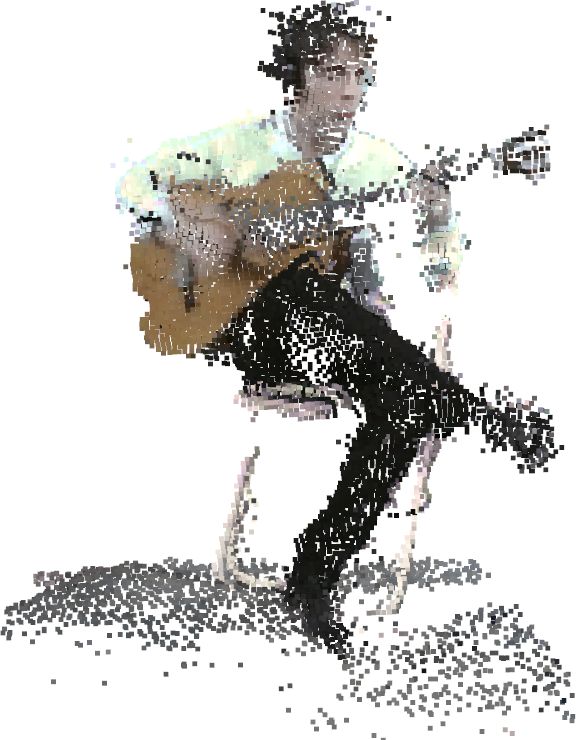
3D video
                       Vision Network                                                            Audio Network

                      Sparse Resnet18                                                                                 Mixture
                                                                       audio spectral features                      Spectrogram      Mixture

                                        Max Pooling
                                                      visual feature                                                                 Waveform
                                                                                                      U-Net
    ...

                       ...
                      Sparse Resnet18

                       learnable parameters
                                                              Fusion module
                                                                                                                           iSTFT

                                                                                                   Predicted Mask

FIG. 1. Overview diagram, showing the different parts of the model. Green area represents the vision network which extracts
a visual feature after analyzing each 3D video frames using a sparse Resnet18 architecture. Blue area represents the audio
network which extracts audio spectral features after analyzing the audio mixture spectrogram using a U-Net architecture. The
fusion module combines the multimodal extracted features to perform source separation.

1. Sparse 3D convolution                                                        through the network. To learn at different scales, the
                                                                                feature space is halved after two residual blocks and the
     The crucial operation within the vision network is
                                                                                receptive field is doubled by using a stride of 2. In addi-
the sparse 3D convolution. Considering predefined input
                                                                                tion, the depth of the filter size is doubled. Through the
coordinates Cin and output coordinates Cout , convolution
                                                                                network, ReLU is used as activation function and batch
on a 3D sparse tensor can be defined as:
                                                                                normalization is applied after sparse convolutions. At the
                  X                                                             top of the network we add a 3x3x3 sparse convolution
 T0 [x, y, z] =           W[i, j, k]T[x+i, y+j, z+k] (3)                        with K output channels and apply a max-pooling opera-
               i,j,k∈N (x,y,z)
                                                                                tion to adequate the dimensions of the extracted features.
                                                                                Figure 2 shows a schematic diagram of the Resnet18 ar-
for (x, y, z) ∈ Cout . Where N (x, y, z) = {(i, j, k)||i| ≤
                                                                                chitecture with sparse 3D convolutions.
L, |j| ≤ L, |k| ≤ L, (i + x, j + y, k + z) ∈ Cin }. W are
                                                                                    Finally, another max-pooling operation with sigmoid
the weights of the 3D kernel and 2L + 1 is the convo-
                                                                                activation is applied to all frame features which results
lution kernel size. Sparse 3D convolutions provide the
                                                                                in an extracted visual feature vector v ∈ [0, 1]1×K (See
necessary flexibility to efficiently learn from non-dense
                                                                                Fig. 1).
representations of variable size such as point clouds. Un-
like images or 2D videos where the information is densely
represented in a grid, point clouds contain lots of empty                       C. Audio Network
space. For this reason, it is inefficient to operate on them
                                                                                     We use a U-Net architecture with dense convolutions
using traditional convolutions.
                                                                                to extract spectral features from the audio mixture spec-
                                                                                trogram. U-Net was first introduced for biomedical im-
2. Vision architecture                                                          age segmentation22 and since then it has been adapted
    We use a Resnet18 neural network20 with sparse 3D                           for audio source separation in many cases8,10,23 . The
convolutions17 to extract features from each frame of a                         U-Net encoder-decoder structure learns multi-resolution
3D video. Resnet18 architecture was first introduced for                        features from the magnitude spectrogram. The encoder
the task of image recognition20 and since then it has                           halves the size of the feature maps by using a stride of 2
been successfully used in several computer vision tasks21 .                     and doubles the filter size while the decoder then reverses
Key to the Resnet18 architecture are the skip connec-                           this procedure by upsampling the size of the feature maps
tions within its residual blocks which assist convergence                       and halving the filter size. Similarly to Resnet18, skip
with negligible computational cost. The skip connection                         connections are also present in U-Net which allows low-
at the beginning of a residual block is then added at                           level information to be propagated through the network.
the end which helps to propagate low-level information                          The U-Net feature maps computed by the encoder are

J. Acoust. Soc. Am. / 4 February 2021                                                                                  Music source separation   3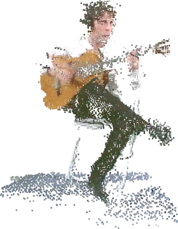
E. Learning Objective

           Max Pooling
                                                                              During the training of the network, the parameters
                                                                         of the model are optimized to reduce the binary cross
       3x3x3 SparseConv (K)                                              entropy (BCE) loss between each value of the predicted
                                                                         frequency mask M0 and the ideal binary mask MIBM .
          Block (512, x2)                                                Considering a mixture created by N sources, we first de-
                                                                         fine the ideal binary mask MIBM of the i-source as:
          Block (256, x2)
                                                                                          (
                                                                                           1 |Si (t, f )| ≥ |Sn (t, f )|∀n ∈ {1, . . . , N }
          Block (128, x2)                                                MIBM (t, f ) =
                                                    ReLU                                   0 otherwise,
           Block (64, x2)                                                                                                                (5)
                                                        +                where Si (t, f ) = STFT(si (t)). Then the loss function
          Average Pooling                                                takes the form:
                                             Batch Normalization
              ReLU                           3x3x3 SparseConv
                                                                                              L = BCE(M0 , MIBM )                       (6)
                                                    ReLU
         Batch Normalization
                                             Batch Normalization
                                                                         F. Dataset
       5x5x5 SparseConv (64)                 3x3x3 SparseConv
                                                                              While there are lots of audio datasets, there is data
                                                                         scarcity of 3D videos of performing musicians. For the
                                                                         purposes of this work, we capture 3D videos of twelve
               (a)                                      (b)              performers playing different instruments: cello, double
                                                                         bass, guitar, saxophone, and violin. In addition, we sep-
FIG. 2. (a) Schematic diagram of the sparse Resnet18 archi-              arately collect audio recordings of these instruments from
tecture used to extract features for each 3D video frames. (b)           existing audio datasets8,25 . Lastly, once all 3D video and
Schematic diagram of the sparse Resnet18 residual block.                 audio data was collected, we randomly associate audio
                                                                         and 3D video for each instrument. This will enable the
                                                                         model to learn and perform source separation with un-
                                                                         synchronized 3D video and audio.
accessed by the decoder at the same level of hierarchy
                                                                              3D video: We capture a dataset consisting on 3D
via concatenation. In this work, 7 layers for both the
                                                                         videos from several musicians playing different instru-
encoder and the decoder are used. Finally, the output of
                                                                         ments: cello, doublebass, guitar, saxophone, and violin.
the decoder is spectral features S ∈ R256×256×K with the
                                                                         Recordings were conducted using a single Azure Kinect
same size as the input spectrogram and K channels.
                                                                         DK placed one meter above the floor and capturing a
                                                                         frontal view of the musician at a distance of two meters.
D. Fusion module                                                         Azure Kinect DK comprises a depth camera and a color
                                                                         camera. The depth camera was capturing a 75◦ ×65◦ field
    Considering the visual feature from the vision net-                  of view with a 640 × 576 resolution while the color cam-
work v ∈ [0, 1]1×K and the spectral features from the                    era was capturing with a 1920 × 1080 resolution. Both
audio network S ∈ R256×256×K , the predicted spectro-                    cameras were recording at 15 fps and Open3D library
gram mask M0 ∈ [0, 1]256×256 is computed as:                             was then used to align depth and color streams and gen-
                                                                         erate a point cloud for each frame. The full 3D video
                                K
                               X                                       recordings span 1 hour of duration with an average of 12
                  M0 = σ             αk vk Sk + β                  (4)   different performers for each instrument.
                                                                              We increase our 3D video dataset collecting 3D
                               k=1
                                                                         videos from small ensemble 3D-video database 26 and
                                                                         Panoptic Studio 27 . In small ensemble 3D-video database,
where α ∈ R1×K and β ∈ R are learnable parameters. σ                     recordings are carried using three RGB-Depth Kinect v2
corresponds to the sigmoid activation function.                          sensors. LiveScan3D28 and OpenCV libraries are then
    In this work, the multimodal fusion is performed at                  used to align and generate point clouds for each frame
the end of the model as a linear combination like in                     given each camera point of view and sensor data. The
PixelPlayer8 . Other fusion techniques exist to condition                average video recordings is 5 minutes per instrument and
an audio network using visual features12 . In early exper-               a single performer per instrument. In Panoptic Stu-
iments, we inserted visual features in the middle of the                 dio, recordings are carried out using ten Kinect sensors.
audio network and in all decoder layers using a feature-                 In this case, recordings span two instrument categories:
wise linear modulation approach24 . However, model con-                  cello and guitar. The average video recordings is 2 min-
vergence turned out to be slower with no increase in per-                utes per instrument and a single performer per instru-
formance.                                                                ment.

4    J. Acoust. Soc. Am. / 4 February 2021                                                                          Music source separation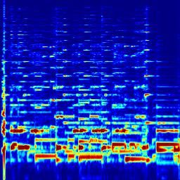
We use 75% of all 3D video recordings for training,
15% for validation, and the remaining 10% for testing.
Note that the training, validation and testing sets are
completely independent as there are no overlapping iden-
tities between them.
Audio: We collect audio recordings from Solos 25
and Music 8 datasets to create an audio dataset that com-
prises audio sources from the aforementioned five differ-
ent instruments. Both Solos and Music datasets gather
audio from Youtube which provides recordings in a va-
riety of acoustic conditions. In total, audio recordings
span 30 hours of duration with an average amount of
72 recordings per instrument and a mean duration of 5 (a)
minutes per recording.
We use 75% of all audio recordings for training, 15%
for validation, and the remaining 10% for testing.
G. Data preprocessing and data augmentation
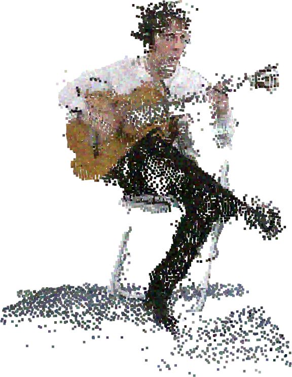
1. 3D videos
The following preprocessing procedure is applied to
all 3D videos. First, each frame, which consists of a mu-
sician point cloud, is scaled to fit within the cube [−1, 1]3
and centered in the origin. Then, the axes representing
the point clouds are set to have the same meaning for all (b) (c)
the collected 3D videos. This is: the body face direction
is z-axis, stature direction is y-axis, and the side direction
is x-axis (see Fig. 3).
During the training of the model, F point cloud
frames are randomly selected from each 3D video and a
combination of augmentation operations are performed
in both coordinates and color to increase the data diver-
sity. After augmentation, resulting frames are fed into
the vision network.
We randomly rotate, scale, shear and translate the
coordinates of the selected frames. We perform two ro-
tations. First rotation is on the y-axis with a random
angle ranging from −π to π and second rotation is on a
random axis with a random angle ranging from −π/6 to (d) (e)
π/6. Both axis and angles are sampled uniformly. The
scaling factor is also uniformly sampled and ranges from FIG. 3. Illustration of the coordinate augmentations applied
0.5 to 1.5 while the translation offset vector is sampled individually: (a) Original. (b) Random rotation. (c) Random
from a Normal distribution N1×3 (0, 0.42 ). Lastly, shear- scale. (d) Random shear. (e) Random translation. Red,
ing is applied along all axes and the shear elements are green, and blue arrows correspond to x,y,z-axis respectively.
sampled from N (0, 0.12 ). Figure 3 illustrates the differ-
ent augmentation operations applied to coordinates.
Regarding color, we distort the brightness and in-
tensity of the selected frames. Specifically, we alter color ditioning scenarios: when 3D videos consist only in a
value and color saturation with random amounts uni- sequence of depth point cloud frames, or when 3D videos
formly sampled ranging from -0.2 to 0.2 and -0.15 to 0.15 consist in a sequence of rgb-depth point cloud frames. In
respectively. We also apply color distortion to each point the case only depth information is available, we use the
via adding Gaussian noise on each rgb color channel. non-discretized coordinates as the feature vectors asso-
Gaussian noise is sampled from N (0, 0.052 ). Figure 4 ciated to each point. In the case rgb-depth information
illustrates the different augmentation operations applied is available, we use the rgb values as the feature vectors
to colors. associated to each point.
After data augmentation, each frame is represented
as a sparse tensor by discretizing the point cloud coor-
dinates using a voxel size of 0.02. Performance of the
model is further analyzed considering two different con-
J. Acoust. Soc. Am. / 4 February 2021 Music source separation 5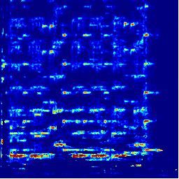
and the non-discretized coordinates are used as feature
                                                              vectors associated to each point.
                                                                   We train the whole model for 120k iterations using
                                                              stochastic gradient descent with a momentum 0.9. We
                                                              set K = 16 as the number of channels extracted by both
                                                              the vision and the audio network and we use a batch size
                                                              of 40 samples. Learning rate is set to 1 × 10⁻⁴ for the
                                                              vision network and to 1 × 10⁻³ for all the other learnable
                                                              parameters of the model. We select the weights with less
                                                              validation loss after the training process. Both training
                                                              and testing are conducted on a single Titan RTX GPU.
                                                              We use the Minkowski Engine30 for the sparse tensor
                                                              operations within the vision network and PyTorch31 for
           (a)                               (b)              the other operations required.

                                                              B. Evaluation metrics

                                                                   We measure the audio separation performance of the
                                                              model using the metrics from the BSS eval toolbox32 . In
                                                              a first step, the toolbox decomposes the estimated signal
                                                              sˆi as follows:

                                                                          sˆi = starget + einterf + enoise + eartif        (7)

                                                              Where starget = f (si ) is a version of the reference signal si
                                                              modified by an allowed distortion f . einterf stands for the
                                                              interference coming from unwanted sources found in the
                                                              original mixture, enoise denotes the sensor noise, and eartif
           (c)                               (d)
                                                              refers to the burbling artifacts which are self-generated by
                                                              the separation algorithm. Then, the objective metrics are
FIG. 4. Illustration of the color augmentations applied in-   computed as energy ratios in decibels (dB), where higher
dividually: (a) Original. (b) Random value. (c) Random        values are considered to be better. Source to distortion
saturation. (d) Gaussian noise.                               ratio (SDR) is defined as:

                                                                                                  kstarget k2
                                                                       SDR = 10 log10                                      (8)
2. Audio                                                                                 keinterf + enoise + eartif k2
     Audio recordings are converted to mono and resam-
                                                              Source to interference ratio (SIR) is defined as:
pled to 11025 Hz. During the training of the model, 6
seconds long snippets are randomly selected from each
audio recording. Short-time Fourier transform is then                                            kstarget k2
                                                                               SIR = 10 log10                              (9)
applied using a Hann window with size 1022 and a hop                                             keinterf k2
size of 256. The magnitude of the time-frequency repre-
sentation is selected and a log-frequency scale is applied.   Source to artifacts ratio (SAR) is defined as:
This results in a time frequency representation of size
256 × 256. As augmentation, audio snippets are scaled                                 kstarget + einterf + enoise k2
with respect to the amplitude by a random factor uni-              SAR = 10 log10                                         (10)
                                                                                                keartif k2
formly sampled ranging from 0.5 to 1.5.
                                                                   We also assess the separation performance using the
III. RESULTS                                                  scale-invariant source to distortion ratio33 (SI-SDR). SI-
                                                              SDR does not modify the reference signal si and evalu-
A. Implementation details                                     ates the separation performance within an arbitrary scale
                                                              factor. SI-SDR between a signal si and its estimated ŝi
    Initially, we pretrain the vision network on the 3D
                                                              is defined as:
object classification task modelnet4029 to assist the fu-
ture learning process. As modelnet40 data consist on
                                                                                                  kαsi k2

CAD models, point clouds are sampled from mesh sur-                       SI-SDR = 10 log10                        (11)
faces of the object shapes. For the pretraining, we also                                       kαsi − ŝi k2
discretize the coordinates setting the voxel size to 0.02
                                                              where α = argminα kαsi − ŝi k2 = ŝTi si /ksi k2 .

6    J. Acoust. Soc. Am. / 4 February 2021                                                              Music source separation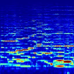
C. Baselines                                                       Conditioning the model using a single 3D depth
                                                              frame shows competitive performance compared with la-
    For comparison, we provide the separation perfor-         bel conditioning. This suggest the model is able to recog-
mance of the model when conditioned on instrument la-         nize the musical instrument from the 3D depth frame as
bels. To this end, we change the visual feature vector        in the case where the instrument label is explicitly given
v ∈ [0, 1]1×K for a one-hot vector h ∈ [0, 1]1×5 indicating   as a one-hot vector.
the instrument we aim to separate. We set the number
of spectral features extracted by the audio network ac-
cordingly, i.e. K = 5. We further refer to this as label      E. Varying number of sources
conditioning. Note that when using label conditioning,             We evaluate the source separation performance with
the one-hot vector will select one of the spectral features
                                                              regard to the number of sources present in the mix. Con-
extracted by the audio network (see Eq. 4). Thus, label
                                                              sidering best results from previous section, we fix F = 1
conditioning forces each spectral feature to correspond
                                                              as the number of frames provided to the vision net-
to a predicted spectrogram mask for each instrument.
                                                              work and asses the separation performance considering
For that reason, label conditioning can be interpreted as
                                                              N = 2, 3, 4 sources in the mix. In this case, performance
assessing the modeling capabilities of the audio network
                                                              is evaluated considering two types of 3D videos: when
alone for the separation task.
                                                              3D videos consist only in a sequence of depth frames,
    We also provide the upper bound separation perfor-
                                                              and when 3D videos consist in a sequence of rgb-depth
mance when signals are estimated using the ideal binary
                                                              frames. In the case only depth information is available,
masks (IBM).
                                                              we use the non-discretized coordinates as the feature vec-
                                                              tors associated to each point. In the case rgb-depth infor-
D. Varying number of frames                                   mation is available, we use the rgb values as the feature
                                                              vectors associated to each point.
    We are interested in evaluating the source separa-
tion performance depending on the number of 3D video
frames F used to condition the audio separation. We
fix N = 2 as the number of sources present in the mix         TABLE II. Source separation performance for different num-
and assess the separation performance when the vision         ber of sources (musical instruments) in the audio mixture.
network is provided with F = 1, 3, 5 frames. We take
consecutive frames with a distance of 1 second between
                                                              # Sources     Method      SDR       SIR     SAR      SI-SDR
them. In this case, performance is evaluated consider-
ing 3D videos that consist only in a sequence of depth                        label     6.10     12.44     9.73      3.94
frames, i.e. without color information. We use the non-                      depth      5.34     11.06    10.10      3.15
discretized coordinates as the feature vectors associated         2
                                                                           rgb-depth    6.14     12.29     9.97      3.98
to each point.
                                                                              IBM       15.20    21.63    16.84      14.47
                                                                              label     1.35     8.10      5.64      -2.75
TABLE I. Source separation performance for different number
                                                                             depth      -0.06    6.63      5.17      -5.01
of frames.                                                        3
                                                                           rgb-depth    0.86     7.27      5.69      -3.39
                                                                              IBM       11.80    19.55    12.93      10.56
# Frames       Method     SDR       SIR    SAR     SI-SDR
                                                                              label     -1.76    4.21      3.72      -7.03
                label     6.10     12.44   9.73     3.94
                                                                             depth      -2.48    3.34      4.05      -8.26
    1          depth      5.34     11.06   10.10    3.15          4
                                                                           rgb-depth    -3.39    2.79      3.48      -9.78
    3          depth      2.84      7.72   9.35     0.27
                                                                              IBM       9.14     16.65    10.26      7.66
    5          depth      0.84      5.16   9.25     -2.49
                IBM       15.20    21.63   16.84    14.47

                                                                  Regarding 3D visual conditioning, results reported
     Results in Table I show an improved separation per-      in Table II show a better separation performance when
formance as the number of 3D frames provided to the           the model is conditioned using rgb-depth information for
vision network decreases. Best results are achieved when      N = 2, 3 sources in the mix. Interestingly, when N = 4
the separation is conditioned with a single 3D frame.         better separation is achieved using only depth informa-
This means that the vision network has difficulties to        tion.
learn from multiple frames and cannot extract meaning-            3D visual conditioning provides similar separation
ful motion information from consecutive frames. Similar       performance as label conditioning when N = 2 sources in
cases are found in 2D visual source separation studies        the mix. Specifically, 3D rgb-depth conditioning slightly
where single frame conditioning provides strong separa-       outperforms label conditioning. This is likely due to the
tion performance11,12 .                                       linear combination within the fusion module which pro-

J. Acoust. Soc. Am. / 4 February 2021                                                           Music source separation      7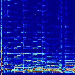
3D video        Mixture     Ground truth     Predicted     Ground truth     Predicted
                         frame        spectrogram      mask            mask        spectrogram     spectrogram

    Mixture pair
      (depth)

    Mixture pair
    (rgb-depth)

    FIG. 5. Visualization of the model separation performance using a single 3D video frame and two sources in the mix.

vides more expressivity to the model when combining            data are artificially associated and no synchronization be-
both vision and audio features.                                tween both modalities is provided. In addition, this can
     As we increase the number of sources in the mix,          be understood in relation to the literature where 2D sin-
i.e. N = 3, 4, label conditioning performs better than 3D      gle frame conditioning11,12 already achieves competitive
visual conditioning and its difference in performance in-      results given the difficulties of learning temporal infor-
creases with the number of sources. This shows that as         mation from multiple frames when no motion informa-
more sources are present in the mix, it becomes more           tion is given. However, higher performance is expected
difficult for the network to jointly learn from 3D repre-      by exploiting motion information as other 2D audio-
sentations and the audio information in order to perform       visual models do in audio-visual data synchronization
source separation. Figure 5 depicts qualitative results of     scenarios13,14 . Moreover, adopting a curriculum learning
the proposed model when two sources are present in the         strategy34 may be beneficial to improve the model sepa-
mix.                                                           ration performance when the number of sources present
                                                               in the mix increases12,13 . Regarding the type of 3D in-
                                                               formation used to condition the separation, rgb-depth
IV. DISCUSSION
                                                               appears to perform better overall although only depth is
     The work presented here indicates the effectiveness       better in the case when four sources are present in the
of a proposed learning model to perform music source           mix.
separation conditioned on 3D visual information. Specif-            The presented approach investigates to what extent
ically, 3D visual conditioning achieves competitive audio      point clouds can be used for guiding source separation,
separation performance compared to label conditioning.         thus enabling potential applicability in the VR/AR do-
     Best separation performance is achieved when con-         main. VR/AR systems benefit from knowing the sound
ditioning the model using a single 3D frame. This makes        and the location of each source in a 3D environment
sense in the current scenario where 3D video and audio         to simulate basic acoustic phenomena such as interau-

8    J. Acoust. Soc. Am. / 4 February 2021                                                            Music source separation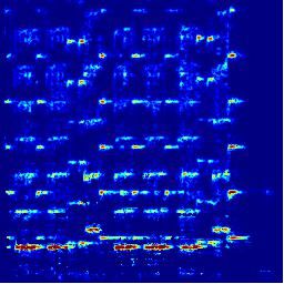
ral time differences and interaural level differences. 3D               8 H. Zhao, C. Gan, A. Rouditchenko, C. Vondrick, J. McDermott,
visual acquisition systems allow to capture the 3D envi-                  and A. Torralba, “The sound of pixels,” in Proceedings of the
                                                                          European conference on computer vision (ECCV) (2018), pp.
ronment, but the recorded sound sources are usually far                   570–586.
from the acoustic sensor and therefore sound needs to be                9 X. Xu, B. Dai, and D. Lin, “Recursive visual sound separation
separated and associated to each source for further au-                   using minus-plus net,” in Proceedings of the IEEE International
ralization. By learning jointly from 3D point clouds and                  Conference on Computer Vision (2019), pp. 882–891.
audio, the proposed model is able to separate the sounds,              10 R. Gao and K. Grauman, “Co-separating sounds of visual ob-

given the sources of interest are represented as 3D point                 jects,” in Proceedings of the IEEE International Conference on
                                                                          Computer Vision (2019), pp. 3879–3888.
clouds. This opens a new research direction which can                  11 L. Zhu and E. Rahtu, “Separating sounds from a single image,”
contribute to better simulation of acoustic phenomena in                  arXiv preprint arXiv:2007.07984 (2020).
VR/AR applications.                                                    12 O. Slizovskaia, G. Haro, and E. Gómez, “Conditioned source
                                                                          separation for music instrument performances,” arXiv preprint
                                                                          arXiv:2004.03873 (2020).
V. CONCLUSIONS                                                         13 H. Zhao, C. Gan, W.-C. Ma, and A. Torralba, “The sound of

     In this paper, a deep learning model for music source                motions,” in Proceedings of the IEEE International Conference
                                                                          on Computer Vision (2019), pp. 1735–1744.
separation conditioned on 3D point clouds has been pro-                14 C. Gan, D. Huang, H. Zhao, J. B. Tenenbaum, and A. Torralba,
posed. The model jointly learns from 3D visual informa-                   “Music gesture for visual sound separation,” in Proceedings of
tion and audio in a self-supervised fashion. Results show                 the IEEE/CVF Conference on Computer Vision and Pattern
the effectiveness of the model when conditioned using a                   Recognition (2020), pp. 10478–10487.
single frame and for a modest number of sources present                15 M.  Vorländer, “Auralization,” Aachen.: Springer (2008).
in the audio mixture. 3D visual conditioning, as opposed               16 Y. Wang, A. Narayanan, and D. Wang, “On training targets for
to 2D, enables potential applicability in virtual and aug-                supervised speech separation,” IEEE/ACM transactions on au-
                                                                          dio, speech, and language processing 22(12), 1849–1858 (2014).
mented reality applications where information about the                17 B. Graham, “Sparse 3d convolutional neural networks,” in Pro-
sound and the location of each source in the 3D environ-                  ceedings of the British Machine Vision Conference (BMVC),
ment is required for further auralization. As future work,                BMVA Press (2015), pp. 150.1–150.9.
exploiting also spatial audio cues caused by the location              18 E.  Fonseca, J. Pons Puig, X. Favory, F. Font Corbera, D. Bog-
of sound sources in the 3D environment may help to sep-                   danov, A. Ferraro, S. Oramas, A. Porter, and X. Serra,
arate same instrument sources. In addition, multimodal                    “Freesound datasets: a platform for the creation of open au-
                                                                          dio datasets,” in Hu X, Cunningham SJ, Turnbull D, Duan Z,
models that jointly learn from audio and point clouds                     editors. Proceedings of the 18th ISMIR Conference; 2017 oct 23-
could improve auditory 3D scene understanding.                            27; Suzhou, China.[Canada]: International Society for Music
                                                                          Information Retrieval; 2017. p. 486-93., International Society
                                                                          for Music Information Retrieval (ISMIR) (2017).
ACKNOWLEDGMENTS                                                        19 See supplementary material at github.com/francesclluis/
                                                                          point-cloud-source-separation.
    This project has received funding from the Euro-                   20 K. He, X. Zhang, S. Ren, and J. Sun, “Deep residual learning
pean Union’s Horizon 2020 research and innovation pro-                    for image recognition,” in Proceedings of the IEEE conference on
gramme under the Marie Sklodowska-Curie grant agree-                      computer vision and pattern recognition (2016), pp. 770–778.
ment No 812719. The authors thank A. Mayer for tech-                   21 A. Khan, A. Sohail, U. Zahoora, and A. S. Qureshi, “A survey of

nical support.                                                            the recent architectures of deep convolutional neural networks,”
                                                                          Artificial Intelligence Review 53(8), 5455–5516 (2020).
                                                                       22 O. Ronneberger, P. Fischer, and T. Brox, “U-net: Convolutional
1 E. Cano, D. FitzGerald, A. Liutkus, M. D. Plumbley, and F.-             networks for biomedical image segmentation,” in International
  R. Stöter, “Musical source separation: An introduction,” IEEE          Conference on Medical image computing and computer-assisted
  Signal Processing Magazine 36(1), 31–40 (2018).                         intervention, Springer (2015), pp. 234–241.
2 A. Défossez, N. Usunier, L. Bottou, and F. Bach, “Music             23 A. Jansson, E. Humphrey, N. Montecchio, R. Bittner, A. Ku-

  source separation in the waveform domain,” arXiv preprint               mar, and T. Weyde, “Singing voice separation with deep u-net
  arXiv:1911.13254 (2019).                                                convolutional networks,” in 18th International Society for Music
3 F.-R. Stöter, S. Uhlich, A. Liutkus, and Y. Mitsufuji, “Open-          Information Retrieval Conference (2017), pp. 23–27.
                                                                       24 E. Perez, F. Strub, H. De Vries, V. Dumoulin, and A. Courville,
  unmix - a reference implementation for music source separation,”
  Journal of Open Source Software 4(41), 1667 (2019).                     “Film: Visual reasoning with a general conditioning layer,” in
4 D.                                                                      Proceedings of the AAAI Conference on Artificial Intelligence
      Samuel, A. Ganeshan, and J. Naradowsky, “Meta-learning              (2018), Vol. 32.
  extractors for music source separation,” in ICASSP 2020-2020
                                                                       25 J. F. Montesinos, O. Slizovskaia, and G. Haro, “Solos: A dataset
  IEEE International Conference on Acoustics, Speech and Signal
  Processing (ICASSP), IEEE (2020), pp. 816–820.                          for audio-visual music analysis,” in 2020 IEEE 22nd Inter-
5 F. Lluı́s, J. Pons, and X. Serra, “End-to-end music source separa-      national Workshop on Multimedia Signal Processing (MMSP),
                                                                          IEEE (2020), pp. 1–6.
  tion: Is it possible in the waveform domain?,” Proc. Interspeech
                                                                       26 D. Thery and B. Katz, “Anechoic audio and 3d-video content
  2019 4619–4623 (2019).
6 H. Zhu, M. Luo, R. Wang, A. Zheng, and R. He, “Deep audio-              database of small ensemble performances for virtual concerts,”
                                                                          in 23rd International Congress on Acoustics, German Acoustical
  visual learning: A survey,” arXiv preprint arXiv:2001.04758             Society (DEGA) (2019), pp. 739–46.
  (2020).
                                                                       27 H. Joo, T. Simon, X. Li, H. Liu, L. Tan, L. Gui, S. Banerjee,
7 R. Gao, R. Feris, and K. Grauman, “Learning to separate ob-
                                                                          T. Godisart, B. Nabbe, I. Matthews, et al., “Panoptic studio: A
  ject sounds by watching unlabeled video,” in Proceedings of the         massively multiview system for social interaction capture,” IEEE
  European Conference on Computer Vision (ECCV) (2018), pp.               transactions on pattern analysis and machine intelligence 41(1),
  35–53.

J. Acoust. Soc. Am. / 4 February 2021                                                                        Music source separation    9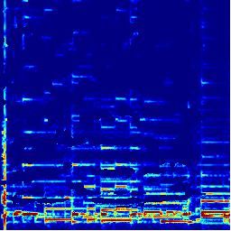
190–204 (2017).                                                     31 A.Paszke, S. Gross, F. Massa, A. Lerer, J. Bradbury, G. Chanan,
28 M.  Kowalski, J. Naruniec, and M. Daniluk, “Livescan3d: A fast        T. Killeen, Z. Lin, N. Gimelshein, L. Antiga, et al., “Pytorch:
   and inexpensive 3d data acquisition system for multiple kinect v2     An imperative style, high-performance deep learning library,” in
   sensors,” in 2015 international conference on 3D vision, IEEE         Advances in neural information processing systems (2019), pp.
   (2015), pp. 318–325.                                                  8026–8037.
                                                                       32 E. Vincent, R. Gribonval, and C. Févotte, “Performance mea-
29 Z. Wu, S. Song, A. Khosla, F. Yu, L. Zhang, X. Tang, and J. Xiao,
   “3d shapenets: A deep representation for volumetric shapes,”           surement in blind audio source separation,” IEEE transactions on
   in Proceedings of the IEEE conference on computer vision and           audio, speech, and language processing 14(4), 1462–1469 (2006).
   pattern recognition (2015), pp. 1912–1920.                          33 J. Le Roux, S. Wisdom, H. Erdogan, and J. R. Hershey, “Sdr–
30 C.Choy, J. Gwak, and S. Savarese, “4d spatio-temporal convnets:        half-baked or well done?,” in ICASSP 2019-2019 IEEE Inter-
  Minkowski convolutional neural networks,” in Proceedings of the         national Conference on Acoustics, Speech and Signal Processing
  IEEE Conference on Computer Vision and Pattern Recognition              (ICASSP), IEEE (2019), pp. 626–630.
  (2019), pp. 3075–3084.                                               34 Y. Bengio, J. Louradour, R. Collobert, and J. Weston, “Curricu-
                                                                          lum learning,” in Proceedings of the 26th annual international
                                                                          conference on machine learning (2009), pp. 41–48.

10      J. Acoust. Soc. Am. / 4 February 2021                                                                     Music source separation
You can also read