Just Pick a Sign: Optimizing Deep Multitask Models with Gradient Sign Dropout - NeurIPS
←
→
Page content transcription
If your browser does not render page correctly, please read the page content below
Just Pick a Sign: Optimizing Deep Multitask Models
              with Gradient Sign Dropout

          Zhao Chen                      Jiquan Ngiam                      Yanping Huang
         Waymo LLC                      Google Research                   Google Research
    Mountain View, CA 94043          Mountain View, CA 94043           Mountain View, CA 94043
      zhaoch@waymo.com                jngiam@google.com                 huangyp@google.com

         Thang Luong                   Henrik Kretzschmar                   Yuning Chai
        Google Research                    Waymo LLC                        Waymo LLC
    Mountain View, CA 94043          Mountain View, CA 94043           Mountain View, CA 94043
    thangluong@google.com            kretzschmar@waymo.com               chaiy@waymo.com

                                       Dragomir Anguelov
                                          Waymo LLC
                                     Mountain View, CA 94043
                                      dragomir@waymo.com

                                             Abstract
         The vast majority of deep models use multiple gradient signals, typically corre-
         sponding to a sum of multiple loss terms, to update a shared set of trainable weights.
         However, these multiple updates can impede optimal training by pulling the model
         in conflicting directions. We present Gradient Sign Dropout (GradDrop), a proba-
         bilistic masking procedure which samples gradients at an activation layer based on
         their level of consistency. GradDrop is implemented as a simple deep layer that can
         be used in any deep net and synergizes with other gradient balancing approaches.
         We show that GradDrop outperforms the state-of-the-art multiloss methods within
         traditional multitask and transfer learning settings, and we discuss how GradDrop
         reveals links between optimal multiloss training and gradient stochasticity.

1   Introduction
Deep neural networks have fueled many recent advances in the state-of-the-art for high-dimensional
nonlinear problems. However, when distilled down to its most basic elements, deep learning relies
on the humble gradient as the optimization signal which drives its complex algorithmic machinery.
Indeed, the desire to properly leverage gradients has spurred a wealth of research into optimization
strategies which has led to faster, more stable model training [36].
However, the literature has habitually glossed over an increasingly crucial detail: most gradient
signals are sums of many smaller gradient signals, often corresponding to multiple losses. A broad
array of models fall under this category, including ones not traditionally considered multitask; for
example, multiclass classifiers can be split into a loss per class, and object detectors conventionally
break down their predictions along various bounding box dimensions. It is uncertain, and in fact
unlikely, that a naïve sum of these individual signals would produce the best solution.
Deep learning theory tells us that the local minima found in single-task models through simple
gradient updates are generally of high quality [4]. However, such a claim should be reevaluated in
the context of multitask loss surfaces, where minima of each constituent loss may exist at different

34th Conference on Neural Information Processing Systems (NeurIPS 2020), Vancouver, Canada.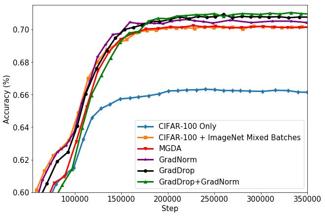
network weight settings, which results in many poor minima of the sum loss. Such undesirable
minima are avoided if we encourage the network to seek out critical points that are joint minima – i.e.
critical points that lie near a local minimum of all the constituent loss functions.
To generally address such issues, deep multitask learning studies properties of models with multiple
outputs and has given birth to methods to balance relative gradient magnitudes [3; 17] or tune the full
gradient tensor [38]. Still, methods that explicitly tackle joint loss optimization are rare. Works such
as [37; 47] do so by finding a common gradient descent direction for all losses, but such methods
operate by removing suboptimal gradient components. Such reductive processes are still susceptible
to local minima and discourage inter-task competition – competition which evidence suggests can
be beneficial [6; 46]. Our proposed method not only provides theoretical guarantees of joint loss
minima but also allows gradients to compete, and thus avoids the same pitfalls as reductive gradient
algorithms. To the best of our knowledge our method is the first with this set of desirable properties.
We motivate our method, Gradient Sign Dropout (GradDrop), by noting that when multiple gradient
values try to update the same scalar within a deep network, conflicts arise through differences in sign
between the gradient values. Following these gradients blindly leads to gradient tug-of-wars and to
critical points where constituent gradients can still be large (and thus some tasks perform poorly).
To alleviate this issue, we demand that all gradient updates are pure in sign at every update position.
Given a list of (possibly) conflicting gradient values, we algorithmically select one sign (positive or
negative) based on the distribution of gradient values, and mask out all gradient values of the opposite
sign. A basic schematic of the method is presented in Figure 1.

Figure 1: GradDrop schematic for two losses and one scalar. In both cases, we calculate P (from
Equation 1), which tells us the probability of keeping rs with positive signs. On the left, P =
0.5 ⇤ (1 + (3 + 1)/(|3| + |1|)) = 1.0, so we keep positive rs with 100% probability. On the right,
P = 0.5 ⇤ (1 + (7 3)/(|7| + | 3|)) = 0.7, so we keep positive rs with 70% probability.

The motivation behind GradDrop parallels the well-known relationship between gradient stochasticity
and model robustness [18; 39; 40]. When a network finds a narrow, low-quality minimum, the
inherent noise within the batched gradient updates serves to kick the model into broader, more
robust minima. Similarly, GradDrop assigns a quality score to each gradient update based on its sign
consistency, and adds stochasticity along axes where gradients tend to conflict more. An important
consequence of this logic is that GradDrop continues triggering until the model finds a minimum that
is a joint minimum for all losses (see Section 4.1 for proof).
Our primary contributions are as follows:

      1. We present Gradient Sign Dropout (GradDrop), a modular layer that works in any network
         with multiple gradient signals and incurs no additional compute at inference.
      2. We show theoretically and in simulation that GradDrop leads to more stable convergence
         points than naïve gradient descent algorithms.
      3. We demonstrate the efficacy of GradDrop on multitask learning, transfer learning, and
         complex single-task models like 3D object detectors for a variety of network architectures.

                                                   2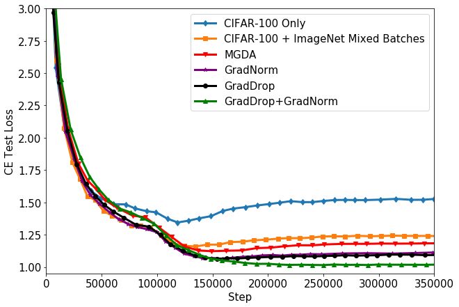
2     Related Work
Optimization via gradient descent is one of the key pillars of deep learning. Apart from the
traditional optimization methods [8; 19; 32; 33; 49], there has been a research thrust on developing
different ways to apply gradients to deep networks [2; 7; 10; 15; 36; 45; 50]. The success of such
methods comes in part because optimization in single-task models generally converges to high-quality
minima [4]. Also important is the relationship between stochasticity and model robustness; as with
GradDrop, noisy gradients help repel poor local minima in favor of wider, more robust critical points
[18; 39; 40]. These insights are crucial and worth revisiting for multitask environments.
Multitask learning presents a challenging problem for optimization, as the loss surface now consists
of many smaller loss surfaces. As a subject of study, multitask learning predates deep learning [1; 6],
but its power in helping model generalization and transferring information between correlated tasks
[30; 48] make it especially relevant in the deep learning era. Although a large part of multitask
research focuses on developing new network architectures [16; 20; 23; 25; 28; 29; 31] or new loss
functions [17], we focus on methods that explicitly interact with the gradients, which tend to be more
lightweight and modular. GradNorm [3] modifies gradient magnitudes to ensure that tasks train at
approximately the same rate. MGDA, the Multiple Gradient Descent Algorithm [6; 37], finds a linear
combination of gradients that reduces every loss function simultaneously. PCGrad [47] projects
conflicting gradients to each other, which achieves a similar simultaneous descent effect as MGDA.
Many other applications which are not traditionally considered multitask can benefit from this
work. Vision applications such as object detection [24; 34; 35; 51] and instance segmentation [11]
explicitly construct multiple losses to arrive at one consolidated result. Language models that employ
seq2seq predictions [44] make multiple predictions and create multiple gradient conflicts when
backpropagating through time. Domain adaptation and transfer learning [9; 12; 43], topics in which
many powerful specialized techniques have been developed, still often rely on multiple losses and
thus can benefit from general multitask approaches. Our approach here, although wrapped in the
language of multitask learning, has a much wider range of applicability on deep models in general.

3     Gradient Dropout
3.1   Basic Concepts

Gradient Sign Dropout is applied as a layer in any standard network forward pass, usually on the
final layer before the prediction head to save on compute overhead and maximize benefits during
backpropagation. In this section, we develop the GradDrop formalism. Throughout, denotes
elementwise multiplication after any necessary tiling operations (if any) are completed.
To implement GradDrop, we first define the Gradient Positive Sign Purity, P, as
                                          ✓      P          ◆
                                        1             rLi
                                  P=        1+ P    i
                                                              .                                       (1)
                                        2          i |rLi |

P is bounded by [0, 1]. For multiple gradient values ra Li at some scalar a, we see that P = 0 if
ra Li < 0 8i, while P = 1 if ra Li > 0 8i. Thus, P is a measure of how many positive gradients
are present at any given value. We then form a mask for each gradient Mi as follows:
                 Mi = I[f (P) > U ] I[rLi > 0] + I[f (P) < U ] I[rLi < 0]                             (2)
for I the standard indicator function and f some monotonically increasing function (often just the
identity) that maps [0, 1] 7! [0, 1] and is odd around (0.5, 0.5). U is aP
                                                                         tensor composed of i.i.d U (0, 1)
random variables. The Mi is then used to produce a final gradient Mi rLi .
A simple example of a GradDrop step is given in Figure 1 for the trivial activation f (x) = x.

3.2   Extension to Transfer Learning and other Batch-Separated Gradient Signals

A complication arises when different gradients correspond to different examples, e.g. in mixed-batch
transfer learning where transfer and source examples connect to separate losses. The different gradi-
ents at an activation layer would then not interact, which makes GradDrop the trivial transformation.

                                                    3
We also cannot just blindly add gradients along the batch dimension, as the information present in
each gradient is conditional on that gradient’s particular inputs. Generally, deep nets consolidate
information across a batch by summing gradient contributions at a trainable weight layer. To correctly
extend GradDrop to batch-separated gradients, we will do the same.
For a given layer of activations A of shape (B, F ), we imagine there exists an additional weight layer
W (A) of shape (F ) composed of 1.0s, and consider the forward pass A 7! W (A) A. W (A) is a
virtual layer and is not actually allocated memory during training; we only use it to derive meaningful
mathematical properties. Namely, we can then calculate the gradient via the chain rule to arrive at
X
rW (A) Li = (A rA Li ) (3)
batch
where the final sum is taken over the batch dimension1 . In other words, premultiplying the gradient
values by the input allows us to meaningfully sum over the batch dimension to calculate P and the
Mi s. In practice, because we are only interested in rW (A) insofar as it changes the sign content of
rA , we will only premultiply by the sign of the input.
3.3 Full GradDrop Algorithm
The full GradDrop algorithm calculates the sign purity measure P at every gradient location, and
constructs a mask for each gradient signal across T tasks. We specify the details in Algorithm 1.
Algorithm 1 Gradient Sign Dropout Layer (GradDrop Layer)
1: choose monotonic activation function f . Usually just f (p) = p
2: choose input layer of activations A . Usually the last shared layer
3: choose leak parameters {`1 , . . . , `n } 2 [0, 1] . For pure GradDrop set all to 0
4: choose final loss functions L1 , . . . , Ln
5: function BACKWARD(A, L1 , . . . , Ln ) . returns total gradient after GradDrop layer
6: for i in {1, . . . , n} do
7: calculate Gi = sgn(A) rA Li . sgn(A) inspired by Equation 3
8: if Gi is batchP separated then
9: Gi ⇣
batchdim Gi ⌘
P
G
10: calculate P = 1
1+ Pi i . P has the same shape as G1
2 i |Gi |
11: sample U , a tensor with the same shape as P and U [i, j, . . .] ⇠ Uniform(0, 1)
12: for i in {1, . . . , n} do
13: calculate Mi = I[f (P) > U ] I[Gi > 0] + I[f (P) < U ] I[Gi < 0]
P
14: set newgrad = i (`i + (1 `i ) ⇤ Mi ) rA Li
15: return newgrad
For many of our experiments, we renormalize the final gradients so that ||r||2 remains constant
throughout the GradDrop process. Although not practically required, this ensures that GradDrop does
not alter the global learning rate and thus observed benefits result purely from GradDrop masking.
Note also the introduction of the leak parameters `i . Setting `i > 0 allows some original gradient to
leak through, which is useful when losses have different priorities – for example, in transfer learning,
we prioritize performance on the transfer set. For more details see Section 4.3.
3.4 GradDrop Theoretical Properties
We now present and prove the main theoretical properties for our proposed GradDrop algorithm.
Proposition 1 (GradDrop stable points are joint minima): Given loss functions L1 , . . . , Ln and
any collection of scalars W for which rw L1 , . . . , rw Ln are well-defined, the GradDrop update
(GD)
signal rw at any position w 2 W is always zero if and only if rw Li = 0, 8i.
1
The initialization of the virtual layer is not only meant to keep the forward logic trivial. It is relevant also in
the derivation of Equation 3, as it gives us that rA Li = W (A) rW (A) A Li = rW (A) A Li
4Proof: Consider n loss functions, indexed L1 , . . . , Ln , and their gradients
P rw Li for w 2 W. Clearly,
if rw Li = 0, 8i, then that w is trivially a critical point for the sum loss i Li . However, the converse
is also true under GradDrop updates. Namely, if there exists some j for which rw Lj 6= 0, without
loss of generality assume that rw Lj > 0. According to Equation 1, P > 0 at w. Thus f (P) > 0 (as
it is monotonically increasing), so there is a nonzero (f (P)) chance that we keep all positive signed
(GD)
gradients and thus a nonzero chance that rw rw Lj > 0. ⇤
Proposition 2 (GradDrop r norms sensitive to every loss): Given continuous component loss
functions Li (w) with local minima w(i) and a GradDrop update r(GD) , then to second order around
each w(i) , E[|r(GD) L|2 ] is monotonically increasing w.r.t. |w w(i) |, 8i.
Proof: Set := d 0 for | 0 | = 1. To second order, around a minimum value w(i) a loss function
has the form Li (w(i) + ) ⇡ Li (w(i) ) + 12 T H (Li ) (w(i) ) = Li (w(i) ) + 12 d2 T0 H (Li ) (w(i) ) 0 for
positive definite Hessian H (Li ) . Because T0 H (Li ) (w(i) ) 0 > 0, rLi at w(i) + is proportional to
d. As d increases, so will the magnitude of each rLi component, which then immediately increases
the total expected gradient magnitude induced by GradDrop. ⇤
From Proposition 1, we see that GradDrop will result in a zero gradient update only when the system
finds a perfect joint minimum between all component losses. Not only that, but Proposition 2 implies
that GradDrop induces proportionally larger gradient updates with distance from any component loss
function minimum, regardless of the value of the total loss. The error signals induced by GradDrop
are thus sensitive to every task, rather only relying on a sum signal. This sensitivity also increases
monotonically with distance from any close local minimum for any component task. Thus, GradDrop
optimization will seek out joint minima, but even when such minima do not strictly exist Proposition
2 shows GradDrop will seek out system states that are at least close to joint minima. For a clear
illustration of this effect in one dimension, please refer to Section 4.1.
A potential concern could be that by being sensitive to every loss function, GradDrop updates are too
noisy and the overall system trains more slowly. However, that is not the case, as GradDrop updates
on expectation are equivalent with standard SGD updates.
P
Proposition 3 (Statistical Properties): Suppose for 1D loss function L = i Li (w) an SGD
gradient update with learning rate changes total loss by the linear estimate L(SGD) = |rL|2
0. For GradDrop with activation function (see Eq. 2) f (p) = k(p 0.5) + 0.5 for k 2 [0, 1] (with
default setting is k = 1), we have:
1. For k = 1, L(SGD) = E[ L(GD) ]
2. E[ L(GD) ] 0 and has magnitude monotonically increasing with k.
3. Var[ L(GD) ] is monotonically decreasing with respect to k.
We present the proof of this proposition in the Appendix, along with generalizing it to arbitrary
activation functions. ⇤
Importantly, even though GradDrop has a stochastic element, it provides the same expected movement
in the total loss function as in vanilla SGD. Also important is the hyperparameter k, which controls
the tradeoff between how much the GradDrop update follows the overall gradient and how much noise
GradDrop induces for inconsistent gradients. A smaller value of k implies a larger penalty/noise scale,
and a value of k = 0 means we randomly choose a sign for every gradient value. We call the k = 0
case Random GradDrop and show it generally compares unfavorably to k > 0, but our evidence does
not preclude a situation where the higher noise in the k = 0 case may be desirable. Indeed, in most
of our experiments the k = 0 Random GradDrop setting still outperforms the baseline.
4 Experiments with GradDrop
In this section we present the main experimental results related to GradDrop. All experiments are run
on NVIDIA V100 GPU hardware. We will provide relevant hyperparameters within the main text,
but we relegate a complete listing of hyperparameters to the Appendix. We also rely exclusively on
standard public datasets, and thus move discussion of most dataset properties to the Appendices.
All multitask baselines (including PCGrad, to keep compute overhead tractable) and the GradDrop
layer are applied to the final layer before the prediction heads to keep compute overhead tractable. We
5primarily compare to other state-of-the-art multitask methods, which include GradNorm [3], MGDA
[37], and PCGrad [47]. Descriptions of all these methods were given in Section 2.
For completion, we also compare to Gradient Clipping (e.g. [50]) and Gradient Penalty [10]. Although
not strictly multitask methods, these gradient-based methods enjoy wide popularity and will provide
evidence that principled single-task methods are not enough to optimize a true multitask model.
4.1 A Simple One-Dimensional Example
(a) Sum of sinusoids loss function (b) Loss curves for one random run (c) Summary results for 200 runs
Figure 2: GradDrop toy example. (a) A synthetic 1D loss function composed of five sines. (b) Loss
curves for GradDrop and baselines given a random initialization of the trainable weight. (c) Boxplot
of final converged loss values when the methods in b. are run 200 times.
We illustrate GradDrop in one dimension. In Figure 2 we present results on a simple toy system, with
a loss function that is the sum of five sines of the form L(x; a, b) = sin(ax + b) + 1. The final loss is
shown in Figure 2(a). Note that although each Li has identical periodic local minima, the sum loss
has a wide distribution of local minima of variable quality.
We now initialize the one weight w to a random value and run various optimization techniques for
10000 steps. In Figure 2(b) we plot the loss curves for one example trial. We note that PCGrad [47]
does not train in this low-dimensional setting, as any sign conflict would result in PCGrad zeroing the
gradients. For fairness, we include a slight modification of PCGrad called iterative PCGrad which
still works in low dimensions (for details see Appendix). We also include Random GradDrop, which
is a weak version of GradDrop where f (P) is set to 0.5 everywhere. We see that GradDrop has the
best performance of all methods tested. Such a conclusion is further reinforced when we run this
experiment 200 times and plot the statistics of the final results, which are shown in Figure 2(c).
Multiple algorithms (GradDrop, Random GradDrop, and Iterative PCGrad) tend to find the deepest
minimum, but GradDrop still performs better. We attribute this to the success of our sign purity
measure P at properly emphasizing gradient directions with higher levels of consistency.
4.2 Multitask Learning on Celeb-A
We first test GradDrop on the multitask learning dataset CelebA [26], which provides 40 binary
attributes based on celebrity facial photos. CelebA allows us to test GradDrop in a truly archetypal
multitask setting.
We also use a standard shallow convolutional network to perform this task. Our network consists
only of common layers (Conv, Pool, Batchnorm, FC Layers) and contains 9 total layers along with
40 predictive heads. The results of our experiments are summarized in Figure 3 and Table 1.
We see that GradDrop outperforms all other methods. Although the improvements may seem mild in
Table 1, they are substantial for this dataset and Figure 3(a) reveals a visually significant effect. Figure
3(b) also shows an ablation study of performance when we choose to marginalize our gradient signal
across the batch dimension, as suggested by Section 3.2. Although our gradient signal for CelebA
is not batch-separated and thus we are not strictly required to sum the GradDrop signal across our
batches, this operation improves GradDrop’s memory and compute efficiency, and also can clearly
improve model performance. As there are thus few disadvantages from using the sum-over-batch
strategy, all further GradDrop runs in this paper will use sum-over-batch.
6(a) CelebA maximum F1 scores (b) GradDrop batch marginalization (c) Gradient consistency over time
Figure 3: Experiments with GradDrop on CelebA.
Table 1: Multitask Learning on CelebA. We repeat training runs and report standard deviations of
0.04% for F1 Score and 0.02% for accuracy.
Method Error Rate (%) # Max F1 Score " Speed Compared to Baseline "
Baseline 8.71 29.35 1.00
Gradient Clipping [50] 8.70 29.34 1.00
Gradient Penalty [10] 8.63 29.43 0.35
MGDA [37] 10.82 26.00 0.25
PCGrad [47] 8.72 29.25 0.20
GradNorm [3] 8.68 29.32 0.41
Random GradDrop 8.60 29.42 0.45
GradDrop (ours) 8.52 29.57 0.45
Furthermore, Figure 3(c) plots the percentage of gradients passed by the GradDrop layer, for both a
GradDrop model and a baseline model2 . This percentage correlates to the degree of sign consistency
of gradients at the GradDrop layer. This metric does not improve at all when training the baseline,
but improves appreciably when GradDrop is enabled, suggesting that the critical points found by
GradDrop have more consistent gradients and thus higher probability of being a joint minimum.
It is interesting to note that GradDrop also overfits less. We posit that GradDrop is a good regularizer
due to its tendency to reject weak loss minima that may overfit. The only stronger regularizer may be
GradNorm [3], but GradNorm explicitly curtails overfitting with its ↵ hyperparameter.
CelebA with its T = 40 tasks also presents us with an excellent opportunity to test method speed.
Looking at the last column of Table 1, we see that GradDrop is the fastest of the multitask methods
tried (not counting gradient clipping, which is a general single-task method), possibly because it only
requires a simple calculation at each tensor position of O(T ) rather than multiple iterative steps like
MGDA or O(T 2 ) orthogonal projections like PCGrad.
4.3 Transfer Learning on CIFAR-100
We now use GradDrop in a transfer learning setting, which is a batch-separated setting (see Section
3.2). We transfer ImageNet2012 [5] to CIFAR-100 [21] by using input batches consisting of half
CIFAR-100 and half ImageNet2012 examples. Each dataset has its own predictive head and loss.
We use a more complex network based on DenseNet-100 [13], both to increase performance and to
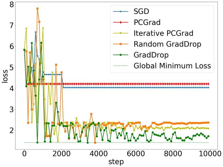
test GradDrop with more complex network topologies. Our results are shown in Table 2 and Figure 4,
where we present the best accuracy achieved by each method and the corresponding loss3 ; we include
the loss as it is generally smoother.
We see that the best model uses a combination of GradDrop and GradNorm [3], although the
GradDrop-Only model also performs well. As in the CelebA experiments presented in Section 4.2,
the performance gap is larger when the baseline models overfit later in training. The general synergy
between GradDrop and other multitask methods such as GradNorm is important, as it suggests
2
For the baseline model, this statistic is hypothetical and no gradients are actually masked.
3
This is the loss that corresponds to the highest accuracy model, not the model with the lowest loss. However,
reporting the latter would not change the trend.
7(a) CIFAR-100 accuracy. (b) CIFAR-100 loss.
Figure 4: Accuracy and loss curves for CIFAR-100 transfer learning experiments. In all cases
Gradient Dropout outperforms all other methods tried.
Table 2: Transfer Learning from ImageNet2012 to CIFAR-100. We repeat training runs and observe
standard deviations of 0.2% accuracy and 0.01 loss.
Method Top-1 Error (%) # Test Loss #
Train on CIFAR-100 Only 33.6 1.52
Mixed Batch (MB) 29.8 1.22
MB + Gradient Clipping [50] 29.4 1.22
MB + Gradient Penalty [10] 30.6 1.28
MB + MGDA [37] 29.7 1.17
MB + GradNorm [3] 29.4 1.11
MB + GradDrop (ours) 29.1 1.08
MB + GradNorm [3] + Random GradDrop 29.8 1.04
MB + GradNorm [3] + GradDrop (ours) 28.9 1.01
GradNorm can add to complex models which already employ an array of pre-existing deep learning
tools. We explore this synergy further in Section 4.5.
For our final GradDrop model we use a leak parameter `i set to 1.0 for the source set. In this setting,
source set gradients are allowed to flow unimpeded but transfer set gradients are masked. This setting
is optimal as the source dataset is usually larger and the masking effectively curtails overfitting on the
transfer dataset. For more experiments related to the leak parameter, see Section A.5.
4.4 3D Point Cloud Detection on Waymo Open Dataset
We now present results on a much more complex problem: 3D vehicle detection from point clouds
on the Waymo Open Dataset [42]. For this task we use a PointPillar model [22], a complex and
competitive 3D detection architecture that voxelizes a point cloud and uses standard 2D convolutions
to derive deep predictive features. We also note that object detection is traditionally considered a
single-task problem, but still has multiple losses – 3 for each coordinate of the box centers, 3 for
each dimension of the box, 1 on box orientation, and (in our formulation) 2 classifiers for box motion
direction and box class. Our results thus show that GradDrop is applicable in a much wider context
than the traditional explicit interpretation of “multitask learning" might imply.
Our main results are shown in Table 3, where we show Average Precision (AP) and Average Precision
w/ Heading (APH) scores (for training curves see Appendix). APH is a metric introduced in [42],
which penalizes boxes for being 180o mis-oriented. All runs include gradient clipping at norm 1.0,
and we are unable to compare to gradient penalty due to memory restrictions. GradDrop results
in marked improvements, especially in the APH metrics. We also note that like the gradient norm
methods (which focus on the overall magnitude of gradients rather than their high-dimensional
content), GradDrop provides a moderate boost in 2D performance. However, GradDrop does not
suffer from the same substantial regressions in 3D performance, and instead improves all metrics
across the board.
8Table 3: Object Detection from Point Clouds on the Waymo Open Dataset. We report standard
deviations of 0.3% on AP values and 0.5% on APH values.
Method 2D AP (%) " 2D APH (%) " 3D AP (%)" 3D APH (%) "
Baseline 76.2 69.9 57.1 53
Gradient Norm Methods
MGDA [37] 76.8 69.5 20.0 18.3
GradNorm [3] 76.9 71.7 51.0 48.2
Full Gradient Tensor Methods
PCGrad [47] 76.2 70.2 58.4 54.4
Random GradDrop 76.4 66.6 57.6 50.5
GradDrop (Ours) 76.8 72.4 58.8 56.0
Table 4: Synergy Between GradDrop and GradNorm
CelebA Waymo Open Dataset
Method Err Rate (%) # F1max " 3D AP (%) " 3D APH (%) "
GradNorm Only 8.68 29.32 51.0 48.2
GradNorm + GradDrop (ours) 8.57 29.50 55.1 51.5
4.5 Synergy with Gradient Normalization and Other Methods
One important property of GradDrop is that it primarily modifies the gradient tensor direction, which
is then largely left alone by other deep learning techniques. In principle, GradDrop can thus be
applied in parallel with other multitask methods. In this section, we demonstrate positive interactions
between GradDrop an GradNorm [3], evidence that GradDrop can be considered a modular part of a
diverse toolset which can be applied in a wide array of applications.
Our main results regarding synergy between GradDrop and GradNorm are summarized in Table
4. Along with the CIFAR-100 results in Section 4.3, we find GradDrop often leads to significant
improvements when applied with GradNorm. This is especially true where GradNorm performs
poorly; for example, although GradNorm tends to regress in the 3D AP metrics compared to baseline,
GradDrop+GradNorm recovers much of that performance while still performing well in the 2D AP
metrics (see Appendix for 2D AP numbers). We also experimented with GradDrop+MGDA, but
with limited success. We hypothesize that MGDA works best when input tensors have explicitly
conflicting signs, while GradDrop’s final gradient tensors have the same sign (or zero) at all positions.
From an efficiency standpoint, applying GradDrop on top of GradNorm or MGDA comes essentially
for free; both GradNorm and MGDA already require us to calculate rW Li , 8i, which is the most
expensive step in GradDrop. And because we know GradDrop is faster than the other methods
described (see Table 1), the additional compute to add GradDrop is small.
5 Conclusions
We have presented Gradient Sign Dropout (GradDrop), a method that turns additive gradient signals
into a sum signal that is pure in sign and encourages the network to seek out joint minima. From a
theoretical standpoint, GradDrop provides superior behavior in the face of suboptimal local minima,
and also works for a wide array of network architectures and multitask learning settings.
Apart from our concrete contributions, we also hope that GradDrop will invigorate discussion
regarding how best to optimize the complex loss surfaces induced by multitask learning. Our results
suggest that the traditional faith in standard gradient descent methods may not describe the full
picture, and a realignment of our understanding of optimization robustness to include multitask
concepts and gradient stochasticity is prudent as models become ever more complex. We present
GradDrop as a crucial early piece of this increasingly important puzzle.
96 Broader Impacts
In this paper we presented GradDrop, a general algorithm that can be used as a modular addition
to multitask models. At its core, our contribution is the development of a general machine learning
algorithm without any assumptions of specific applications, so the potential broader impacts of our
work is dependent on the application area.
However, it is also true that multitask learning operates by attempting to leverage multiple sources
of potentially disparate information and making joint predictions based on those sources. When
applied correctly, multitask models can be less prone to bias/unfairness as they have access to a larger,
more diverse source of information. However, when applied incorrectly, multitask models may end
up reinforcing the same biases that we want to eliminate; imagine, for example, multitask models
which make predictions separately for different subpopulations of the input dataset and due to lack
of proper training dynamics end up overfitting to each in turn. Our proposed algorithm may have
beneficial effects in combating such overfitting, as our algorithm is effective at finding joint solutions
that consistently take all available information into account. As such, we believe that GradDrop
will have a positive broader impact on machine learning work by providing ways to arrive at better
regularized solutions that are more reflective of reality.
7 Funding Disclosure
All funding and resources used to complete the work described in this paper were provided by the
employers of the authors, namely Waymo LLC and Google LLC. No third-party or competing sources
of funding or resources were used.
References
[1] R. Caruana. Multitask learning. Machine learning, 28(1):41–75, 1997.
[2] J. Chen and Q. Gu. Closing the generalization gap of adaptive gradient methods in training deep neural
networks. arXiv preprint arXiv:1806.06763, 2018.
[3] Z. Chen, V. Badrinarayanan, C.-Y. Lee, and A. Rabinovich. Gradnorm: Gradient normalization for adaptive
loss balancing in deep multitask networks. In International Conference on Machine Learning, pages
794–803, 2018.
[4] A. Choromanska, M. Henaff, M. Mathieu, G. B. Arous, and Y. LeCun. The loss surfaces of multilayer
networks. In Artificial intelligence and statistics, pages 192–204, 2015.
[5] J. Deng, W. Dong, R. Socher, L.-J. Li, K. Li, and L. Fei-Fei. Imagenet: A large-scale hierarchical image
database. In 2009 IEEE conference on computer vision and pattern recognition, pages 248–255. Ieee,
2009.
[6] J.-A. Désidéri. Multiple-gradient descent algorithm (mgda) for multiobjective optimization. Comptes
Rendus Mathematique, 350(5-6):313–318, 2012.
[7] T. Dozat. Incorporating nesterov momentum into adam. 2016.
[8] J. Duchi, E. Hazan, and Y. Singer. Adaptive subgradient methods for online learning and stochastic
optimization. Journal of machine learning research, 12(Jul):2121–2159, 2011.
[9] Y. Ganin and V. Lempitsky. Unsupervised domain adaptation by backpropagation. arXiv preprint
arXiv:1409.7495, 2014.
[10] I. Gulrajani, F. Ahmed, M. Arjovsky, V. Dumoulin, and A. C. Courville. Improved training of wasserstein
gans. In Advances in neural information processing systems, pages 5767–5777, 2017.
[11] K. He, G. Gkioxari, P. Dollár, and R. Girshick. Mask r-cnn. In Proceedings of the IEEE international
conference on computer vision, pages 2961–2969, 2017.
[12] J. Hoffman, E. Tzeng, T. Park, J.-Y. Zhu, P. Isola, K. Saenko, A. A. Efros, and T. Darrell. Cycada:
Cycle-consistent adversarial domain adaptation. arXiv preprint arXiv:1711.03213, 2017.
[13] G. Huang, Z. Liu, L. Van Der Maaten, and K. Q. Weinberger. Densely connected convolutional networks.
In Proceedings of the IEEE conference on computer vision and pattern recognition, pages 4700–4708,
2017.
[14] S. Ioffe and C. Szegedy. Batch normalization: Accelerating deep network training by reducing internal
covariate shift. arXiv preprint arXiv:1502.03167, 2015.
[15] M. Jaderberg, W. M. Czarnecki, S. Osindero, O. Vinyals, A. Graves, D. Silver, and K. Kavukcuoglu.
Decoupled neural interfaces using synthetic gradients. In Proceedings of the 34th International Conference
on Machine Learning-Volume 70, pages 1627–1635. JMLR. org, 2017.
[16] L. Kaiser, A. N. Gomez, N. Shazeer, A. Vaswani, N. Parmar, L. Jones, and J. Uszkoreit. One model to
learn them all. arXiv preprint arXiv:1706.05137, 2017.
[17] A. Kendall, Y. Gal, and R. Cipolla. Multi-task learning using uncertainty to weigh losses for scene geometry
and semantics. In Proceedings of the IEEE conference on computer vision and pattern recognition, pages
7482–7491, 2018.
10[18] N. S. Keskar, D. Mudigere, J. Nocedal, M. Smelyanskiy, and P. T. P. Tang. On large-batch training for
deep learning: Generalization gap and sharp minima. arXiv preprint arXiv:1609.04836, 2016.
[19] D. P. Kingma and J. Ba. Adam: A method for stochastic optimization. arXiv preprint arXiv:1412.6980,
2014.
[20] I. Kokkinos. Ubernet: Training a universal convolutional neural network for low-, mid-, and high-level
vision using diverse datasets and limited memory. In Proceedings of the IEEE Conference on Computer
Vision and Pattern Recognition, pages 6129–6138, 2017.
[21] A. Krizhevsky, G. Hinton, et al. Learning multiple layers of features from tiny images. 2009.
[22] A. H. Lang, S. Vora, H. Caesar, L. Zhou, J. Yang, and O. Beijbom. Pointpillars: Fast encoders for object
detection from point clouds. In CVPR, pages 12697–12705, 2019.
[23] S. Liu, E. Johns, and A. J. Davison. End-to-end multi-task learning with attention. In Proceedings of the
IEEE Conference on Computer Vision and Pattern Recognition, pages 1871–1880, 2019.
[24] W. Liu, D. Anguelov, D. Erhan, C. Szegedy, S. Reed, C.-Y. Fu, and A. C. Berg. Ssd: Single shot multibox
detector. In European conference on computer vision, pages 21–37. Springer, 2016.
[25] X. Liu, P. He, W. Chen, and J. Gao. Multi-task deep neural networks for natural language understanding.
arXiv preprint arXiv:1901.11504, 2019.
[26] Z. Liu, P. Luo, X. Wang, and X. Tang. Large-scale celebfaces attributes (celeba) dataset. Retrieved August,
15:2018, 2018.
[27] I. Loshchilov and F. Hutter. Sgdr: Stochastic gradient descent with warm restarts. arXiv preprint
arXiv:1608.03983, 2016.
[28] M.-T. Luong, Q. V. Le, I. Sutskever, O. Vinyals, and L. Kaiser. Multi-task sequence to sequence learning.
arXiv preprint arXiv:1511.06114, 2015.
[29] J. Ma, Z. Zhao, X. Yi, J. Chen, L. Hong, and E. H. Chi. Modeling task relationships in multi-task learning
with multi-gate mixture-of-experts. In Proceedings of the 24th ACM SIGKDD International Conference on
Knowledge Discovery & Data Mining, pages 1930–1939, 2018.
[30] E. Meyerson and R. Miikkulainen. Pseudo-task augmentation: From deep multitask learning to intratask
sharing—and back. arXiv preprint arXiv:1803.04062, 2018.
[31] I. Misra, A. Shrivastava, A. Gupta, and M. Hebert. Cross-stitch networks for multi-task learning. In
Proceedings of the IEEE Conference on Computer Vision and Pattern Recognition, pages 3994–4003,
2016.
[32] Y. Nesterov. A method for unconstrained convex minimization problem with the rate of convergence o
(1/kˆ 2). In Doklady an ussr, volume 269, pages 543–547, 1983.
[33] N. Qian. On the momentum term in gradient descent learning algorithms. Neural networks, 12(1):145–151,
1999.
[34] J. Redmon, S. Divvala, R. Girshick, and A. Farhadi. You only look once: Unified, real-time object detection.
In Proceedings of the IEEE conference on computer vision and pattern recognition, pages 779–788, 2016.
[35] S. Ren, K. He, R. Girshick, and J. Sun. Faster r-cnn: Towards real-time object detection with region
proposal networks. In Advances in neural information processing systems, pages 91–99, 2015.
[36] S. Ruder. An overview of gradient descent optimization algorithms. arXiv preprint arXiv:1609.04747,
2016.
[37] O. Sener and V. Koltun. Multi-task learning as multi-objective optimization. In Advances in Neural
Information Processing Systems, pages 527–538, 2018.
[38] A. Sinha, Z. Chen, V. Badrinarayanan, and A. Rabinovich. Gradient adversarial training of neural networks.
arXiv preprint arXiv:1806.08028, 2018.
[39] S. L. Smith, P.-J. Kindermans, C. Ying, and Q. V. Le. Don’t decay the learning rate, increase the batch size.
arXiv preprint arXiv:1711.00489, 2017.
[40] S. L. Smith and Q. V. Le. A bayesian perspective on generalization and stochastic gradient descent. arXiv
preprint arXiv:1710.06451, 2017.
[41] N. Srivastava, G. Hinton, A. Krizhevsky, I. Sutskever, and R. Salakhutdinov. Dropout: a simple way to
prevent neural networks from overfitting. The journal of machine learning research, 15(1):1929–1958,
2014.
[42] P. Sun, H. Kretzschmar, X. Dotiwalla, A. Chouard, V. Patnaik, P. Tsui, J. Guo, Y. Zhou, Y. Chai, B. Caine,
V. Vasudevan, W. Han, J. Ngiam, H. Zhao, A. Timofeev, S. Ettinger, M. Krivokon, A. Gao, A. Joshi,
Y. Zhang, J. Shlens, Z. Chen, and D. Anguelov. Scalability in perception for autonomous driving: Waymo
open dataset. In Proceedings of the IEEE Conference on Computer Vision and Pattern Recognition, 2020.
[43] Y. Sun, E. Tzeng, T. Darrell, and A. A. Efros. Unsupervised domain adaptation through self-supervision.
arXiv preprint arXiv:1909.11825, 2019.
[44] I. Sutskever, O. Vinyals, and Q. V. Le. Sequence to sequence learning with neural networks. In Advances
in neural information processing systems, pages 3104–3112, 2014.
[45] H.-Y. Tseng, Y.-W. Chen, Y.-H. Tsai, S. Liu, Y.-Y. Lin, and M.-H. Yang. Regularizing meta-learning via
gradient dropout. arXiv preprint arXiv:2004.05859, 2020.
[46] S. Vandenhende, S. Georgoulis, M. Proesmans, D. Dai, and L. Van Gool. Revisiting multi-task learning in
the deep learning era. arXiv preprint arXiv:2004.13379, 2020.
[47] T. Yu, S. Kumar, A. Gupta, S. Levine, K. Hausman, and C. Finn. Gradient surgery for multi-task learning.
arXiv preprint arXiv:2001.06782, 2020.
[48] A. R. Zamir, A. Sax, W. Shen, L. J. Guibas, J. Malik, and S. Savarese. Taskonomy: Disentangling task
transfer learning. In Proceedings of the IEEE Conference on Computer Vision and Pattern Recognition,
pages 3712–3722, 2018.
11[49] M. D. Zeiler. Adadelta: an adaptive learning rate method. arXiv preprint arXiv:1212.5701, 2012.
[50] J. Zhang, T. He, S. Sra, and A. Jadbabaie. Why gradient clipping accelerates training: A theoretical
justification for adaptivity. arXiv preprint arXiv:1905.11881, 2019.
[51] Y. Zhou and O. Tuzel. Voxelnet: End-to-end learning for point cloud based 3d object detection. In
Proceedings of the IEEE Conference on Computer Vision and Pattern Recognition, pages 4490–4499,
2018.
12You can also read