A novel specimen shape for measurement of linear strain fields by means of digital image correlation
←
→
Page content transcription
If your browser does not render page correctly, please read the page content below
www.nature.com/scientificreports
OPEN A novel specimen shape
for measurement of linear strain
fields by means of digital image
correlation
Nedaa Amraish1,2*, Andreas Reisinger2 & Dieter Pahr1,2
Strains on the surface of engineering structures or biological tissues are non-homogeneous. These
strain fields can be captured by means of Digital Image Correlation (DIC). However, DIC strain field
measurements are prone to noise and filtering of these fields influences measured strain gradients.
This study aims to design a novel tensile test specimen showing two linear gradients, to measure
full-field linear strain measurements on the surface of test specimens, and to investigate the accuracy
of DIC strain measurements globally (full-field) and locally (strain gauges’ positions), with and
without filtering of the DIC strain fields. Three materials were employed for this study: aluminium,
polymer, and bovine bone. Normalized strain gradients were introduced that are load independent
and evaluated at two local positions showing 3.6 and 6.9% strain change per mm. Such levels are
typically found in human bones. At these two positions, two strain gauges were applied to check
the experimental strain magnitudes. A third strain gauge was applied to measure the strain in a
neutral position showing no gradient. The accuracy of the DIC field measurement was evaluated at
two deformation stages (at ≈ 500 and 1750 μstrain) using the root mean square error (RMSE). The
RMSE over the two linear strain fields was less than 500 μstrain for both deformation stages and all
materials. Gaussian low-pass filter (LPF) reduced the DIC noise between 25% and 64% on average.
As well, filtering improved the accuracy of the local normalized strain gradients measurements with
relative difference less than 20% and 12% for the high- and low-gradient, respectively. In summary, a
novel specimen shape and methodological approach are presented which are useful for evaluating and
improving the accuracy of the DIC measurement where non-homogeneous strain fields are expected
such as on bone tissue due to their hierarchical structure.
Digital Image Correlation (DIC) measures full-field strain on the surface of specimens by capturing images
during mechanical testing. Due to its main advantage in measuring full-field surface strains on specimens with
irregular shape and different sizes, two- and three-dimensional (2D and 3D) DIC systems have been used to
characterize a wide range of materials under different experimental s etups1–4. Despite the advantages of using
DIC systems to capture full-field strain distributions, noise in DIC strain measurements is non-negligible5–9.
DIC measuring parameters, like facet and step sizes, can be optimized to reduce the noise of the full-field data.
However, in case of measuring on a surface where non-homogeneous strain fields are expected, the typical opti-
mized DIC parameters might have a counter effect because the risk of losing information is higher, specially at
locations of higher strain g radients10–12. Additionally, different filtering techniques can be applied to reduce the
noise in DIC measurements, which, if not carefully applied, can have an effect of over smoothing leading to loss
in information8,13, filtering can be powerful when the true strain distribution is known a priori.
For homogeneous strain fields, such as fields expected on regular a luminium8,14,15 or steel16,17 specimens with
constant cross-section, DIC measurements can be verified using strain gauges (SGs) or extensometers. However,
for non-homogeneous strain fields, such as strains found on complex s tructures11,18–22 or biological tissues like,
the human femur9,23,24, bone from different animal models25–28, the v ertebrae29–33, or soft t issues34,35, verifying
the full-field DIC strain measurements can become challenging.
1
Institute for Lightweight Design and Structural Biomechanics, TU-Wien, Vienna 1060, Austria. 2Division
Biomechanics, Department of Anatomy and Biomechanics, Karl Landsteiner University of Health Sciences,
3500 Krems a.D, Austria. *email: nedaa.amraish@kl.ac.at
Scientific Reports | (2021) 11:17515 | https://doi.org/10.1038/s41598-021-97085-x 1
Vol.:(0123456789)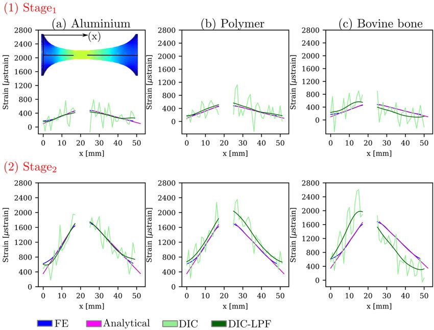
www.nature.com/scientificreports/
Various studies examined the accuracy of DIC strain measurements and showed that the strain on the meas-
ured surfaces can be overestimated9,15,23,27. The precision of DIC measurements is acceptable when specimens
are deforming in the linear-elastic region, but after yielding the standard deviation increases v astly36,37. Two
options could be employed for investigating the accuracy of DIC strain measurements, either by verifying the
measurement at the position of measurement d evice24,27,38–40, or by means of finite element (FE) models for the
full-field strain distribution8,9,12. Despite the high accuracy of SGs and extensometers, their measurement is
limited to a single point, and can be compared to DIC measurements only by averaging the full-field data over
the SG area15,39,41, which is only advantageous for homogeneous strain fields. In contrast, FE models can give
accurate prediction of the full-field strain measurements, but it is important to know the geometry, material
behaviour and boundary conditions. With knowledge of these parameters FE models are a suitable way to evalu-
ate strain non-homogeneity12,42,43. For example, Liu et al.12, investigated experimentally the strain concentration
on hydrogel specimens in the presence of large strain gradients, they found a very good agreement between the
FE results and the measured DIC full-field strain, however, 2D DIC was employed which is less useful for objects
with curvatures, like the human femur.
Non-homogeneous strain fields were measured on the surface of biological t issues24,27,44,45. For example, on
the neck of the human femur, the normalized strain gradient changes by about 7% per mm on average (more in
the next section). DIC measurements is advantageous not only for measuring non-homogeneous strain fields,
but also for measuring strain gradients46–48. Various studies reported DIC full-field strains without reporting the
accuracy of the measurement or validating it against another method, Tsirigotis et al.49 found that the surface
strain, on bovine cancellous bone under compression load, showed steep strain gradients. Likewise, Palanca
et al.50 and Grassi et al.51 measured full-field surface strain on the superior neck of human femurs. However, the
strain results were not validated against another measurement method, and Tsirigotis et al.49 used 2D DIC. Many
DIC strain measurements on different bone models were verified using SGs only, and were used to verify FE
models22,27,38,52,53. Despite the numerous studies on the accuracy of DIC measurements, only one study, Baldoni
et al8, verified linear experimental full-field DIC strain measurement, the verification was against the theoretical
solution and not against another measurement technique, and the strain gradient was not analyzed.
Other studies focused on testing the accuracy of DIC numerically. For instance, Wang et al.11, tested the
accuracy of 2D DIC for non-homogeneous strains of numerically deformed images, they found that the uncer-
tainty of DIC increases around the strain concentration regions,here the reference images were also captured
by one camera only (2D DIC), and numerically deforming the images excludes the errors originated from the
experiment’s environment. A verification of 3D DIC measurements for linear strain fields and strain gradients
experimentally is still missing. To verify non-homogeneous strain fields measured by DIC, the strain gradients
on the specimen’s surface must be known. Non-homogeneous strain fields such as linear or quadratic strain
fields are good candidates since the analytical (theoretical) solution can be calculated beforehand. This study is
focusing only on linear strain fields.
The objective of this study is to design a novel specimen shape where a well-defined linear gradient field can
be measured and to investigate the accuracy of DIC full-field strain measurement globally and locally. This is
the first study to systematically evaluate and validate non-homogeneous DIC strain measurements on surfaces
where strain gradients are expected on biological and engineering materials. Measurements are done with a 3D
DIC system and the noise in the DIC strain fields is reduced by applying Gauss low-pass filtering with optimal
cutoff frequency. SGs are used to measure the experimental strain at pre-defined positions, which was compared
to the DIC strain measurement locally. Summarizing, this work aims at verifying whether DIC measurements
can capture gradient fields and local normalized strain gradients at specific positions in case of bone and for
comparison purposes on typical engineering materials (aluminium and polymer).
Materials and methods
Normalized strain gradient. To explore the capability of a DIC system to measure linear strain fields on
the surface of the test specimens, it is necessary to design a specimen shape where the strain on the surface of the
specimen changes linearly during deformation. Different options are available to design such a specimen, either
by changing the width or the thickness of the test specimen. In this study, it is intend to measure strain gradient
magnitudes similar to that found on a surface of a proximal human femur. For this purpose, a load and size inde-
pendent measured value - a normalized strain gradient - is defined. This is based on a normalized strain εnorm
which is the difference between the strain at two points divided by their average quantity [Eq. (1)]. The gradient
is obtained by dividing this normalized strain by the distance of these two points (Eq. (2)).
|εp1 − εp2 |
εnorm = εp1 +εp2 (1)
2
εnorm 1
εnorm grad = (2)
d mm
where εp1 and εp2 in this work are equivalent strains εeq which are measured at two locations p1 and p2 on the
femur, and d is the distance between the two points (see in Appendix A, Supplementary Fig. 1 shows a SED map
of a proximal femoral under physiological load54). The equivalent strain εeq is obtained from the local strain
energy density (SED) and elastic modulus (10 GPa) as follows:
Scientific Reports | (2021) 11:17515 | https://doi.org/10.1038/s41598-021-97085-x 2
Vol:.(1234567890)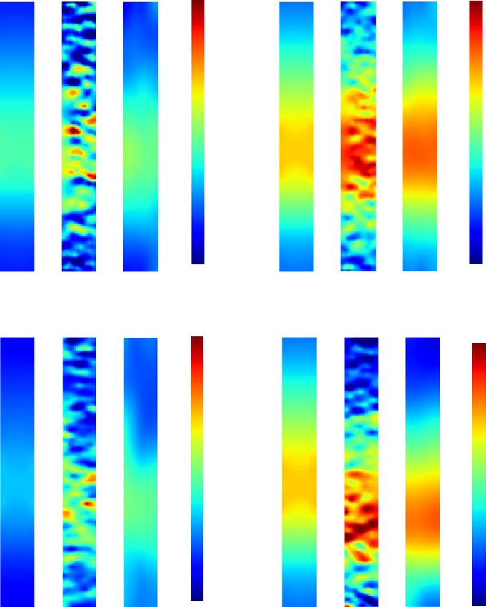
www.nature.com/scientificreports/

                                  Figure 1.  (a) Specimen’s geometry derived from Eq. (12), w(x) shows how the curvature of the specimen
                                  changes; in red and blue the high- and low-gradient ROIs are shown, respectively. L1 is the high-gradient ROI
                                  and where SG1 is placed. L2 is a neutral ROI connecting the high-gradient ROI with the low-gradient ROI, L2
                                  shows constant strain and where SG2 is placed. L3 is the low-gradient ROI and where SG3 is placed. (b) The
                                  theoretical strain distribution along the specimen’s length. The high- and low-strain gradients are shown in red
                                  (steeper curve) and blue, respectively. Constant strain (in green) connects both gradient regions.


                                                                                                  2SED
                                                                                     εeq =                                                        (3)
                                                                                                    E
                                      For the human femur, the normalized strain gradient is about 3.5 and 7.2% per mm on average in the head
                                  and neck regions, respectively (see Appendix A, Supplementary Table 1). This work aims to design a specimen
                                  shape which under deformation gives a linear strain field, and where two normalized strain gradients of around
                                  3.5 and 7% per mm (regardless of the load applied) can be found on the surface.

                                  Analytical strain and specimen shape. A linear field in a tensile specimen can be generated by a specific
                                  specimen shape. In the following derivations we calculate the specimen shape. The exact strain distributions for
                                  comparison with DIC are determined by means of FE.
                                      In the following uniaxiality is assumed, w(x) is the width (shape) of the specimen, and ε(x) is the strain along
                                  x, see Fig. 1a and b. A one-dimensional linear strain field can be written as:
                                                                                     ε(x) = a + bx                                                (4)
                                  where a is a point on the specimen where the strain shows the far field value, b is the slope of the linear strain
                                  and x is a position along the specimen’s axis, see Fig. 1. Solving for a and b at the positions 0 and L gives:
                                                                                 at x = 0 :       ε(0) = a                                        (5)

                                                                    at x = L :       ε(L) = ε(0) + b · L = ε(0) · k                               (6)
                                  where the maximum strain ε(L) can be linked to the far field strain ε(0) by a concentration factor k. Solving for
                                  the slope of the linear equation, b:
                                                                                        ε(0)
                                                                                   b=        · (k − 1)                                            (7)
                                                                                         L
                                      The strain at any point between a and L can be calculated via inserting a and b in Eq. (4):
                                                                            ε(0)                                    x
                                                              ε(x) = ε(0) +      · (k − 1) · x = ε(0) 1 + (k − 1) ·                               (8)
                                                                              L                                      L
                                      Due to the asymmetric specimen shape as shown in Fig. 1, two different strain gradients can be realized. For
                                  example, if ε(0), L and k are prescribed, the strain function and the normalized strain gradient [Eq. (2)] along
                                  the specimen’s length can be computed. The normalized strain gradient changes between 4.4 and 22% per mm,
                                  and between 3 and 14% per mm for specimen’s length of 18 and 27 mm, respectively. Two positions were selected
                                  relatively close to the middle of the specimen for the normalized strain gradients investigation. These are the
                                  nearest values to the two normalized strain gradients found on the surface of the human femur (3.5 and 7.3%
                                  per mm), which are 3.6 and 6.9% per mm for a specimen’s length of 18 and 27 mm, respectively.
                                      The unknown width of the specimen w(x) follows from the equilibrium i.e. the force experienced along the
                                  specimen’s length is constant at one loading stage:

Scientific Reports |   (2021) 11:17515 |               https://doi.org/10.1038/s41598-021-97085-x                                                    3

                                                                                                                                               Vol.:(0123456789)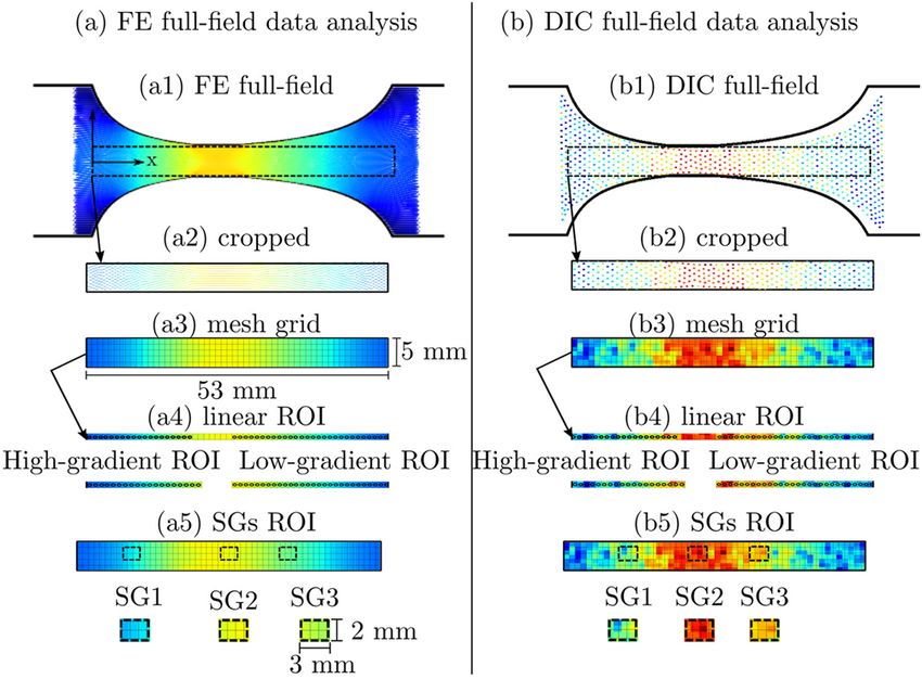
www.nature.com/scientificreports/
F(0) = F(x) (9)
Therefore, the equation can be rewritten in terms of stress (σ = E · ε) and cross-sectional area ( A = 2w(0) · t):
E · ε(0) · 2w(0) · t = E · ε(x) · 2w(x) · t (10)
where t is the thickness of the specimen (which is constant), w(0) is the half-width of the specimen and equals
12.5 mm, see Fig. 1a. Equation (10) can be rewritten as:
ε(0) · w(0)
w(x) = (11)
ε(x)
Solving for w(x):
ε(0) · w(0) w(0)
w(x) =
= x (12)
ε(0) L+(k−1)·x 1 + (k − 1) · L
L
Figure 1a shows the specimen’s geometry for k = 5 by plotting w(x) from Eq. (12) for two lengths, in red and
blue in Fig. 1a. The size limitation in this work was on the one hand the specimen width of 25 mm for bone and
on the other hand the specimen width of 5 mm in SG2 ROI for the application of SG2. The overall length of the
specimen was 193 mm for aluminium and polymer specimens and was 73 mm for bovine bone specimens. The
length of the Region of Interest (ROI) is 53 mm and is divided into three regions (L1, L2 and L3). L1 is 18 mm
long (high-gradient ROI, showing 6.9% per mm normalized strain gradient), L2 is 8 mm long (constant strain,
no gradient), and L3 is 27 mm long (low-gradient ROI, showing 3.6% per mm normalized strain gradient). In
these three regions, three SGs are applied at specific locations. Three ROIs are investigated in this study: the
high- and low-gradient ROIs and the SGs ROIs. Figure 1b shows the linear strain (in red and blue) along the
shape of the specimen.
SGs strain. Strains were recorded with one-element, 120-ohm rectangular strain gauge (K-CLY4-0030-
1-120-3-020, HBM, Darmstadt, Germany). The strain in the loading direction was recorded (acquisition fre-
quency 5 Hz) using a QuantumX data acquisition (HBM, Darmstadt, Germany).
The positions of the three SGs are depicted in Fig. 1. SG2 was applied at L2 where the strain is constant. This
strain was used to calibrate the FE models as described below for the FE model. SG1 and SG3 were applied where
the normalized strain gradient is 6.9 and 3.6% per mm, which as explained above can be found on the surface
of the femoral neck and head, respectively.
Numerical strain (FE model). The analytical strain field from Eq. (8) does not consider the Poisson effect.
To check the analytical model and verify the accuracy of the DIC measured strains, FE models were gener-
ated to provide accurate strains. The FE models were created for each specimen using an open source Calculix
solver (PrePoMax, v0.6.0). The specimens’ geometry are as shown in Fig. 1a. The specimens were meshed with
tetrahedral (C3D10) second-order elements of the size 0.8 mm, see Fig. 2. To scale the FE strain to the strain
measured by SG2, 1 mm displacement (ux ) was imposed on the specimen simulating a uniaxial tensile test in the
x-direction. The obtained FE strain was scaled so that the FE strain is equal to the strain in SG2. This is possible
because of the linear elastic system.
DIC strain measurements. DIC computes full-field strain on the surface of the specimen. More informa-
tion is available here17 on how DIC computes strain. For this study, the surface strain was computed with a facet
(subset) size of 19 × 19 pixels and a facet step of 16 pixels (50% overlapping), these parameters are recommended
by the manufacturer for 6 Megapixel CCD cameras. The strain in the loading direction were exported from the
ARAMIS Professional software (v6.3.1; GOM GmbH, Germany) along the node number (> 600 measurement
points) and x-, y-, z-coordinates, for plotting and post-processing with Python SciPy.
Specimen preparation. The specimen shape was produced in aluminium (ALMG3 (AW-5754)) (n = 5),
polymer (Polyacetal POM-Copolymer) (n = 5) and Bovine bone (n = 5). Aluminium and polymer specimens
were manufactured by means of a numerical controlled machine (CNC Router BZT PFX 700, BZT Maschinen-
bau GmbH, Leopoldshöhe, Germany) from aluminium and polymer plates of 1.5 mm and 4 mm thickness,
respectively.
For bovine bone, two fresh compact femurs of bovines (18–24 months old) were obtained from the local
butcher. The mid-diaphysis of the femur was cut, the hollow cylinder of the femur shaft was then cut into rough
rectangular beams using a hand saw. After that, the beams were embedded into epoxy mould which was then
fixed into a CNC machine to obtain the shape of the specimen. Finally, using a slice cutting machine (Exakt 300
CL Band System, EXAKT Advanced Technologies GmbH, Norderstedt, Germany) longitudinal specimens were
sliced (thickness of 2 mm), see Fig. 3a. During the whole preparation steps and until testing, the bone specimens
were kept wet with phosphate buffered saline (PBS) solution and when not used, the specimens were preserved
in a − 20 °C freezer.
Three SGs were applied on one face of the test specimen as in Fig. 3b while the other face was covered with
paper tape to protect it against any glue resins during the SGs’ application. First, using a light microscope, the
position of the SG was precisely marked on the surface of the specimen. Second, two component glue (Methyl
methacrylate, HBM, Darmstadt, Germany) were mixed and applied on the bone surface and then each SG was
Scientific Reports | (2021) 11:17515 | https://doi.org/10.1038/s41598-021-97085-x 4
Vol:.(1234567890)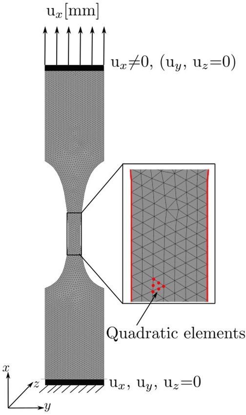
www.nature.com/scientificreports/
Figure 2. FE model including boundary conditions and mesh. The displacement was applied on the top of the
specimen, while the bottom was constrained to mimic the experimental conditions. No material parameters
(Elastic modulus) were assigned to the specimens because only strains were calculated and the FE simulation is
displacement control. A poisson’s ratio of 0.3 was assigned for all specimens.
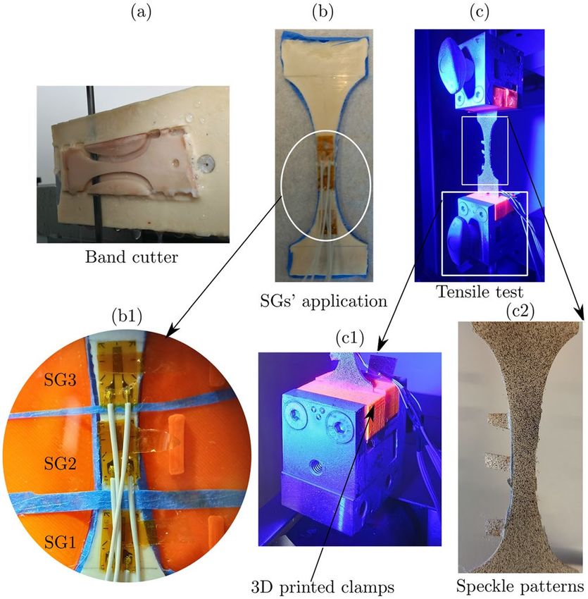
Figure 3. Preparation steps of the bovine bone specimens. (a) Bone specimens were sliced using an Exakt
cutter, (b) SG1, SG2 and SG3 were applied on the specimen’s back, (c) mechanical test setup, (c1) the bone
specimen was fixed to external clamps, and (c2) speckle patterns were applied on the specimen’s front.
Scientific Reports | (2021) 11:17515 | https://doi.org/10.1038/s41598-021-97085-x 5
Vol.:(0123456789)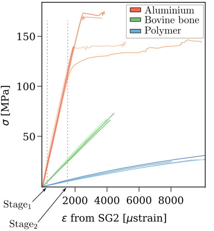
www.nature.com/scientificreports/

                                            Figure 4.  RMSE computational method. (a, b) FE and DIC full-field data analysis respectively, (a1, b1) the
                                            full-field surface strain from FE and DIC, (a2, b2) cropping of the linear regions excluding the boundary nodes,
                                            (a3, b3) a 53 mm × 5 mm mesh grid for aligning the measurement points into a regular grid, (a4, b4) the high-
                                            and low-gradient ROIs from the middle line along the specimen’s length were extracted, (a5, b5) SGs ROIs were
                                            cropped at SG1 and SG3.

                                            carefully applied. Each specimen was then fixed to external clamps by gluing the specimen to 3D printed parts
                                            using 5 mins two components epoxy (Fiber-reinforced composite, Waldenbuch, Germany) as in Fig. 3c1. Speckle
                                            patterns were applied to the other surface using a high precision airbrush (Profi-AirBrush, Germany), as shown
                                            in Fig. 3c2. The airbrush settings were adjusted (air pressure of 150 kPa, 3 turns of the airbrush opening, and 9 cm
                                            distance between the airbrush and the specimen) to obtain a speckle size of 3−5 pixels with a random distribu-
                                            tion (coverage 45–50%)5. Finally, the specimen was clamped to the tensile testing machine and was exposed to
                                            the blue light for the DIC system see Fig. 3c. Similar procedure was followed for the aluminium and polymer
                                            specimens, only another glue (Cyanoacrylate, HBM, Darmstadt, Germany) was applied to fix the SGs on the
                                            specimens’ surface as recommended by the manufacturer of the SGs.

                                            Mechanical tests. The test specimens were mounted on a Zwick (Z030) machine (ZwickRoell GmbH, Ger-
                                            many) with force cell up to 30 kN. 3D DIC system (ARAMIS 150/6M/Rev.02,GOM, Braunschweig, Germany)
                                            was set up with two CCD cameras. The cameras were positioned perpendicular to the specimen at 35 cm dis-
                                            tance. The SGs cables were welded to an adaptor (full-bridge) which was connected to a QuantumX DAQ device
                                            (HBM, Darmstadt, Germany) for data acquisition. Finally, the specimens were subjected to a uniaxial tensile
                                            load along the vertical direction (displacement control) with cross-head movement of 0.5 mm/min till fracture.
                                            The acquisition rate was synchronized between the SG’s and the DIC system at 5 Hz.

                                            Data evaluation.        In this study, the strain measurements were defined over three ROIs: high- and low-
                                            gradient ROI, and SGs ROIs, see Fig. 4. The scaled full-field strain obtained from the FE model is considered as
                                            the reference strain. At the high- and low-gradient ROIs, the accuracy of the DIC strain measurements and the
                                            analytical strain computation are evaluated by means of the root mean square error (RMSE). At the SGs ROIs,
                                            the two experimental strains form DIC and the SGs are compared statistically, and the normalized strain gradi-
                                            ents (6.9 and 3.6% per mm) are computed and compared to the reference obtained from FE.
                                               Figure 4 shows the computational method of the RMSE:

                                            • The full-field strain (Fig. 4a1, b1) obtained from both FE and DIC, respectively. They were cropped horizon-
                                              tally and vertically based on the x- and y- coordinates.
                                            • The cropped fields were interpolated into a regular mesh grid of (53 mm × 5 mm) points, see Fig. 4a3, b3) to
                                              be able to compare values.
                                            • The middle line of the interpolated fields was exported into a 1D matrix, see Fig. 4a4 and b4 for line plots
                                              along the centre of the specimen.
                                            • The positions of the three SGs were cropped from the (53 mm × 5 mm) mesh grid for SG size of 3 mm × 2
                                              mm, see Fig. 4a5 and b5 to compare values inside the SG region.
                                            • The RMSE was calculated for the high- and low-gradient ROIs.

                                            The RMSE equation is:

                                                                                                   1 n FE                2
                                                                              RMSEMethod =           �i=1  εi − Method εi                                  (13)
                                                                                                   n

          Scientific Reports |   (2021) 11:17515 |               https://doi.org/10.1038/s41598-021-97085-x                                                   6

Vol:.(1234567890)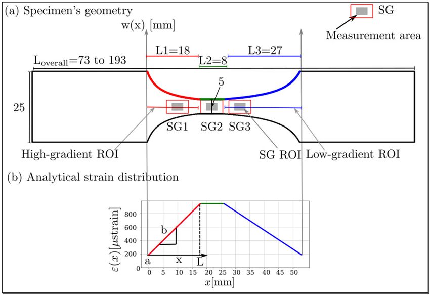
www.nature.com/scientificreports/
Figure 5. Stress–strain curve of all tested specimens. Aluminium in red, bovine bone in green and polymer in
blue. The error evaluation was done at two deformation stages, approximately at 500 μstrain and 1750 μstrain.
Five specimens were tested from each material.
where RMSEMethod refers to the RMSE computed for each method, i.e. RMSEDIC is the RMSE of the DIC strain
measurements compared to FE strains, n is the number of strain measurement points (i) in a ROI, FE εi is the
value of the reference strain (FE), εi is the value of the analytical or DIC strains.
The RMSE was evaluated at two deformation stages, hereinafter referred as ( Stage1 and Stage2 ). Stage1 is
at approximately 500 μstrain, a low strain level similar to the noise level of the DIC measurement. Stage2 is at
approximately 1750 μstrain level which is found during normal ambulation and is comparable for bone defor-
mation under physiological load55. Because the exact values of 500 and 1750 μstrain were not found in all the
measurements of SG2 for all the test specimens, the nearest measurement points to 500 or 1750 μstrain were
selected which were about 496 and 1698 μstrain, respectively. The nearest point had a difference of less than 3%
to 500 or 1750 μstrain.
To answer the question of how well the local strain gradient can be captured with DIC compared to FE, the
two normalized strain gradients (6.9 and 3.6% per mm) are computed as in Eq. (2). Basically, along the speci-
men’s axis, first the normalized strain [Eq. (1)] is computed by dividing the difference in strain measurement
between two measurement points by their average quantity. Then, the normalized strain gradient is computed
by dividing the normalized strain by the distance between the two measurement points, 2 mm.
Noise reduction. Gaussian low-pass filter (LPF) with cutoff frequency of 2.5, which was found as the opti-
mal cutoff frequency in our previous study17, was applied on the DIC full-field strain measurements to reduce
the noise in the DIC strain measurements. The same cutoff frequency was applied on all stages independent of
the load applied.
Results
Mechanical testing. The stress–strain curves of all tested specimens (five of each material), with strain
obtained from SG2 (constant strain) are shown in Fig. 5. The two vertical dashed lines show the deformation
stages (Stage1 and Stage2) at which the results were evaluated.
From the stress–strain curve, the elastic modulus was computed for the tested materials and it was on aver-
age 71.37 ± 2.03, 3.24 ± 0.25, and 16.92 ± 0.61 GPa for aluminum, polymer, and bovine bone, respectively (for
more details, see Appendix B, Supplementary Table 2 lists the elastic modulus for all specimens. For bovine
bone, results of the elastic modulus are in agreement with values found in the literature for cortical bone56–58).
RMSE for the high‑ and low‑gradient ROIs. The RMSE was evaluated for the high- and low-gradient
ROIs, as shown in Fig. 4c1 and c2. Figure 6 shows the two ROIs plotted along the specimen’s length at two
deformation stages (Stage1 and Stage2). For aluminium and polymer, there is a good agreement between the FE
strain, the analytical strain and the filtered DIC strain. For bovine bone, the DIC strain overestimated the strain
in the high-gradient ROI at both deformation stages, in contrast to the low-gradient ROI where DIC strain
underestimated the strain in comparison to FE strain. In all curves, the LPF successfully reduced the noise (the
fluctuations) in the DIC strain measurements.
Figure 7 depicts the RMSE for the linear strain gradients ROIs at Stage1 and Stage2 for the three tested materi-
als. The RMSEanalytical deviated by less than 60 μstrain from the reference FE strain for all the tested materials.
The RMSEDIC was about 400 μstrain when compared with the FE strain. Filtering of the DIC fields had a positive
effect on the RMSE where it was reduced on average by 63% at Stage1 and by 34% at Stage2.
Two-dimensional visualization of the full-field strains from FE and DIC are depicted in Fig. 8 for (a) one
polymer and (b) one bovine bone specimens (The results of all the tested specimens are shown in Appendix
Scientific Reports | (2021) 11:17515 | https://doi.org/10.1038/s41598-021-97085-x 7
Vol.:(0123456789)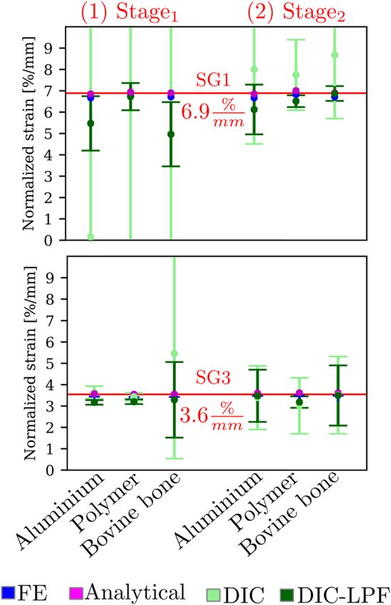
www.nature.com/scientificreports/

                                            Figure 6.  Full-Field linear strains at the two deformation stages, for (a) aluminium, (b) polymer, and (c) bovine
                                            bone. The strain is plotted along the specimen’s ROI (53 mm), the strain was obtained from the high- and low-
                                            gradient ROIs, as in Fig. 5a4 and b4. The FE, analytical, DIC and DIC filtered strain are plotted in blue, magenta,
                                            light-green and dark green, respectively. DIC-LPF refers to the DIC strain fields after Gaussian LPF was applied.

                                            Figure 7.  RMSE for the linear strain gradients ROIs at the two deformation stages for the three tested materials.

          Scientific Reports |   (2021) 11:17515 |               https://doi.org/10.1038/s41598-021-97085-x                                                   8

Vol:.(1234567890)
www.nature.com/scientificreports/
Figure 8. Two-dimensional visualization of the DIC full-field strain measurements of one polymer and one
bovine bone specimens. At both deformation stages; the reference strain from the FE model for this specific
specimen, the DIC strains (original and filtered) are shown.
C, Supplementary Fig. 2). Linear changes in the strain field cannot be recognized at Stage1. On the contrary, at
Stage2, the linear strain field can be recognized, but corrupted with noise, which was then reduced when Gaussian
LPF was applied. It is worth noting that the DIC strain fields shown in Fig. 8 are the raw data from the ARAMIS
software without the application of any filtering, neither when the surface component was created, nor when
the strain was calculated. The DIC-LPF fields are the DIC fields after the application of the Gaussian LPF using
an in-house algorithm.
Normalized strain gradient at SGs ROIs. At the positions of the SGs, the corresponding FE and DIC
strains were cropped as shown in Fig. 4a5 and b5. Figure 9 shows the normalized strain gradient at the positions
of SG1 (6.9% per mm) and SG3 (3.6% per mm).
At SG1 (high-gradient), the DIC normalized strain gradient fails severely (with maximum difference to 6.9%
per mm exceeding 90%) at Stage1 and fails moderately (with maximum difference to the reference of 25%) at
Stage2. After applying the Gaussian LPF (depicted in dark green), the normalized strain gradients were success-
fully retrieved for most of the cases (maximum difference is 20% for aluminium and bovine bone).
In contrast, at SG3 (low-gradient), the average DIC normalized strain gradient and the standard deviation
were closer to the reference strain for Stage1 and Stage2, except for bovine bone at Stage1. As well, Gaussian LPF
improved the detection of the normalized strain gradients (with maximum difference to the reference of 12%).
Finally, the two experimental strain measurements obtained from DIC and SGs were compared. Table 1 lists
the average strain obtained from DIC (at the SG’s position) and the SG’s recorded strain at Stage1 and Stage2.
The average of the standard deviations exceeded 50% for DIC measurements at Stage1 where the signal to noise
ratio is lowest. One aluminium sample had a very low reading of SG1 at Stage1 which resulted in a high standard
deviation. A paired-specimens t-test ( α = 0.05) was conducted to compare the strain recorded by the SGs and
their average corresponding area from DIC. For the majority of the measurements, no significant difference was
found between the SGs and the DIC measurements (Statistical summary of the Shapiro-wilk and the t-test can be
found in Appendix D, Supplementary Tables 3 and 4). Additionally, the precision of the DIC strain measurement
did not change largely and remained between 190 μstrain and 360 μstrain for the different deformation stages.
Discussion
The main goals of this study were to examine the capability of a 3D DIC system to measure a linear strain field
on the surface of a newly designed gradient test specimen, with and without filtering.
Scientific Reports | (2021) 11:17515 | https://doi.org/10.1038/s41598-021-97085-x 9
Vol.:(0123456789)www.nature.com/scientificreports/
Figure 9. The normalized strain gradients at SG1 (6.9% per mm) and SG3 (3.6% per mm) is plotted for two
deformation stages for aluminium, polymer, and bovine bone. The normalized strain gradient was calculated
according to Eq. (2).
Aluminium Polymer Bovine bone
SG Stage SG DIC SG DIC SG DIC
SG1 217 ± 215 314 ± 193 358 ± 32 260 ± 143 440 ± 115 298 ± 229
SG2 Stage1 494 ± 7 484 ± 270 497 ± 5 496 ± 172 489 ± 3 544 ± 302
SG3 369 ± 62 459 ± 280 416 ± 54 376 ± 214 472 ± 69 429 ± 203
SG1 979 ± 398 1055 ± 252 1224 ± 106 1212 ± 236 1329 ± 399 1058 ± 362
SG2 Stage2 1748 ± 16 1764 ± 224 1743 ± 6 2157 ± 186* 1745 ± 5 1774 ± 276
SG3 1306 ± 147 1503 ± 247 1438 ± 162 1594 ± 227 1775 ± 88 1513 ± 187
Table 1. Average strain measurements ± standard deviation for the DIC and SGs at the three SGs’ positions.
All listed values are in μstrain. The standard deviation for the DIC measurements is the average of the different
standard deviations for the measured specimens. *Indicates a significance difference in the mean.
Two strain measurement (SGs and DIC) and two strain computational (analytical and FE) methods were
employed in this study. The RMSE was evaluated for the high- and low-gradient ROIs at two deformation stages,
and the gradient was verified by a newly defined normalized strain gradient measure.
Due to the noise in the DIC strain measurement, the DIC strain deviated (RMSEDIC < 500 μstrain) from the
FE strain - the gold standard in this study - for both the high- and low-gradient ROIs. Gaussian LPF successfully
reduced the noise in the DIC full-field strain measurements for all the tested materials. However, the overall
reduction in noise can be seen as reduction of the fluctuations of each field rather than reducing the overall meas-
urement values. At Stage1 and Stage2, the RMSEDIC was reduced on average by 63% and 34%, respectively. In total,
filtering reduced the RMSE to less than 200 μstrain which is in line with values reported in the literature8,22,32,59.
The main interest in this work is to examine the capability of DIC to measure strain gradients. For this, two
engineering materials, stiffer (aluminium) and softer (polymer) than bone, were chosen for this investigation.
At the location of high normalized strain gradient (6.9% per mm), only with applying Gaussian LPF the normal-
ized strain gradient was retrieved. In contrast, at the location of low normalized strain gradient (3.6% per mm),
the normalized strain gradient was measured accurately for all cases except for bovine bone, which was then
improved when the LPF was applied. The normalized strain gradient is an indicator for how good can the DIC
Scientific Reports | (2021) 11:17515 | https://doi.org/10.1038/s41598-021-97085-x 10
Vol:.(1234567890)www.nature.com/scientificreports/
strain measurements measure local variation in the strain fields. In the examined cases, the accuracy of such
a value was demonstrated to be higher for low strain concentrations. This can be helpful for measuring strain
concentration on the surface of the human femur. However, one should be aware that to decide whether such
a value is accurately measured or not, a reference value or an idea of the strain concentration must be known.
Taking a closer look at these analysis, one could look at the DIC full-field strain measurements (see Appendix
C, Supplementary Fig. 2). Linear strain fields were not recognized on the surface of all tested specimens. For engi-
neering materials, the deviation from the reference FE was less evident than for the bovine bone specimens, where
shifts in the linear strain fields were observed. These shifts can be attributed to the local variations of material
and structural properties of bone i.e. the orthotropy of the material or the bone texture. During bone specimen
preparation, pores (holes) were visible under the light microscope on the test surface. These holes, originated
from blood vessels canals or trabecular bone, influenced the DIC measurements. It might be helpful to reduce
the surface roughness by grinding the specimens, however, with grinding, pores might disappear or increase in
size and new pores might appear. The non-homogeneity in the measured strain on bone surface was detected by
Grassi et al.51 who showed that DIC measured strain localization in proximity of cortical pores of the proximal
femur. As well as Katz et al.41 who showed that holes affected the strain pattern in the DIC measurements and
that FE models should consider these holes. This non-homogeneity in the material besides the anisotropic nature
of bone contributed to the variations in the DIC strain measurements. It would be useful for future studies to
include pores in the FE analysis or create FE models based on geometries obtained from scanned specimens.
There was no significant difference in means between the averaged DIC strain measurement over the SG’s
locations and the SGs strain for the majority of the cases. However, no significant difference does not necessarily
mean accurate, no clear over- or underestimation were recognized of the DIC measurements. Similar results
were found in the literature that validated DIC measurements with SGs or FE models9,15,22,23. All these studies
suggest that DIC strain measurement should be examined for accuracy. It is obvious that non-consistent errors
were found in the DIC measurements, which empathizes the need for validation and optimization to maintain
the error at minimum levels.
In summary, this study provided an unprecedented insight into the measurement accuracy of linear strain
fields on the surface of different materials by means of DIC. A new innovative specimen shape with two gra-
dients was presented which can be further developed and adapted for different strain gradients and tests with
different DIC systems. With the normalized strain gradient, it was possible to measure and verify local strain
concentrations which is due to the specimen shape their magnitude were known a priori. This study showed that
DIC systems can be optimized for non-homogeneous strain fields such as strains found on the surface of many
biological tissues and structures. The normalized strain gradient is essential to understand the range of strain
changes per unit mm on the surface of bone. Finally, the common practice of averaging the strain measured on
bone surface is not optimal since many strain concentration locations get homogenized.
Limitations of this study are, only one facet and grid size were used as recommended by the DIC software,
changing the facet and the grid size to smaller ones would definitely increase the density of the DIC measured
points, but at the cost of more n oise11,15,59,60. Optimal filter parameter found in our previous s tudy17 was applied,
however, other filter strategies might be useful to reduce the error in DIC strain measurements such as pre-
filtering of the speckled images14. Finally, the strain gradients values were evaluated for one human proximal
femur at physiological load, it might be useful to evaluate strain concatenations beyond the physiological load.
Conclusion
The normalized strain gradient found on the proximal femur under physiological load was the basis for design-
ing the specimens tested in this work. It was possible to capture such gradients with DIC. Gaussian low-pass
filtering reduced the noise found in the DIC measurements and highly improved the detection of the normal-
ized strain gradients. The outcome was better for (1) a lower normalized strain gradient, (2) higher strain level,
(3) engineering materials. Beside this finding, the study provides a new specimen design and methodological
approach for investigating non-homogeneous full-field strains with DIC on engineering but also hard biological
tissues like bone.
Received: 22 June 2021; Accepted: 13 August 2021
References
1. Avril, S., Pierron, F., Sutton, M. A. & Yan, J. Identification of elasto-visco-plastic parameters and characterization of lüders behavior
using digital image correlation and the virtual fields method. Mech. Mater. 40, 729–742 (2008).
2. Liu, X. & Lu, R. Testing system for the mechanical properties of small-scale specimens based on 3d microscopic digital image
correlation. Sensors 20, 3530 (2020).
3. Versaillot, P. D., Wu, Y.-F. & Zhao, Z.-L. Experimental study on the evolution of necking zones of metallic materials. Int. J. Mech.
Sci. 189, 106002 (2021).
4. Xu, Z., Peng, L., Jain, M. K., Anderson, D. & Carsley, J. Local and global tensile deformation behavior of aa7075 sheet material at
673ok and different strain rates. Int. J. Mech. Sci. 195, 106241 (2021).
5. Lecompte, D., Bossuyt, S., Cooreman, S., Sol, H. & Vantomme, J. Study and generation of optimal speckle patterns for DIC. Proc.
Annu. Conf. Exposit. Exp. Appl. Mech. 3, 1643–1649 (2007).
6. Lionello, G. & Cristofolini, L. A practical approach to optimizing the preparation of speckle patterns for digital-image correlation.
Meas. Sci. Technol. 25, 107001 (2014).
7. Palanca, M., Tozzi, G. & Cristofolini, L. The use of digital image correlation in the biomechanical area: A review. Int. Biomech. 3,
1–21 (2016).
Scientific Reports | (2021) 11:17515 | https://doi.org/10.1038/s41598-021-97085-x 11
Vol.:(0123456789)www.nature.com/scientificreports/
8. Baldoni, J., Lionello, G., Zama, F. & Cristofolini, L. Comparison of different filtering strategies to reduce noise in strain measure-
ment with digital image correlation. J. Strain Anal. Eng. Des. 51, 416–430. https://doi.org/10.1177/0309324716646690 (2016).
9. Hensley, S. et al. Digital image correlation techniques for strain measurement in a variety of biomechanical test models. Acta
Bioeng. Biomech. 19, 187–195 (2017).
10. Yaofeng, S. & Pang, J. H. Study of optimal subset size in digital image correlation of speckle pattern images. Opt. Lasers Eng. 45,
967–974 (2007).
11. Wang, Y. et al. Investigation of the uncertainty of DIC under heterogeneous strain states with numerical tests. Strain 48, 453–462
(2012).
12. Liu, M., Guo, J., Hui, C.-Y. & Zehnder, A. Application of digital image correlation (dic) to the measurement of strain concentration
of a pva dual-crosslink hydrogel under large deformation. Exp. Mech. 59, 1021–1032 (2019).
13. Rajan, V., Rossol, M. & Zok, F. Optimization of digital image correlation for high-resolution strain mapping of ceramic composites.
Exp. Mech. 52, 1407–1421 (2012).
14. Pan, B. Bias error reduction of digital image correlation using gaussian pre-filtering. Opt. Lasers Eng. 51, 1161–1167 (2013).
15. Acciaioli, A., Lionello, G. & Baleani, M. Experimentally achievable accuracy using a digital image correlation technique in measur-
ing small-magnitude (less than 0.1%) homogeneous strain fields. Materials 11, 751 (2018).
16. Hoult, N. A., Take, W. A., Lee, C. & Dutton, M. Experimental accuracy of two dimensional strain measurements using digital
image correlation. Eng. Struct. 46, 718–726 (2013).
17. Amraish, N., Reisinger, A. & Pahr, D. H. Robust filtering options for higher-order strain fields generated by digital image correla-
tion. Appl. Mech. 1, 174–192 (2020).
18. Iarve, E. & Pagano, N. Singular full-field stresses in composite laminates with open holes. Int. J. Solids Struct. 38, 1–28 (2001).
19. Lagattu, F., Lafarie-Frenot, M., Lam, T. & Brillaud, J. Experimental characterisation of overstress accommodation in notched cfrp
composite laminates. Compos. Struct. 67, 347–357 (2005).
20. Pan, B., Wang, Z. & Lu, Z. Genuine full-field deformation measurement of an object with complex shape using reliability-guided
digital image correlation. Opt. Express 18, 1011–1023 (2010).
21. Janíček, P., Blažo, M., Navrátil, P., Návrat, T. & Vosynek, P. Accuracy testing of the dic optical measuring method the aramis system
by gom. in 49th International Scientific Conference, 139 (2011).
22. Dickinson, A., Taylor, A., Ozturk, H. & Browne, M. Experimental validation of a finite element model of the proximal femur using
digital image correlation and a composite bone model. J. Biomech. Eng. 133, 014504. https://doi.org/10.1115/1.4003129 (2011).
23. Gilchrist, S., Guy, P. & Cripton, P. A. Development of an inertia-driven model of sideways fall for detailed study of femur fracture
mechanics. J. Biomech. Eng. 135, 121001 (2013).
24. Grassi, L. et al. Full-field strain measurement during mechanical testing of the human femur at physiologically relevant strain
rates. J. Biomech. Eng. 136, 111010 (2014).
25. Venkatesan, S. et al. A study on the real time strain measurement system for analysis of strain evolution and failure behavior of
cortical bone materials. Mater. Forum 33, 1–10 (2009).
26. Sztefek, P. et al. Using digital image correlation to determine bone surface strains during loading and after adaptation of the mouse
tibia. J. Biomech. 43, 599–605 (2010).
27. Begonia, M., Dallas, M., Johnson, M. L. & Thiagarajan, G. Comparison of strain measurement in the mouse forearm using subject-
specific finite element models, strain gaging, and digital image correlation. Biomech. Model. Mechanobiol. 16, 1243–1253 (2017).
28. Gustafsson, A. et al. Linking multiscale deformation to microstructure in cortical bone using in situ loading, digital image cor-
relation and synchrotron x-ray scattering. Acta Biomater. 69, 323–331 (2018).
29. Spera, D., Genovese, K. & Voloshin, A. Application of stereo-digital image correlation to full-field 3-d deformation measurement
of intervertebral disc. Strain 47, e572–e587 (2011).
30. Holsgrove, T. P. et al. An investigation into axial impacts of the cervical spine using digital image correlation. Spine J. 15, 1856–1863
(2015).
31. Ruspi, M. L., Palanca, M., Faldini, C. & Cristofolini, L. Full-field in vitro investigation of hard and soft tissue strain in the spine by
means of digital image correlation. Muscles Ligaments Tendons J. 7, 538 (2017).
32. Palanca, M., Marco, M., Ruspi, M. L. & Cristofolini, L. Full-field strain distribution in multi-vertebra spine segments: An in vitro
application of digital image correlation. Med. Eng. Phys. 52, 76–83 (2018).
33. Belda, R., Palomar, M., Peris-Serra, J. L., Vercher-Martínez, A. & Giner, E. Compression failure characterization of cancellous bone
combining experimental testing, digital image correlation and finite element modeling. Int. J. Mech. Sci. 165, 105213 (2020).
34. Zhang, D. S. & Arola, D. D. Applications of digital image correlation to biological tissues. J. Biomed. Opt. 9, 691–700 (2004).
35. Luyckx, T. et al. Digital image correlation as a tool for three-dimensional strain analysis in human tendon tissue. J. Exp. Orthop.
1, 7 (2014).
36. Benecke, G., Kerschnitzki, M., Fratzl, P. & Gupta, H. S. Digital image correlation shows localized deformation bands in inelastic
loading of fibrolamellar bone. J. Mater. Res. 24, 421–429 (2009).
37. Jerabek, M., Major, Z. & Lang, R. W. Strain determination of polymeric materials using digital image correlation. Polym. Testing
29, 407–416 (2010).
38. Grassi, L. et al. Experimental validation of finite element model for proximal composite femur using optical measurements. J.
Mech. Behav. Biomed. Mater. 21, 86–94 (2013).
39. Gustafson, H., Siegmund, G. & Cripton, P. Comparison of strain rosettes and digital image correlation for measuring vertebral
body strain. J. Biomech. Eng. 138, 054501 (2016).
40. Wu, H., Zhao, G. & Liang, W. Investigation of cracking behavior and mechanism of sandstone specimens with a hole under com-
pression. Int. J. Mech. Sci. 163, 105084 (2019).
41. Katz, Y. & Yosibash, Z. New insights on the proximal femur biomechanics using digital image correlation. J. Biomech. 101, 109599
(2020).
42. Schileo, E., Pitocchi, J., Falcinelli, C. & Taddei, F. Cortical bone mapping improves finite element strain prediction accuracy at the
proximal femur. Bone 136, 115348 (2020).
43. Gustafsson, A. et al. Subject-specific fe models of the human femur predict fracture path and bone strength under single-leg-stance
loading. J. Mech. Behav. Biomed. Mater. 113, 104118 (2021).
44. Morgan, E. F., Unnikrisnan, G. U. & Hussein, A. I. Bone mechanical properties in healthy and diseased states. Annu. Rev. Biomed.
Eng. 20, 119–143 (2018).
45. Ryan, M. K., Oliviero, S., Costa, M. C., Wilkinson, J. M. & Dall’Ara, E. Heterogeneous strain distribution in the subchondral bone
of human osteoarthritic femoral heads, measured with digital volume correlation. Materials 13, 4619 (2020).
46. Lagattu, F., Brillaud, J. & Lafarie-Frenot, M.-C. High strain gradient measurements by using digital image correlation technique.
Mater. Charact. 53, 17–28 (2004).
47. Hwang, S.-F. & Wu, W.-J. Deformation measurement around a high strain-gradient region using a digital image correlation method.
J. Mech. Sci. Technol. 26, 3169–3175 (2012).
48. Ashrafi, M. & Tuttle, M. E. Measurement of strain gradients using digital image correlation by applying printed-speckle patterns.
Exp. Tech. 40, 891–897 (2016).
49. Tsirigotis, A. & Deligianni, D. D. combining digital image correlation and acoustic emission for monitoring of the strain distribu-
tion until yielding during compression of bovine cancellous bone. Front. Mater. 4, 44 (2017).
Scientific Reports | (2021) 11:17515 | https://doi.org/10.1038/s41598-021-97085-x 12
Vol:.(1234567890)www.nature.com/scientificreports/
50. Palanca, M., Perilli, E. & Martelli, S. Body anthropometry and bone strength conjointly determine the risk of hip fracture in a
sideways fall. Ann. Biomed. Eng. 1, 1–11 (2020).
51. Grassi, L. et al. Elucidating failure mechanisms in human femurs during a fall to the side using bilateral digital image correlation.
J. Biomech. 106, 109826 (2020).
52. Ghosh, R., Gupta, S., Dickinson, A. & Browne, M. Experimental validation of finite element models of intact and implanted
composite hemipelvises using digital image correlation. J. Biomech. Eng. 134, 081003. https://doi.org/10.1115/1.4007173 (2012).
53. Tiossi, R. et al. Validation of finite element models for strain analysis of implant-supported prostheses using digital image correla-
tion. Dent. Mater. 29, 788–796 (2013).
54. Synek, A. & Pahr, D. H. Plausibility and parameter sensitivity of micro-finite element-based joint load prediction at the proximal
femur. Biomech. Modeli. Mechanobiol. 17, 843–852 (2018).
55. Martelli, S., Pivonka, P. & Ebeling, P. R. Femoral shaft strains during daily activities: Implications for atypical femoral fractures.
Clin. Biomech. 29, 869–876 (2014).
56. Rho, J. Y., Ashman, R. B. & Turner, C. H. Young’s modulus of trabecular and cortical bone material: Ultrasonic and microtensile
measurements. J. Biomech. 26, 111–119 (1993).
57. Cuppone, M., Seedhom, B., Berry, E. & Ostell, A. The longitudinal Young’s modulus of cortical bone in the midshaft of human
femur and its correlation with ct scanning data. Calcif. Tissue Int. 74, 302–309 (2004).
58. Nobakhti, S., Katsamenis, O. L., Zaarour, N., Limbert, G. & Thurner, P. J. Elastic modulus varies along the bovine femur. J. Mech.
Behav. Biomed. Mater. 71, 279–285 (2017).
59. Palanca, M., Brugo, T. M. & Cristofolini, L. Use of digital image correlation to investigate the biomechanics of the vertebra. J. Mech.
Med. Biol. 15, 1540004 (2015).
60. Wang, B. & Pan, B. Subset-based local vs. finite element-based global digital image correlation: A comparison study. Theor. Appl.
Mech. Lett. 6, 200–208 (2016).
Acknowledgements
The authors disclosed receipt of financial support from the Gesellschaft für Forschungsförderung Niederöster-
reich m.b.H. via the Dissertation scholarship 2018 [grant number SC18-006] for the research of this article. The
authors acknowledge TU Wien Bibliothek for financial support through its Open Access Funding Program.
Author contributions
N.A and D.P. designed the study. N.A. conducted the experiments. The data-analysis was performed by N.A with
support of A.R. and D.P. The data was interpreted, and the manuscript was written by N.A. in discussion with
other authors. All authors reviewed the manuscript.
Competing interests
The authors declare no competing interests.
Additional information
Supplementary Information The online version contains supplementary material available at https://doi.org/
10.1038/s41598-021-97085-x.
Correspondence and requests for materials should be addressed to N.A.
Reprints and permissions information is available at www.nature.com/reprints.
Publisher’s note Springer Nature remains neutral with regard to jurisdictional claims in published maps and
institutional affiliations.
Open Access This article is licensed under a Creative Commons Attribution 4.0 International
License, which permits use, sharing, adaptation, distribution and reproduction in any medium or
format, as long as you give appropriate credit to the original author(s) and the source, provide a link to the
Creative Commons licence, and indicate if changes were made. The images or other third party material in this
article are included in the article’s Creative Commons licence, unless indicated otherwise in a credit line to the
material. If material is not included in the article’s Creative Commons licence and your intended use is not
permitted by statutory regulation or exceeds the permitted use, you will need to obtain permission directly from
the copyright holder. To view a copy of this licence, visit http://creativecommons.org/licenses/by/4.0/.
© The Author(s) 2021
Scientific Reports | (2021) 11:17515 | https://doi.org/10.1038/s41598-021-97085-x 13
Vol.:(0123456789)You can also read