Improved Schemes for Episodic Memory-based Lifelong Learning - NeurIPS
←
→
Page content transcription
If your browser does not render page correctly, please read the page content below
Improved Schemes for Episodic Memory-based
                     Lifelong Learning

           Yunhui Guo † ⇤ Mingrui Liu ‡ ⇤ Tianbao Yang‡ Tajana Rosing †
         University of California, San Diego, CA † University of Iowa, Iowa City, IA ‡
    yug185@eng.ucsd.edu, mingrui-liu@uiowa.edu, tianbao-yang@uiowa.edu, tajana@ucsd.edu
                                              Abstract
           Current deep neural networks can achieve remarkable performance on a single
           task. However, when the deep neural network is continually trained on a sequence
           of tasks, it seems to gradually forget the previous learned knowledge. This phe-
           nomenon is referred to as catastrophic forgetting and motivates the field called
           lifelong learning. Recently, episodic memory based approaches such as GEM [1]
           and A-GEM [2] have shown remarkable performance. In this paper, we provide
           the first unified view of episodic memory based approaches from an optimization’s
           perspective. This view leads to two improved schemes for episodic memory based
           lifelong learning, called MEGA-I and MEGA-II. MEGA-I and MEGA-II mod-
           ulate the balance between old tasks and the new task by integrating the current
           gradient with the gradient computed on the episodic memory. Notably, we show
           that GEM and A-GEM are degenerate cases of MEGA-I and MEGA-II which
           consistently put the same emphasis on the current task, regardless of how the
           loss changes over time. Our proposed schemes address this issue by using novel
           loss-balancing updating rules, which drastically improve the performance over
           GEM and A-GEM. Extensive experimental results show that the proposed schemes
           significantly advance the state-of-the-art on four commonly used lifelong learning
           benchmarks, reducing the error by up to 18%. Implementation is available at:
           https://github.com/yunhuiguo/MEGA

1    Introduction
A significant step towards artificial general intelligence (AGI) is to enable the learning agent to
acquire the ability of remembering past experiences while being trained on a continuum of tasks
[3, 4, 5]. Current deep neural networks are capable of achieving remarkable performance on a
single task [6]. However, when the network is retrained on a new task, its performance drops
drastically on previously trained tasks, a phenomenon which is referred to as catastrophic forgetting
[7, 8, 9, 10, 11, 12, 13, 14]. In stark contrast, the human cognitive system is capable of acquiring new
knowledge without damaging previously learned experiences.
The problem of catastrophic forgetting motivates the field called lifelong learning [4, 11, 14, 15,
16, 17, 18, 19]. A central dilemma in lifelong learning is how to achieve a balance between the
performance on old tasks and the new task [4, 7, 18, 20]. During the process of learning the new task,
the originally learned knowledge will typically be disrupted, which leads to catastrophic forgetting.
On the other hand, a learning algorithm biasing towards old tasks will interfere with the learning
of the new task. Several lines of methods are proposed recently to address this issue. Examples
include regularization based methods [4, 21, 22], knowledge transfer based methods [23] and episodic
memory based methods [1, 2, 24]. Especially, episodic memory based methods such as Gradient
Episodic Memory (GEM) [1] and Averaged Gradient Episodic Memory (A-GEM) [2] have shown
remarkable performance. In episodic memory based methods, a small episodic memory is used for
storing examples from old tasks to guide the optimization of the current task.
    ⇤
        Equal contribution.

34th Conference on Neural Information Processing Systems (NeurIPS 2020), Vancouver, Canada.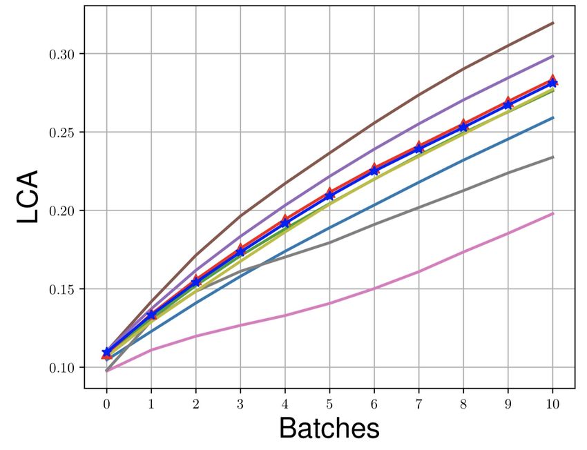
In this paper, we present the first unified view of episodic memory based lifelong learning methods,
including GEM [1] and A-GEM [2], from an optimization’s perspective. Specifically, we cast the
problem of avoiding catastrophic forgetting as an optimization problem with composite objective.
We approximately solve the optimization problem using one-step stochastic gradient descent with
the standard gradient replaced by the proposed Mixed Stochastic Gradient (MEGA). We propose
two different schemes, called MEGA-I and MEGA-II, which can be used in different scenarios. We
show that both GEM [1] and A-GEM [2] are degenerate cases of MEGA-I and MEGA-II which
consistently put the same emphasis on the current task, regardless of how the loss changes over time.
In contrast, based on our derivation, the direction of the proposed MEGA-I and MEGA-II balance
old tasks and the new task in an adaptive manner by considering the performance of the model in the
learning process.
Our contributions are as follows. (1) We present the first unified view of current episodic memory
based lifelong learning methods including GEM [1] and A-GEM [2]. (2) From the presented unified
view, we propose two different schemes, called MEGA-I and MEGA-II, for lifelong learning problems.
(3) We extensively evaluate the proposed schemes on several lifelong learning benchmarks, and
the results show that the proposed MEGA-I and MEGA-II significantly advance the state-of-the-art
performance. We show that the proposed MEGA-I and MEGA-II achieve comparable performance
in the existing setting for lifelong learning [2]. In particular, MEGA-II achieves an average accuracy
of 91.21±0.10% on Permuted MNIST, which is 2% better than the previous state-of-the-art model.
On Split CIFAR, our proposed MEGA-II achieves an average accuracy of 66.12±1.93%, which is
about 5% better than the state-of-the-art method. (4) Finally, we show that the proposed MEGA-II
outperforms MEGA-I when the number of examples per task is limited. We also analyze the reason
for the effectiveness of MEGA-II over MEGA-I in this case.

2   Related Work
Several lifelong learning methods [25, 26] and evaluation protocols [27, 28] are proposed recently.
We categorize the methods into different types based on the methodology,
Regularization based approaches: EWC [4] adopted Fisher information matrix to prevent important
weights for old tasks from changing drastically. In PI [21], the authors introduced intelligent synapses
and endowed each individual synapse with a local measure of “importance” to avoid old memories
from being overwritten. RWALK [22] utilized a KL-divergence based regularization for preserving
knowledge of old tasks. While in MAS [29] the importance measure for each parameter of the
network was computed based on how sensitive the predicted output function is to a change in this
parameter. [30] extended MAS for task-free continual learning. In [31], an approximation of the
Hessian was employed to approximate the posterior after every task. Uncertainties measures were also
used to avoid catastrophic forgetting [32]. [33] proposed methods based on approximate Bayesian
which recursively approximate the posterior of the given data.
Knowledge transfer based methods: In PROG-NN [23], a new “column” with lateral connections
to previous hidden layers was added for each new task. In [34], the authors proposed a method to
leverage unlabeled data in the wild to avoid catastrophic forgetting using knowledge distillation. [35]
proposed orthogonal weights modification (OWM) to enable networks to continually learn different
mapping rules in a context-dependent way.
Episodic memory-based approaches: Augmenting the standard neural network with an external
memory is a widely adopted practice [36, 37, 38]. In episodic memory based lifelong learning
methods, a small reference memory is used for storing information from old tasks. GEM [1] and
A-GEM [2] rotated the current gradient when the angle between the current gradient and the gradient
computed on the reference memory is obtuse. MER [24] is a recently proposed lifelong learning
algorithm which employed a meta-learning training strategy. In [39], a line of methods are proposed
to select important samples to store in the memory in order to reduce memory size. Instead of
storing samples, in [11] the authors proposed Orthogonal Gradient Descent (OGD) which projects
the gradients on the new task onto a subspace in which the projected gradient will not affect the
model’s output on old tasks. [40] proposed conceptor aided backprop which is a variant of the
back-propagation algorithm for avoiding catastrophic forgetting.
Our proposed schemes aim to improve episodic memory based approaches and are most related to [2].
Different from [2], the proposed schemes explicitly consider the performance of the model on old
tasks and the new task in the process of rotating the current gradient. Our proposed schemes are also

                                                   2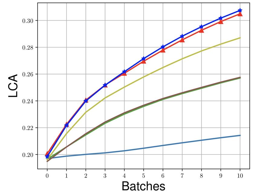
related to several multi-task learning methods [41, 42, 43]. In [41, 42], the authors aimed at achieving
a good balance between different tasks by learning to weigh the loss on each task . In contrast,
our schemes directly leverage loss information in the context of lifelong learning for overcoming
catastrophic forgetting. Compared with [43], instead of using the gradient norm information, our
schemes and [1, 2] focus on rotating the direction of the current gradient. In [44], the authors consider
gradient interference in multi-task learning while we focus on lifelong learning.
3    Lifelong Learning
Lifelong learning (LLL) [1, 2, 4, 23] considers the problem of learning a new task without degrading
performance on old tasks, i.e., to avoid catastrophic forgetting [3, 4]. Suppose there are T tasks
which are characterized by T datasets: {D1 , D2 , .., DT }. Each dataset Dt consists of a list of triplets
(xi , yi , t), where yi is the label of i-th example xi , and t is a task descriptor that indicates which task
the example coming from. Similar to supervised learning, each dataset Dt is split into a training set
Dttr and a test set Dtte .
In the learning protocol introduced in [2], the tasks are separated into DCV = {D1 , D2 , ..., DT CV }
and DEV = {DT CV +1 , DT CV +2 , ..., DT }. DCV is used for cross-validation to search for hyperpa-
rameters. DEV is used for actual training and evaluation. While searching for the hyperparameters,
we can have multiple passes over the examples in DCV , the training is performed on DEV with only
a single pass over the examples [1, 2].
In lifelong learning, a given model f (x; w) is trained sequentially on a series of tasks {DT CV +1 ,
DT CV +2 , ..., DT }. When the model f (x; w) is trained on task Dt , the goal is to predict the labels
of the examples in Dtte by minimizing the empirical loss `t (w) on Dttr in an online fashion without
suffering accuracy drop on {DTteCV +1 , DTteCV +2 , ..., Dtte 1 }.
4    A Unified View of Episodic Memory Based Lifelong Learning
In this section, we provide a unified view for better understanding several episodic memory lifelong
learning approach, including GEM [1] and A-GEM [2]. Due to space constraints, for the details of
GEM and A-GEM, please refer to Appendix A.1.
GEM [1] and A-GEM [2] address the lifelong learning problem by utilizing a small episodic memory
Mk for storing a subset of the examples from task k. The episodic memory is populated by choosing
examples uniformly at random for each task. WhilePtraining on task t, the loss on the episodic
memory Mk can be computed as `ref (wt ; Mk ) = |M1k | (xi ,yi )2Mk `(f (xi ; wt ), yi ), where wt is the
weight of model during the training on task t.
In GEM and A-GEM, the lifelong learning model is trained via mini-batch stochastic gradient descent.
We use wkt to denote the weight when the model is being trained on the k-th mini-batch of task t.
To establish the tradeoff between the performance on old tasks and the t-th task, we consider the
following optimization problem with composite objective in each update step:
                                                       ⇥                                         ⇤
        min ↵1 (wkt )`t (w) + ↵2 (wkt )`ref (w) := E⇠,⇣ ↵1 (wkt )`t (w; ⇠) + ↵2 (wkt )`ref (w; ⇣) , (1)
          w

where w 2 Rd is the parameter of the model, ⇠, ⇣ are random variables with finite support, `t (w) is
the expected training loss of the t-th task, `ref (w) is the expected loss calculated on the data stored in
the episodic memory, ↵1 (w), ↵2 (w) : Rd 7! R+ are real-valued mappings which control the relative
importance of `t (w) and `ref (w) in each mini-batch.
Mathematically, we consider using the following update:
                        t
                       wk+1 = arg min ↵1 (wkt ) · `t (w; ⇠) + ↵2 (wkt ) · `ref (w; ⇣).                       (2)
                                         w

The idea of GEM and A-GEM is to employ first-order methods (e.g., stochastic gradient descent)
to approximately solve the optimization problem (2), where one-step stochastic gradient descent is
performed with the initial point to be wkt :
                    t
                   wk+1      wkt    ⌘ ↵1 (wkt )r`t (wkt ; ⇠kt ) + ↵2 (wkt )r`ref (wkt ; ⇣kt ) ,              (3)
where ⌘ is the learning rate,      ⇠kt  and  ⇣kt     are random variables with finite support,    r`t (wkt ; ⇠kt )
and r`ref (wkt ; ⇣kt ) are unbiased estimators of r`t (wkt ) and r`ref (wkt ) respectively. The quantity
↵1 (wkt )r`t (wkt ; ⇠kt ) + ↵2 (wkt )r`ref (wkt ; ⇣kt ) is referred to as the mixed stochastic gradient.

                                                       3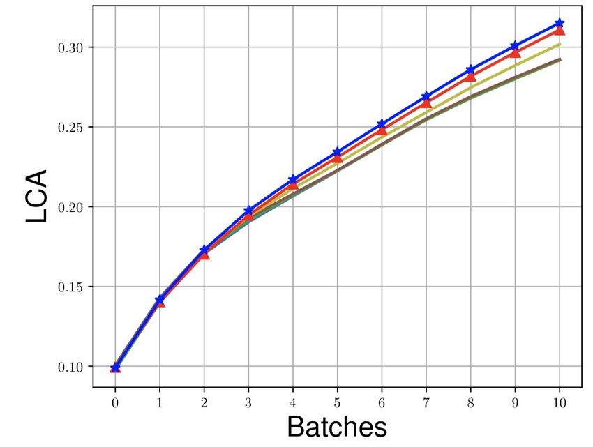
Algorithm 1 The proposed improved schemes for episodic memory based lifelong learning.
1: M {}
2: for t 1 to T do
3: for k 1 to |Dttr | do
4: if M 6= {} then
5: ⇣kt SAMPLE (M )
6: MEGA-I: choose ↵1 and ↵2 based on Equation 6.
7: MEGA-II: choose ↵1 and ↵2 as in Appendix A.3.
8: else
9: Set ↵1 (w) = 1 and ↵2 (w) = 0.
10: end if
11: Update wkS t
using Eq. 3.
12: M M (⇠kt , ykt )
13: Discard the samples added initially if M is full.
14: end for
15: end for
In A-GEM, r`ref (wkt ; ⇠kt ) is the reference gradient computed based on a random subset from the
episodic memory M of all past tasks, where M = [k r`ref (wkt ; ⇣kt )
↵1 (wkt ) = 1, ↵2 (wkt ) = Ihr`ref (wt ;⇣ t ),r`t (wt ;⇠t )i0 ⇥ , (4)
k k k k r`ref (wkt ; ⇣kt )> r`ref (wkt ; ⇣kt )
where Iu is the indicator function, which is 1 if u holds and otherwise 0.
In GEM, there are t 1 reference gradients based on the previous t 1 tasks respectively. In this case,
r`ref (wkt ; ⇣kt ) = [g1 , . . . , gt 1 ] 2 Rd⇥(t 1) and ↵2 (wkt ) 2 Rt 1 , where g1 , . . . , gt 1 are reference
gradients based on M1 , . . . , Mt 1 respectively. In GEM,
↵1 (wkt ) = 1, ↵2 (wkt ) = v⇤ , (5)
where v⇤ is the optimal solution for the quadratic programming problem (11) in Appendix A.1.
As we can see from the formulation (4) and (5), both A-GEM and GEM set ↵1 (w) = 1 in the whole
training process. It means that both A-GEM and GEM always put the same emphasis on the current
task, regardless of how the loss changes over time. During the lifelong learning process, the current
loss and the reference loss are changing dynamically in each mini-batchs, and consistently choosing
↵1 (w) = 1 may not capture a good balance between current loss and the reference loss.
5 Mixed Stochastic Gradient
In this section, we introduce Mixed Stochastic Gradient (MEGA) to address the limitations of
GEM and A-GEM. We adopt the way of A-GEM for computing the reference loss due to the better
performance of A-GEM over GEM. Instead of consistently putting the same emphasis on the current
task, the proposed schemes allow adaptive balancing between current task and old tasks. Specifically,
MEGA-I and MEGA-II utilize the loss information during training which is ignored by GEM and
A-GEM. In Section 5.1, we propose MEGA-I which utilizes loss information to balance the reference
gradient and the current gradient. In Section 5.2, we propose MEGA-II which considers the cosine
similarities between the update direction with the current gradient and the reference gradient.
5.1 MEGA-I
We introduce MEGA-I which is an adaptive loss-based approach to balance the current task and old
tasks by only leveraging loss information. We introduce a pre-defined sensitivity parameter ✏ similar
to [45]. In the update of (3), we set
⇢
↵1 (w) = 1, ↵2 (w) = `ref (w; ⇣)/`t (w; ⇠) if `t (w; ⇠) > ✏
(6)
↵1 (w) = 0, ↵2 (w) = 1 if `t (w; ⇠) ✏,
Intuitively, if `t (w; ⇠) is small, then the model performs well on the current task and MEGA-I focuses
on improving performance on the data stored in the episodic memory. To this end, MEGA-I chooses
4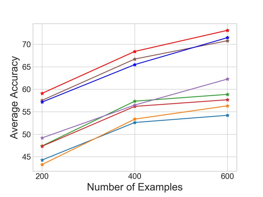
↵1 (w) = 0, ↵2 (w) = 1. Otherwise, when the current loss is larger than ✏, MEGA-I keeps the balance
of the two terms of mixed stochastic gradient according to `t (w; ⇠) and `ref (w; ⇣). Intuitively, if
`t (w; ⇠) is relatively larger than `ref (w; ⇣), then MEGA-I puts less emphasis on the reference gradient
and vice versa.
Compared with GEM and A-GEM update rule in (5) and (4), MEGA-I makes an improvement to
handle the case of overfitting on the current task (i.e., `t (w; ⇠) ✏), and to dynamically change the
relative importance of the current and reference gradient according to the losses on the current task
and previous tasks.
5.2 MEGA-II
The magnitude of MEGA-I’s mixed stochastic gradient depends on the magnitude of the current
gradient and the reference gradient, as well as the losses on the current task and the episodic memory.
Inspired by A-GEM, MEGA-II’s mixed gradient is obtained from a rotation of the current gradient
whose magnitude only depends on the current gradient.
The key idea of the MEGA-II is to first appropriately rotate the stochastic gradient calculated on the
current task (i.e., r`t (wkt ; ⇠kt )) by an angle ✓kt , and then use the rotated vector as the mixed stochastic
gradient to conduct the update (3) in each mini-batch. For simplicity, we omit the subscript k and
superscript t later on unless specified.
We use gmix to denote the desired mixed stochastic gradient which has the same magnitude as
r`t (w; ⇠). Specifically, we look for the mixed stochastic gradient gmix which direction aligns well
with both r`t (w; ⇠) and r`ref (w; ⇣). Similar to MEGA-I, we use the loss-balancing scheme and
desire to maximize
hgmix , r`t (w; ⇠)i hgmix , r`ref (w; ⇣)i
`t (w; ⇠) · + `ref (w; ⇣) · , (7)
kgmix k2 · kr`t (w; ⇠)k2 kgmix k2 · kr`ref (w; ⇣)k2
which is equivalent to find an angle ✓ such that
✓ = arg max `t (w; ⇠) cos( ) + `ref (w; ⇣) cos(✓˜ ). (8)
2[0,⇡]
where ✓˜ 2 [0, ⇡] is the angle between r`t (w; ⇠) and r`ref (w; ⇣), and ⇣ is the ⌘
2 [0, ⇡] angle
k+cos ✓˜
between gmix and r`t (w; ⇠). The closed form of ✓ is ✓ = ⇡
2 ↵, where ↵ = arctan sin ✓˜ and
k = `t (w; ⇠)/`ref (w; ⇣) if `ref (w; ⇣) 6= 0 otherwise k = +1. The detailed derivation of the closed
form of ✓ can be found in Appendix A.2. Here we give some discussions of several special cases of
Eq. (8).
• When `ref (w; ⇣) = 0, then ✓ = 0, and in this case ↵1 (w) = 1, ↵2 (w) = 0 in (3), the mixed
stochastic gradient reduces to r`t (w; ⇠). In the lifelong learning setting, `ref (w; ⇣) = 0
implies that there is almost no catastrophic forgetting, and hence we can update the model
parameters exclusively for the current task by moving in the direction of r`t (w; ⇠).
• When `t (w; ⇠) = 0, then ✓ = ✓, ˜ and in this case ↵1 (w) = 0, ↵2 (w) =
kr`t (w; ⇠)k2 /kr`ref (w; ⇣)k2 , provided that kr`ref (w; ⇣)k2 6= 0 (define 0/0=0). In this
case, the direction of the mixed stochastic gradient is the same as the stochastic gradient
calculated on the data in the episodic memory (i.e., `ref (w; ⇣)). In the lifelong learning
setting, this update can help improve the performance on old tasks, i.e., avoid catastrophic
forgetting.
After we find the desired angle ✓, we can calculate ↵1 (w) and ↵2 (w) in Eq. (3), as shown in
Appendix A.3. It is worth noting that different from GEM and A-GEM which always set ↵1 (w) = 1,
the proposed MEGA-I and MEGA-II adaptively adjust ↵1 and ↵2 based on performance of the
model on the current task and the episodic memory. Please see Algorithm 1 for the summary of the
algorithm.
6 Experiments
6.1 Experimental Settings and Evaluation Protocol
We conduct experiments on commonly used lifelong learning bencnmarks: Permutated MNIST [4],
Split CIFAR [21], Split CUB [2], Split AWA [2]. The details of the datasets can be found in
50.70 0.30
1.00 1.0 0.38 1.0
0.50 0.28
0.65 0.25 0.35
0.90
0.40 0.8 0.8
0.26
0.60 0.33
0.80 0.20
0.30 0.6 0.55 0.30 0.6
0.24
0.70 0.15
0.50 0.28
0.20 0.4 0.4
0.60 0.22 0.10
0.45 0.25
0.50 0.10 0.2 0.2
0.20 0.05
0.23
0.40
0.00 0.0 0.00 0.20 0.0
FT ( ) LCA10 ( ) Time( ) Mem( ) AT ( ) FT ( ) LCA10 ( ) Time( ) Mem( )
(a) Permuted MNIST (b) Split CIFAR
0.32
1.0
0.80 0.150 0.30
0.32 0.55 0.10
0.30
0.125 0.8 0.25
0.75 0.50
0.08 0.28
0.100 0.31
0.70 0.20
0.6 0.45
0.075 0.26
0.06
0.65 0.30 0.40 0.15
0.4
0.050 0.24
0.35 0.04 0.10
0.60
0.025 0.29
0.2 0.22
0.30 0.05
0.55
0.02
0.000
0.28 0.20
0.0 0.00
AT ( ) FT ( ) LCA10 ( ) Time( ) Mem( ) AT ( ) FT ( ) LCA10 ( ) Time( ) Mem( )
(c) Split CUB (d) Split AWA
Figure 1: Performance of lifelong learning models across different measures on Permuted MNIST,
Split CIFAR, Split CUB and Split AWA.
Appendix A.4. We compare MEGA-I and MEGA-II with several baselines, including VAN [2],
MULTI-TASK [2], EWC [4], PI [21], MAS [29], RWALK [22], ICARL [46], PROG-NN [23], MER
[24], GEM [1] and A-GEM [2]. In particular, in VAN [2], a single network is trained continuously on
a sequence of tasks in a standard supervised learning manner. In MULTI-TASK [2], a single network
is trained on the shuffled data from all the tasks with a single pass.
To be consistent with the previous works [1, 2], for Permuted MNIST we adopt a standard fully-
connected network with two hidden layers. Each layer has 256 units with ReLU activation. For Split
CIFAR we use a reduced ResNet18. For Split CUB and Split AWA, we use a standard ResNet18
[47]. We use Average Accuracy (AT ), Forgetting Measure (FT ) and Learning Curve Area (LCA)
[1, 2] for evaluating the performance of lifelong learning algorithms. AT is the average test accuracy
and FT is the degree of accuracy drop on old tasks after the model is trained on all the T tasks. LCA
is used to assess the learning speed of different lifelong learning algorithms. Please see Appendix
A.5 for the definitions of different metrics.
To be consistent with [2], for episodic memory based approaches, the episodic memory size for
each task is 250, 65, 50, and 100, and the batch size for computing the gradients on the episodic
memory (if needed) is 256, 1300, 128 and 128 for MNIST, CIFAR, CUB and AWA, respectively. To
fill the episodic memory, the examples are chosen uniformly at random for each task as in [2]. For
each dataset, 17 tasks are used for training and 3 tasks are used for hyperparameter search. For the
baselines, we use the best hyperparameters found by [2]. For the detailed hyperparameters, please see
Appendix G of [2]. For MER [24], we reuse the best hyperparameters found in [24]. In MEGA-I, the
✏ is chosen from {10 5:1: 1 } via the 3 validation tasks. For MEGA-II, we reuse the hyperparameters
from A-GEM [2]. All the experiments are done on 8 NVIDIA TITAN RTX GPUs. The code can be
found in the supplementary material.
6.2 Results
6.2.1 MEGA VS Baselines
In Fig. 1 we show the results across different measures on all the benchmark datasets. We have the
following observations. First, MEGA-I and MEGA-II outperform all baselines across the benchmarks,
except that PROG-NN achieves a slightly higher accuracy on Permuted MNIST. As we can see
from the memory comparison, PROG-NN is very memory inefficient since it allocates a new network
for each task, thus the number of parameters grows super-linearly with the number of tasks. This
becomes problematic when large networks are being used. For example, PROG-NN runs out of
memory on Split CUB and Split AWA which prevents it from scaling up to real-life problems. On
other datasets, MEGA-I and MEGA-II consistently perform better than all the baselines. From
6(a) Permuted MNIST (b) Split CIFAR
(c) Split CUB (d) Split AWA
Figure 2: Evolution of average accuracy during the lifelong learning process.
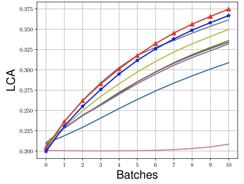
(a) Permuted MNIST (b) Split CIFAR (c) Split CUB (d) Split AWA
Figure 3: LCA of first ten mini-batches on different datasets.
Fig. 2 we can see that on Split CUB, MEGA-I and MEGA-II even surpass the multi-task baseline
which is previously believed as an upper bound performance of lifelong learning algorithms [2].
Second, MEGA-I and MEGA-II achieve the lowest Forgetting Measure across all the datasets which
indicates their ability to overcome catastrophic forgetting. Third, MEGA-I and MEGA-II also obtain
a high LCA across all the datasets which shows that MEGA-I and MEGA-II also learn quickly. The
evolution of LCA in the first ten mini-batches across all the datasets is shown in Fig. 3. Last, we
can observe that MEGA-I and MEGA-II achieve similar results in Fig. 1. For detailed results, please
refer to Table 2 and Table 3 in Appendix A.6.
In Fig. 2 we show the evolution of average accuracy during the lifelong learning process. As more
tasks are added, while the average accuracy of the baselines generally drops due to catastrophic
forgetting, MEGA-I and MEGA-II can maintain and even improve their performance. In the next
section, we will show that MEGA-II outperforms MEGA-I when the number of examples is limited
per task.
6.2.2 MEGA-II Outperforms Other Baselines and MEGA-I When the Number of Examples
is Limited
Inspired by few-shot learning [48, 49, 50, 51], in this section we consider a more challenging setting
for lifelong learning where each task only has a limited number of examples.
We construct 20 tasks with X number of examples per task, where X = 200, 400 and 600. The way
to generate the tasks is the same as in Permuted MNIST, that is, a fixed random permutation of
input pixels is applied to all the examples for a particular task. The running time is measured on one
NVIDIA TITAN RTX GPU. The results of average accuracy are shown in Fig. 4(a). We can see that
MEGA-II outperforms all the baseline and MEGA-I when the number of examples is limited. In
Fig. 4(b), we show the execution time for each method, the proposed MEGA-I and MEGA-II are
7(a) (b)
Figure 4: The average accuracy and execution time when the number of examples is limited.
computational efficient compared with other methods. Compared with MER [24] which achieves
similar results to MEGA-I and MEGA-II, MEGA-I and MEGA-II is much more time efficient since
it does not rely on the meta-learning procedure.
We analyze the reason why MEGA-II outperforms MEGA-I when the number of examples is small.
In this case, it is difficult to learn well on the current task, so the magnitude of the current loss and
the current gradient’s norm are both large. MEGA-I directly balances the reference gradient and the
current gradient, and the mixed stochastic gradient is dominated by the current gradient and it suffers
from catastrophic forgetting. In contrast, MEGA-II balances the cosine similarity between gradients.
Even if the norm of the current gradient is large, MEGA-II still allows adequate rotation of the
direction of the current gradient to be closer to that of the reference gradient to alleviate catastrophic
forgetting. We validate our claims by detailed analysis, which can be found in Appendix A.7.
6.2.3 Ablation Studies
In this section, we include detailed ablation studies to analyze the reason why the proposed schemes
can improve current episodic memory based lifelong learning methods. For MEGA-I, we consider
the setting that both ↵1 (w) = 1 and ↵2 (w) = 1 during the training process. This ablation study
is to show the effectiveness of the adaptive loss balancing scheme. For MEGA-II, we consider the
setting that `t = `ref in Eq. 7 to verify the effectiveness of the proposed gradient rotation scheme over
A-GEM. The experimental settings are the same as Section 6.1. The results are shown in Table 1.
Table 1: Comparison of MEGA-I, MEGA-I (↵1 (w) = 1, ↵2 (w) = 1), MEGA-II, MEGA-II (`t =
`ref ) and A-GEM.
Method Permuted MNIST Split CIFAR Split CUB Split AWA
AT (%) AT (%) AT (%) AT (%)
MEGA-I 91.10 ± 0.08 66.10 ± 1.67 79.67 ± 2.15 54.82 ± 4.97
MEGA-I (↵1 (w) =
90.66 ± 0.09 64.65 ± 1.98 79.44 ± 2.98 53.60 ± 5.21
1, ↵2 (w) = 1)
MEGA-II 91.21 ± 0.10 66.12 ± 1.93 80.58 ± 1.94 54.28 ± 4.84
MEGA-II (`t = `ref ) 91.15 ± 0.12 58.04 ± 1.89 68.60 ± 1.98 47.95 ± 4.54
A-GEM 89.32 ± 0.46 61.28 ± 1.88 61.82 ± 3.72 44.95 ± 2.97
In Table 1, we observe that MEGA-I achieves higher average accuracy than MEGA-I (↵1 (w) =
1, ↵2 (w) = 1) by considering an adaptive loss balancing scheme. We also see that except on Split
CIFAR, MEGA-II (`t = `ref ) outperforms A-GEM on all the datasets. This demonstrates the benefits
of the proposed approach for rotating the current gradient. By considering the loss information
as in MEGA-II, we further improve the results on all the datasets. This shows that both of the
components (the rotation of the current gradient and loss balancing) contribute to the improvements
of the proposed schemes.
7 Conclusion
In this paper, we cast the lifelong learning problem as an optimization problem with composite
objective, which provides a unified view to cover current episodic memory based lifelong learning
algorithms. Based on the unified view, we propose two improved schemes called MEGA-I and
8MEGA-II. Extensive experimental results show that the proposed MEGA-I and MEGA-II achieve
superior performance, significantly advancing the state-of-the-art on several standard benchmarks.
9Acknowledgment
This work was supported in part by CRISP, one of six centers in JUMP, an SRC program sponsored
by DARPA. This work is also supported by NSF CHASE-CI #1730158, NSF FET #1911095, NSF
CC* NPEO #1826967, NSF #1933212, NSF CAREER Award #1844403. The paper was also funded
in part by SRC AIHW grants.
Broader Impact
In this paper, researchers introduce a unified view on current episodic memory based lifelong learning
methods and propose two improved schemes: MEGA-I and MEGA-II. The proposed schemes
demonstrate superior performance and advance the state-of-the-art on several lifelong learning
benchmarks.
The unified view embodies existing episodic memory based lifelong learning methods in the same
general framework. The proposed MEGA-I and MEGA-II significantly improve existing episodic
memory based lifelong learning such as GEM [1] and A-GEM [2]. The proposed schemes enable
machine learning models to acquire the ability to learn tasks sequentially without catastrophic
forgetting. Machine learning models with continual learning capability can be applied in image
classification [1] and natural language processing [52].
The proposed lifelong learning algorithms can be applied in several real-world applications such
as on-line advertisement, fraud detection, climate change monitoring, recommendation systems,
industrial manufacturing and so on. In all these applications, the data are arriving sequentially and
the data distribution may change over time. For example, in recommendation systems, the users’
preferences may vary due to their aging, personal financial status or health condition. The machine
learning models without continual learning capability may not capture such dynamics. The proposed
lifelong learning schemes are able to address this issue.
The related applications have a broad range of societal implications: the use of lifelong recommenda-
tion systems can bring several benefits such as reducing the cost of model retraining and providing
better user experience. However, such systems may have the concerns of data privacy. Lifelong
recommendation systems can increase customer satisfaction. In the mean time, this system needs to
store part of user data which may compromise user’s privacy.
Our proposed lifelong learning schemes also are closely related to other machine learning research
areas, including multi-task learning, transfer learning, federated learning, few-shot learning and so
on. In transfer learning, when the source domain and the target domain are different, it is crucial to
develop techniques that can reduce the negative transfer between the domains during the fine-tuning
process. We expect that our proposed approaches can be leveraged to resolve the issue of negative
transfer.
We encourage researchers to further investigate the merits and shortcomings of our proposed methods.
In particular, we recommend researchers and policymakers to look into lifelong learning systems
without storing examples from past tasks. Such systems do not jeopardize users’ privacy and can be
deployed in critical scenarios such as financial applications.
10References
[1] David Lopez-Paz et al. Gradient episodic memory for continual learning. In Advances in Neural
Information Processing Systems, pages 6467–6476, 2017.
[2] Arslan Chaudhry, Marc’Aurelio Ranzato, Marcus Rohrbach, and Mohamed Elhoseiny. Efficient
lifelong learning with a-gem. arXiv preprint arXiv:1812.00420, 2018.
[3] Robert M French. Catastrophic forgetting in connectionist networks. Trends in cognitive
sciences, 3(4):128–135, 1999.
[4] James Kirkpatrick, Razvan Pascanu, Neil Rabinowitz, Joel Veness, Guillaume Desjardins,
Andrei A Rusu, Kieran Milan, John Quan, Tiago Ramalho, Agnieszka Grabska-Barwinska, et al.
Overcoming catastrophic forgetting in neural networks. Proceedings of the national academy of
sciences, 114(13):3521–3526, 2017.
[5] Roger Ratcliff. Connectionist models of recognition memory: constraints imposed by learning
and forgetting functions. Psychological review, 97(2):285, 1990.
[6] Ian Goodfellow, Yoshua Bengio, Aaron Courville, and Yoshua Bengio. Deep learning, volume 1.
MIT Press, 2016.
[7] Anthony Robins. Catastrophic forgetting, rehearsal and pseudorehearsal. Connection Science,
7(2):123–146, 1995.
[8] Xilai Li, Yingbo Zhou, Tianfu Wu, Richard Socher, and Caiming Xiong. Learn to grow: A
continual structure learning framework for overcoming catastrophic forgetting. arXiv preprint
arXiv:1904.00310, 2019.
[9] Cuong V Nguyen, Alessandro Achille, Michael Lam, Tal Hassner, Vijay Mahadevan, and
Stefano Soatto. Toward understanding catastrophic forgetting in continual learning. arXiv
preprint arXiv:1908.01091, 2019.
[10] Cuong V Nguyen, Yingzhen Li, Thang D Bui, and Richard E Turner. Variational continual
learning. arXiv preprint arXiv:1710.10628, 2017.
[11] Mehrdad Farajtabar, Navid Azizan, Alex Mott, and Ang Li. Orthogonal gradient descent for
continual learning. arXiv preprint arXiv:1910.07104, 2019.
[12] David Rolnick, Arun Ahuja, Jonathan Schwarz, Timothy Lillicrap, and Gregory Wayne. Expe-
rience replay for continual learning. In Advances in Neural Information Processing Systems,
pages 348–358, 2019.
[13] Michalis K Titsias, Jonathan Schwarz, Alexander G de G Matthews, Razvan Pascanu, and
Yee Whye Teh. Functional regularisation for continual learning using gaussian processes. arXiv
preprint arXiv:1901.11356, 2019.
[14] Tameem Adel, Han Zhao, and Richard E Turner. Continual learning with adaptive weights
(claw). arXiv preprint arXiv:1911.09514, 2019.
[15] German I Parisi, Ronald Kemker, Jose L Part, Christopher Kanan, and Stefan Wermter. Continual
lifelong learning with neural networks: A review. Neural Networks, 2019.
[16] Sebastian Thrun and Tom M Mitchell. Lifelong robot learning. Robotics and autonomous
systems, 15(1-2):25–46, 1995.
[17] Jaehong Yoon, Eunho Yang, Jeongtae Lee, and Sung Ju Hwang. Lifelong learning with
dynamically expandable networks. arXiv preprint arXiv:1708.01547, 2017.
[18] Sang-Woo Lee, Jin-Hwa Kim, Jaehyun Jun, Jung-Woo Ha, and Byoung-Tak Zhang. Overcoming
catastrophic forgetting by incremental moment matching. In Advances in neural information
processing systems, pages 4652–4662, 2017.
[19] Mariya Toneva, Alessandro Sordoni, Remi Tachet des Combes, Adam Trischler, Yoshua Bengio,
and Geoffrey J Gordon. An empirical study of example forgetting during deep neural network
learning. arXiv preprint arXiv:1812.05159, 2018.
[20] Hanul Shin, Jung Kwon Lee, Jaehong Kim, and Jiwon Kim. Continual learning with deep
generative replay. In Advances in Neural Information Processing Systems, pages 2990–2999,
2017.
11[21] Friedemann Zenke, Ben Poole, and Surya Ganguli. Continual learning through synaptic
intelligence. In Proceedings of the 34th International Conference on Machine Learning-Volume
70, pages 3987–3995. JMLR. org, 2017.
[22] Arslan Chaudhry, Puneet K Dokania, Thalaiyasingam Ajanthan, and Philip HS Torr. Riemannian
walk for incremental learning: Understanding forgetting and intransigence. In Proceedings of
the European Conference on Computer Vision (ECCV), pages 532–547, 2018.
[23] Andrei A Rusu, Neil C Rabinowitz, Guillaume Desjardins, Hubert Soyer, James Kirkpatrick,
Koray Kavukcuoglu, Razvan Pascanu, and Raia Hadsell. Progressive neural networks. arXiv
preprint arXiv:1606.04671, 2016.
[24] Matthew Riemer, Ignacio Cases, Robert Ajemian, Miao Liu, Irina Rish, Yuhai Tu, and Ger-
ald Tesauro. Learning to learn without forgetting by maximizing transfer and minimizing
interference. arXiv preprint arXiv:1810.11910, 2018.
[25] Matthias De Lange, Rahaf Aljundi, Marc Masana, Sarah Parisot, Xu Jia, Ales Leonardis,
Gregory Slabaugh, and Tinne Tuytelaars. Continual learning: A comparative study on how to
defy forgetting in classification tasks. arXiv preprint arXiv:1909.08383, 2019.
[26] Ronald Kemker, Marc McClure, Angelina Abitino, Tyler L Hayes, and Christopher Kanan.
Measuring catastrophic forgetting in neural networks. In Thirty-second AAAI conference on
artificial intelligence, 2018.
[27] Sebastian Farquhar and Yarin Gal. Towards robust evaluations of continual learning. arXiv
preprint arXiv:1805.09733, 2018.
[28] Tyler L Hayes, Ronald Kemker, Nathan D Cahill, and Christopher Kanan. New metrics and
experimental paradigms for continual learning. In Proceedings of the IEEE Conference on
Computer Vision and Pattern Recognition Workshops, pages 2031–2034, 2018.
[29] Rahaf Aljundi, Francesca Babiloni, Mohamed Elhoseiny, Marcus Rohrbach, and Tinne Tuyte-
laars. Memory aware synapses: Learning what (not) to forget. In Proceedings of the European
Conference on Computer Vision (ECCV), pages 139–154, 2018.
[30] Rahaf Aljundi, Klaas Kelchtermans, and Tinne Tuytelaars. Task-free continual learning. In
Proceedings of the IEEE Conference on Computer Vision and Pattern Recognition, pages
11254–11263, 2019.
[31] Hippolyt Ritter, Aleksandar Botev, and David Barber. Online structured laplace approximations
for overcoming catastrophic forgetting. In Advances in Neural Information Processing Systems,
pages 3738–3748, 2018.
[32] Sayna Ebrahimi, Mohamed Elhoseiny, Trevor Darrell, and Marcus Rohrbach. Uncertainty-
guided continual learning with bayesian neural networks. arXiv preprint arXiv:1906.02425,
2019.
[33] Sebastian Farquhar and Yarin Gal. A unifying bayesian view of continual learning. arXiv
preprint arXiv:1902.06494, 2019.
[34] Kibok Lee, Kimin Lee, Jinwoo Shin, and Honglak Lee. Overcoming catastrophic forgetting
with unlabeled data in the wild. In Proceedings of the IEEE International Conference on
Computer Vision, pages 312–321, 2019.
[35] Guanxiong Zeng, Yang Chen, Bo Cui, and Shan Yu. Continual learning of context-dependent
processing in neural networks. Nature Machine Intelligence, 1(8):364–372, 2019.
[36] Jason Weston, Sumit Chopra, and Antoine Bordes. Memory networks. arXiv preprint
arXiv:1410.3916, 2014.
[37] Alexander Pritzel, Benigno Uria, Sriram Srinivasan, Adria Puigdomenech, Oriol Vinyals, Demis
Hassabis, Daan Wierstra, and Charles Blundell. Neural episodic control. arXiv preprint
arXiv:1703.01988, 2017.
[38] Adam Santoro, Sergey Bartunov, Matthew Botvinick, Daan Wierstra, and Timothy Lillicrap.
One-shot learning with memory-augmented neural networks. arXiv preprint arXiv:1605.06065,
2016.
[39] Rahaf Aljundi, Min Lin, Baptiste Goujaud, and Yoshua Bengio. Gradient based sample selection
for online continual learning. In Advances in Neural Information Processing Systems, pages
11816–11825, 2019.
12[40] Xu He and Herbert Jaeger. Overcoming catastrophic interference using conceptor-aided back-
propagation. In International Conference on Learning Representations, 2018.
[41] Ozan Sener and Vladlen Koltun. Multi-task learning as multi-objective optimization. In
Advances in Neural Information Processing Systems, pages 527–538, 2018.
[42] Alex Kendall, Yarin Gal, and Roberto Cipolla. Multi-task learning using uncertainty to weigh
losses for scene geometry and semantics. In Proceedings of the IEEE Conference on Computer
Vision and Pattern Recognition, pages 7482–7491, 2018.
[43] Zhao Chen, Vijay Badrinarayanan, Chen-Yu Lee, and Andrew Rabinovich. Gradnorm: Gra-
dient normalization for adaptive loss balancing in deep multitask networks. arXiv preprint
arXiv:1711.02257, 2017.
[44] Tianhe Yu, Saurabh Kumar, Abhishek Gupta, Sergey Levine, Karol Hausman, and Chelsea Finn.
Gradient surgery for multi-task learning. arXiv preprint arXiv:2001.06782, 2020.
[45] Koby Crammer, Ofer Dekel, Joseph Keshet, Shai Shalev-Shwartz, and Yoram Singer. Online
passive-aggressive algorithms. Journal of Machine Learning Research, 7(Mar):551–585, 2006.
[46] Sylvestre-Alvise Rebuffi, Alexander Kolesnikov, Georg Sperl, and Christoph H Lampert. icarl:
Incremental classifier and representation learning. In Proceedings of the IEEE conference on
Computer Vision and Pattern Recognition, pages 2001–2010, 2017.
[47] Kaiming He, Xiangyu Zhang, Shaoqing Ren, and Jian Sun. Deep residual learning for image
recognition. In Proceedings of the IEEE conference on computer vision and pattern recognition,
pages 770–778, 2016.
[48] Jake Snell, Kevin Swersky, and Richard Zemel. Prototypical networks for few-shot learning. In
Advances in neural information processing systems, pages 4077–4087, 2017.
[49] Oriol Vinyals, Charles Blundell, Timothy Lillicrap, Daan Wierstra, et al. Matching networks
for one shot learning. In Advances in neural information processing systems, pages 3630–3638,
2016.
[50] Chelsea Finn, Pieter Abbeel, and Sergey Levine. Model-agnostic meta-learning for fast adap-
tation of deep networks. In Proceedings of the 34th International Conference on Machine
Learning-Volume 70, pages 1126–1135. JMLR. org, 2017.
[51] Yunhui Guo, Noel CF Codella, Leonid Karlinsky, John R Smith, Tajana Rosing, and Rogerio
Feris. A new benchmark for evaluation of cross-domain few-shot learning. arXiv preprint
arXiv:1912.07200, 2019.
[52] Cyprien de Masson d’Autume, Sebastian Ruder, Lingpeng Kong, and Dani Yogatama. Episodic
memory in lifelong language learning. In Advances in Neural Information Processing Systems,
pages 13122–13131, 2019.
[53] Yann LeCun, Corinna Cortes, and Christopher JC Burges. The mnist database. URL http://yann.
lecun. com/exdb/mnist, 1998.
[54] Alex Krizhevsky et al. Learning multiple layers of features from tiny images. Technical report,
Citeseer, 2009.
[55] Catherine Wah, Steve Branson, Peter Welinder, Pietro Perona, and Serge Belongie. The
caltech-ucsd birds-200-2011 dataset. 2011.
[56] Christoph H Lampert, Hannes Nickisch, and Stefan Harmeling. Learning to detect unseen
object classes by between-class attribute transfer. In 2009 IEEE Conference on Computer Vision
and Pattern Recognition, pages 951–958. IEEE, 2009.
13You can also read