Leveraging Deep Learning for Visual Odometry Using Optical Flow
←
→
Page content transcription
If your browser does not render page correctly, please read the page content below

sensors
Communication
Leveraging Deep Learning for Visual Odometry Using
Optical Flow
Tejas Pandey *, Dexmont Pena, Jonathan Byrne                         and David Moloney

                                           Intel Research & Development, W23 CX68 Leixlip, Ireland; dexmont.pena@intel.com (D.P.);
                                           jonathan.byrne@intel.com (J.B.); david.moloney@intel.com (D.M.)
                                           * Correspondence: tejas.pandey@intel.com

                                           Abstract: In this paper, we study deep learning approaches for monocular visual odometry (VO).
                                           Deep learning solutions have shown to be effective in VO applications, replacing the need for highly
                                           engineered steps, such as feature extraction and outlier rejection in a traditional pipeline. We propose
                                           a new architecture combining ego-motion estimation and sequence-based learning using deep neural
                                           networks. We estimate camera motion from optical flow using Convolutional Neural Networks
                                           (CNNs) and model the motion dynamics using Recurrent Neural Networks (RNNs). The network
                                           outputs the relative 6-DOF camera poses for a sequence, and implicitly learns the absolute scale
                                           without the need for camera intrinsics. The entire trajectory is then integrated without any post-
                                           calibration. We evaluate the proposed method on the KITTI dataset and compare it with traditional
                                           and other deep learning approaches in the literature.

                                           Keywords: visual odometry; ego-motion estimation; deep learning

                                           1. Introduction

                                         Visual odometry [1] is the challenging task of camera pose estimation and robot
                                           localization based only on visual feedback. It represents one of the fundamental problems
Citation: Pandey, T.; Pena, D.; Byrne,
                                           of computer vision, and forms an integral part of Simultaneous Localization And Mapping
J.; Moloney, D. Leveraging Deep
                                           (SLAM) and robot kinematics. It is a long-standing challenge in the field, and is being
Learning for Visual Odometry Using
Optical Flow. Sensors 2021, 21, 1313.
                                           worked on for several decades [2,3].
https://doi.org/10.3390/s21041313
                                                Visual odometry forms an integral component for autonomous agents. A self-driving
                                           agent is responsible for being aware of the environment and other moving objects in the
Academic Editor: Steve Vanlanduit          scene, as well as its own relative movements. Given a sequence of frames, the agent
Received: 8 January 2021                   needs to keep track of the relative inter-frame motion, as well as positioning on a global
Accepted: 9 February 2021                  scale. Marginal errors called “drift” are introduced in the relative motion prediction. They
Published: 12 February 2021                accumulate over the length of a path and propagate throughout the global trajectory,
                                           leading to significant errors.
Publisher’s Note: MDPI stays neu-               Classical visual odometry is dominated by stereoscopic and RGB-D cameras where
tral with regard to jurisdictional clai-   information such as scale, which gets lost during projection mapping, can be recovered to
ms in published maps and institutio-       reduce the drift [4–7]. Others rely on sensor fusion, where data from multiple sensors, such
nal affiliations.                          as LIDAR, IMU, and GPS are fused to come up with more reliable and robust solutions [8,9].
                                           Recently, there has been an increased interest in problems regarding ego-motion with the
                                           rise of autonomous agents navigating in unfamiliar dynamic environments, such as self-
Copyright: © 2021 by the authors. Li-
                                           driving cars and UAV drones, leading to a demand for cheap and reliable commodity
censee MDPI, Basel, Switzerland.
                                           solutions. Integrating multiple cameras with different sensors requires not only space and
This article is an open access article
                                           expensive hardware, but also sufficient processing power and energy. Even stereoscopic
distributed under the terms and con-       cameras are constrained if the robot is too small and cameras are too close. Monocular
ditions of the Creative Commons At-        visual odometry has the advantage of using only a single camera; however, it is significantly
tribution (CC BY) license (https://        more challenging due to the number of ambiguities involved. These challenges include loss
creativecommons.org/licenses/by/           of scale, dynamic environments, inconsistent changes in illumination, and occlusion [10].
4.0/).                                     Traditional approaches can be divided into two categories: direct, and feature-based.

Sensors 2021, 21, 1313. https://doi.org/10.3390/s21041313                                                   https://www.mdpi.com/journal/sensors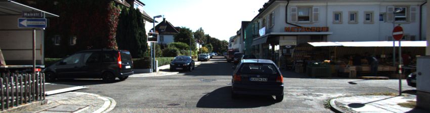
Sensors 2021, 21, 1313                                                                                                2 of 13

                              Feature-based methods [11–13] extract geometrically consistent features [14] and track
                         them across subsequent frames. The camera motion is estimated by minimizing re-
                         projection errors between feature pairs. Though feature-based methods are robust to
                         noise, they fail to work in sparse, textureless environments where the algorithm is unable
                         to generate suitable features.
                              Direct methods [15] track the intensity of pixels and estimate camera motion by mini-
                         mizing photometric errors. They are more robust in environments lacking visual features,
                         but are susceptible to sudden changes between subsequent frames.
                              In computer vision, deep learning-based approaches have outperformed traditional
                         methods in tasks such as object classification and detection [16–18]. However, these
                         approaches are unsuitable for geometric tasks, as they were designed to be transla-
                         tion/orientation invariant, rather than equivariant. They lose track of spatial relationships
                         and ignore physical features such as size, velocity, and orientation. Different adaptions
                         were designed to overcome this problem [19,20].
                              In this paper, we first study the problem of visual odometry using deep neural
                         networks. We search for deep learning approaches to overcome the limitations present
                         in direct and feature-based methods. Deep neural networks learn feature representations
                         in higher dimensions and can replace the engineering effort required in integrating and
                         fine-tuning individual components [1,21].
                              We then propose a pipeline using CNNs that takes optical flow as input and directly
                         estimates a relative 6-DOF camera pose. We augment the network with RNNs, as repre-
                         sented in Figure 1, to implicitly model relationships between subsequent frames in higher
                         dimensions.
                              The rest of the paper goes as follows—Section 2 reviews related work and Section 3
                         comprises our proposed model, followed by experimental results in Section 4 and the
                         conclusion in Section 5.

                         Figure 1. Overview of our approach: Optical flow is passed on to CNNs, extracting relevant features,
                         which are in turn passed on to the RNNs.

                         2. Related Work
                              Monocular visual odometry is the task of tracking the flow of information from a
                         single camera and predicting the path undertaken by it. Traditional methods [12,22,23] are
                         solely insufficient and have to rely on external parameters to account for the ambiguities
                         involved, such as scale, whereas deep learning approaches [24,25] are self-sufficient and
                         show improved results compared to older traditional methods.
                              Recent deep learning approaches [26,27] propose taking a pre-trained FlownetS [28]
                         and re-purposing it to predict relative poses. The FlownetS architecture, given two RGB
                         images, uses a single network for feature extraction and matching to estimate optical flow.
                         The hypothesis is that the features learned for capturing the relationship between frames
Sensors 2021, 21, 1313                                                                                            3 of 13

                         for estimating optical flow should also be suitable for the task of predicting the relative
                         pose between them.
                              Another approach is to directly use optical flow as input [26,29] and regress the relative
                         pose based on learned priors. The advantage here is that it also allows us to decouple the
                         problem of visual odomtery into feature extraction and motion estimation.

                         2.1. Sequence-Based Modelling
                              Wang et al. [24] were the first ones to propose a sequence-based model. They argued
                         that CNNs were not sufficient to model the visual odometry pipeline (VO). While CNNs are
                         useful for learning visual features, they cannot capture motion dynamics. They proposed
                         using LSTMs to capture the temporal relationship between frames. However, LSTMs
                         are not suitable for working with high-dimensional data, such as high-resolution images.
                         Thus, the FlownetS architecture is augmented with LSTMs to model the entire VO pipeline.
                         Feature representations extracted from CNNs are passed onto LSTMs, which output pose
                         estimates at every timestep.
                              Parisotto et al. [27] countered that while LSTMs can model relationships between
                         frames, they cannot influence past outputs, and proposed an attention-based, neural global-
                         bundle adjustment network. The output features from FlownetS are passed onto the
                         global-adjustment network, which uses temporal convolutions to account for drift over
                         long trajectories. Subsequently predicted trajectories can be refined by recursively passing
                         the outputs back to the global-adjustment network.
                              Jiao et al. [25] proposed an iterative update to [24] using bi-directional LSTMs, and
                         outperformed [24] on the KITTI dataset. Bi-directional LSTMs model relationships for
                         both forward and backward sequences. LSTMs learn to model the conditional probability
                         between poses. A bi-directional LSTM would open up the probable space by learning from
                         future sequences as well.

                         2.2. Optical Flow-Based Visual Odometry
                               Costante and Ciarfuglia [30] argued that deep learning approaches involved not only
                         learning visual cues, but camera intrinsics as well. They recommended decoupling the
                         learning of visual and motion features for better generalization. Rather than use a single
                         network for feature extraction and motion estimation, they proposed an auto-encoder to
                         capture an embedding of the optical flow and thereby predict the relative pose based off
                         of it. They formed a multi-objective loss function to minimize the error in reconstruction
                         of optical flow and camera pose estimation, thus ensuring the captured embedding was
                         suitable for motion estimation. They were able to outperform traditional monocular
                         approaches [13,31]. However, a multi-objective function can hinder the performance of
                         motion prediction where the network can struggle to balance the loss of optical flow
                         reconstruction and pose estimation. Moreover, the two tasks may not share favourable
                         features, thus reducing the accuracy of both reconstruction and pose prediction [32].
                               Costante et al. [29] used optical flow as an input to estimate the camera pose. In
                         order to retain the spatial relationship, they proposed splitting the input optical flow
                         into quadrants and passing individual quadrants into a combination of 5 different neural
                         networks—one for every quadrant, and one for the entire optical flow. Different regions
                         add value for specific directions, and thus, splitting the optical flow into quadrants allowed
                         us to preserve such information from shared parameters. Outputs of all networks were
                         concatenated in order to regress the relative translation and rotation parameters. They
                         were able to outperform traditional monocular methods as well. However, their approach
                         required five networks, which is computationally expensive and memory-intensive.
                               Muller and Savakis [26] proposed using the same architecture as FlownetS while pass-
                         ing 2D optical flow vectors as input, rather than a six-channel concatenated RGB pair. They
                         used the same hyper-parameters due to FlownetS’ success on RGB images and performed
                         pose estimation using a single network, passing optical flow vectors as input. However, a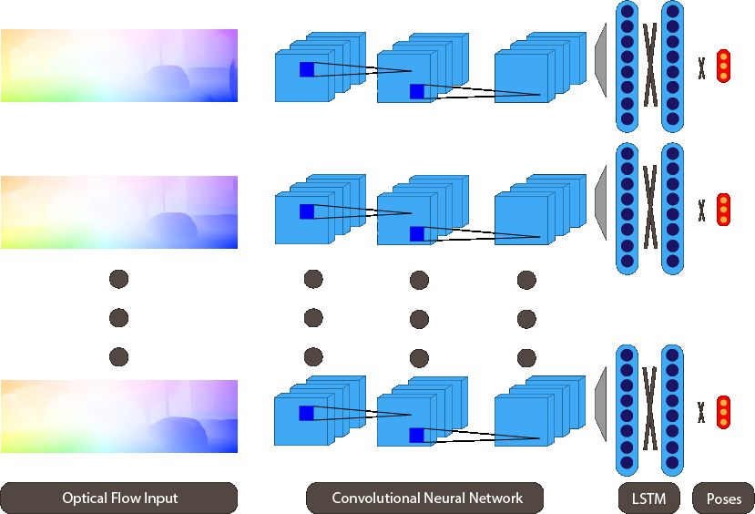
Sensors 2021, 21, 1313                                                                                        4 of 13

                         network designed for learning relationships between RGB pairs may not be sufficient for
                         the task of pose estimation from optical flow, as it was unable to outperform [29].

                         2.3. Contributions
                               Costante et al. [29] argued that CNNs were translation-invariant, and proposed split-
                         ting the optical flow into quadrants to retain motion information. However, their approach
                         was computationally expensive. Thus, our proposed solution is more similar to [26], of
                         conventional regression. However, the approach by Muller and Savakis [26] of adopting
                         the same FlownetS architecture for the task of visual odometry, while promising, could not
                         outperform Costante et al.
                               Deep learning networks, such as Mobilenet [16] and Resnet [17], could outperform
                         traditional approaches for image classification, but not for optical flow estimation. Thus,
                         Flownets [28] came into inception as networks more suitable for the task of optical flow
                         estimation. Now, rather than using Flownets for the task of pose estimation as well, we
                         propose an architecture optimized for estimating relative poses from optical flow.
                               Since the inception of Flownets, there has been an increased interest in augmentation
                         with optical flow in deep learning. It has shown promising results with its introduc-
                         tion in applications such as frame interpolation for slow-motion videos [33] and super-
                         resolution [34]. However, optical flow inputs have underperformed in the field of visual
                         odometry. Our work shows the benefits of optical flow for monocular visual odometry.
                               Wang et al. [24] argued CNNs were insufficient by themselves to model the visual
                         odometry pipeline from raw RGB images, and proposed augmenting CNNs with LSTMs,
                         which can implicitly learn to model the temporal relationship between subsequent frames.
                         To exploit this advantage, we also augment our optical flow-based network with LSTMs to
                         reduce the drift errors in a sequence.

                         3. Visual Odometery Using Optical Flow
                              In our approach, we combine optical flow-based ego-motion estimation with sequence-
                         based modelling. We take in optical flow as input and use CNNs to learn a dense feature
                         description, which is then passed onto bi-LSTMs. Our network models spatio-temporal
                         relationships across a sequence to frame the entire visual odometry pipeline (Figure 1).
                         We show our proposed architecture in Figure 2. However, calculating optical flow [35]
                         has always been a computationally expensive task. Fischer et al. [28] proposed two novel
                         architectures, FlownetS and FlownetC, for estimating the optical flow given two RGB
                         images. While the FlownetS architecture used a single network for feature extraction and
                         matching, FlownetC used a siamese network for feature extraction and a novel correlation
                         layer for feature matching in higher dimensions. The networks were able to deliver
                         competitive results with real-time frame rates. Flownet was followed by Flownet2 [36],
                         which proposed stacking the different architectures together and significantly improved
                         upon optical flow estimates. Since then, there has been an increased interest in leveraging
                         deep learning for predicting optical flow.
                              For our proposed method, we use LiteFlowNet [37] to predict our optical flow input.
                         LiteFlowNet was designed on the principles of pyramid feature scaling, feature warping,
                         and cost volume. Rather than scaling images, feature pyramids are generated at different
                         scales to make the network more robust to noise and changes in illumination. It then uses
                         feature warping to generate a cost volume representation, and introduces a regularization
                         layer to refine the optical flow estimate. LiteFlowNet is 30 times smaller than Flownet2,
                         and outperformed PWC-Net [38] and Flownet2 on the KITTI flow 2012 benchmark [39].
                         We show a visualization of the generated optical flow in Figure 3.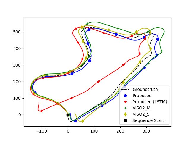
Sensors 2021, 21, 1313                                                                                        5 of 13

                         Figure 2. Proposed architecture.

                                                      (a) Frame at time t.

                                                    (b) Frame at time t + 1.

                                                   (c) Resulting optical flow.

                         Figure 3. Example frames from the KITTI dataset [40] and resulting optical flow using Lite-
                         FlowNet [37].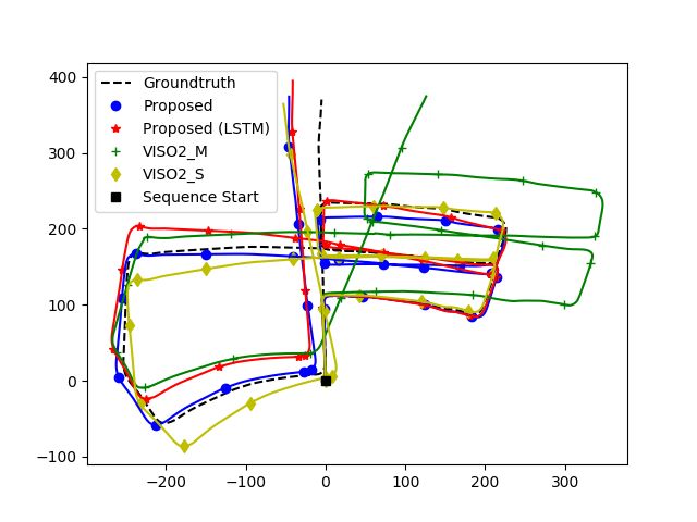
Sensors 2021, 21, 1313                                                                                             6 of 13

                         3.1. Optical Flow
                              The rise in popularity of deep learning for image classification came due to the
                         availability of large-scale datasets. Ideally, we would want our dataset to represent the
                         real world. However, there is a lack of comprehensive data for geometric tasks, such as
                         visual odometry, which require recording and manually calibrating data from different
                         sensors. To overcome this limitation, we chose to work with optical flow rather than RGB
                         images, as optical flow is an encoded representation of flow of motion. It is scene-invariant
                         and maps the pixel correspondences between subsequent frames. We believe an optical
                         flow-based method would generalize better compared to RGB images.

                         3.2. CNN Architecture
                              Extracting features from optical flow is suitable for a CNN, as it requires extracting
                         patterns from encoded flow vectors. However, existing off-the-shelf feature extractors,
                         such as Mobilenet and Resnet, were trained on Imagenet, which is of a different domain.
                         Thus, we propose our own network for extracting features from optical flow. Rather than
                         use the FlownetS architecture which was designed for RGB images, we did a parameter
                         search for a network suitable for optical flow inputs, through hyper-parameter tuning [41].
                         The network consists of seven convolution layers with max pooling applied after every
                         layer, excluding the last one. We apply a rectified linear unit as our activation function. The
                         CNN architecture is described in Table 1. We use a small architecture to avoid the problem
                         of over-fitting, as we are working on a relatively small dataset.

                         Table 1. Structure of CNN.

                                  Layer                Kernel Size               Strides                Channels
                                Conv2D                      3                       1                      16
                                MaxPool                                             2
                                Conv2D                      3                       1                      32
                                MaxPool                                             2
                                Conv2D                      3                       1                      64
                                MaxPool                                             2
                                Conv2D                      3                       1                      128
                                MaxPool                                             2
                                Conv2D                      3                       1                      128
                                MaxPool                                             2
                                Conv2D                      3                       1                      256
                                MaxPool                                             2
                                 Conv2D                     3                       1                      256

                              We pass 2D optical flow vectors as input, where every vector acts as a relative pose for
                         that point in space. At this stage, our network has to implicitly estimate the relative pose for
                         all points and accumulate the results to come up with a final estimate for camera motion.

                         3.3. Sequence-Based Modelling
                              Sequence-based modelling for visual odometry was first proposed by [24]. RNNs
                         have shown remarkable performance on Natural Language Processing (NLP) tasks [42],
                         and have been used extensively for sequence-based learning [43]. RNNs have the ability to
                         learn relationships over time as they can access feature outputs of the previous cell.
                              Given feature xt at time t, RNN is updated at time t by:

                                                         ht = µ(Wxh xt + Whh ht−1 + bh )
                                                                                                                      (1)
                                                                        yt = Why ht + by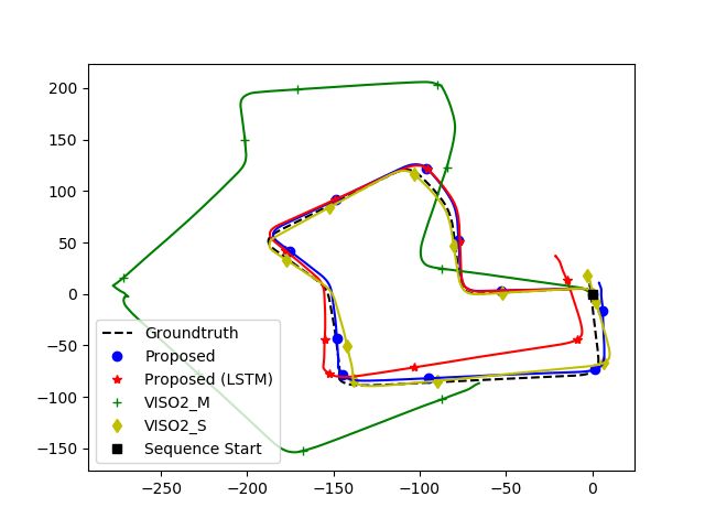
Sensors 2021, 21, 1313                                                                                                7 of 13

                         where ht is the state variable of the hidden layer at time t, yt an output variable. Whh and
                         Wxh are the weight matrix of the hidden layers and input features, respectively, and bh and
                         by are the bias vectors of the hidden layers and input features, respectively. µ is a non-linear
                         activation function, generally consisting of tanh and hard sigmoid.
                              However, RNNs suffer from vanishing gradients if the gradients pass through many
                         timesteps. Thus, to account for the vanishing gradients, LSTMs were introduced with a
                         three-gate system, namely, an input gate, output gate, and a forget gate. The gates deter-
                         mine how to update the current state. LSTMs avoid the problem of vanishing gradients,
                         and can capture relationships over long periods. For our paper, we follow the approach
                         proposed by [25] and use a bi-directional LSTM which consists of two LSTMs.
                              The equations for the input gate, forget gate, output gate, and input cell state are
                         as follows:

                                                            f t = σg (W f xt + U f ht−1 + b f )
                                                              it = σg (Wi xt + Ui ht−1 + bi )
                                                                                                                         (2)
                                                            ot = σg (Wo xt + Uo ht−1 + bo )
                                                         e = tanh(WC xt + Uc ht−1 + bc )
                                                         C
                         where W f , Wi , Wo , and Wc are the weight matrices for the forget gate, input gate, output
                         gate, and input cell state, while U f , Ui , Uo and Uc are the weight matrices connecting the
                         previous cell output state to the three gates and the input cell state. b f , bi , bo and bc are the
                         bias vectors for the forget gate, input gate, output gate, and input cell state. σg is the gate
                         activation function, a hard sigmoid function, and tanh is the hyperbolic tangent function.
                         The cell output state Ct and the hidden state ht are as follows:

                                                                 Ct = f t ∗ Ct−1 + it ∗ C
                                                                                        et
                                                                                                                         (3)
                                                                        ht = ot ∗ tanh(Ct ).
                              Bi-directional LSTMs consists of two LSTMs. Thus, the output is represented as:
                                                                               −
                                                                               → ←    −
                                                                      y t = σ ( h t , h t ),                             (4)
                         where σ is the function used to combine the two output sequences and yt is the output
                         variable at time t.
                                                                                        −
                                                                                        →
                              Bi-directional LSTMs learns from both forward-sequence h from time t1 ...tn , as well
                                                  ←
                                                  −
                         as backward-sequence h from time tn ...t1 .
                              The last layer of our CNN block passes a dense feature representation to the bi-LSTMs
                         to model the temporal relationships between feature representations in higher dimensions.
                              We use a pair of bi-LSTMs as proposed by [24] with 128 units, thus a total of 256 units,
                         and a timestep of five frames. The bi-LSTMs are then connected to a fully connected layer
                         which estimates the 6-DOF pose.

                         3.4. Loss Function
                              We use the Mean Squared Error (MSE) loss to minimize the euclidean distance between
                         the ground-truth pose and prediction:

                                                             N    K
                                                        1
                                                            ∑ ∑ || p̂k
                                                                           (i )      (i )         (i )   (i )
                                               argmin                             − pk ||22 − w||q̂k − qk ||22           (5)
                                                   θ    N   i =1 k =1

                         where p and q denote translation and rotation parameters and N and K the number of
                         samples and dimensions, respectively.
Sensors 2021, 21, 1313                                                                                        8 of 13

                         4. Results
                            In this section, we go over our implementation and training details and evaluate our
                         model on the KITTI dataset [40].

                         4.1. Experimental Setup
                              The network was trained using Tensorflow 2.0 with an Intel i7-6850K, Nvidia Geforce
                         Titan X Maxwell and 32 GBs of RAM.

                         4.2. Dataset
                               The KITTI dataset [40] consists of 22 sequences. Only sequences 00–10 have their
                         ground truth provided. The rest are saved for testing and only supplied with raw sensor
                         data. The dataset includes stereo images captured at 10 fps, as well as IMU and LIDAR.
                         For our purposes, we only work with the left-most stereo camera. The dataset consists of a
                         car driving in dense residential urban environments and sparse highways. To train our
                         model, we divide the dataset into training and testing data. We use sequences 00, 02, 04,
                         06, 08, and 10 for training our model and sequences 03, 05, 07, and 09 for validation. We
                         avoid working with sequence 01 since the car is driving at high speeds, resulting in large
                         displacements between frames.
                               The ground-truth is comprised of 4 × 4 transformation matrices. We calculate the
                         relative poses for each RGB pair and convert them to an euler representation comprised of
                         three translation and rotation parameters each.

                         4.3. Implementation
                               We use the Adam optimizer with a learning rate of 0.001. Learning rate decay is
                         employed to achieve faster convergence, and the network is trained for 100 epochs. We
                         first train the network to infer relative poses from optical flow, and then augment it with
                         bi-directional LSTMs.

                         4.4. Results
                              We evaluate our model on sequences 03, 05, 07, and 09 to realize the generalization of
                         our network. The evaluation is based on the KITTI odometry benchmark [39]. Translation
                         and rotation errors are calculated for sub-sequences of lengths ranging from 100 to 800 m
                         every 100 m. Then, the averaged root-mean-squared error is considered. We compare our
                         results vs. VISO2 [13] and MagicVO [25]. VISO2 is an open-source, feature-based solution
                         for visual odometry. It minimizes re-projection errors between sparse feature matches
                         and supports monocular and stereo-based configurations. We show comparisons against
                         both configurations. MagicVO is a deep learning approach that augments FlownetS with
                         bi-directional LSTMs. We chose to compare against MagicVO, as their results outperform
                         other approaches in the literature, and thus they act as a good baseline. Since their
                         implementation is not public, we compare against results published in their paper. We
                         report our results in Table 2. We also draw a quantitative and qualitative comparison
                         against VISO2. We show quantitative comparisons in Figure 4, and qualitative ones in
                         Figure 5.
Sensors 2021, 21, 1313 9 of 13
Table 2. Comparison of proposed method vs. monocular and stereo-based VISO2 and MagicVO. • t: average translation
drift (%) on length of 100–800 m. • r: average rotation drift (◦ /100 m) on length of 100–800 m.
Seq. Proposed Proposed (LSTM) VISO2_M VISO2_S MagicVO
t (%) r (◦ ) t (%) r (◦ ) t (%) r (◦ ) t (%) r (◦ ) t (%) r (◦ )
03 4.85 2.54 9.82 3.64 10.57 1.73 2.94 1.09 4.95 2.44
05 2.89 1.22 3.03 1.23 19.02 4.21 2.40 1.15 1.63 2.25
07 2.56 2.15 6.43 3.39 34.16 9.98 2.67 1.61 2.61 1.08
09 2.54 0.90 5.05 1.90 5.76 1.05 2.86 1.14 5.43 2.27
Avg. 3.21 1.70 6.08 2.54 17.38 4.24 2.72 1.25 3.66 2.01
(a) Translation Error vs. Path Length (b) Translation Error vs. Speed
(c) Rotation Error vs. Path Length (d) Rotation Error vs. Speed
Figure 4. Comparison of the proposed method based on the KITTI evaluation kit.Sensors 2021, 21, 1313 10 of 13
(a) Sequence 03 (b) Sequence 05
(c) Sequence 07 (d) Sequence 09
Figure 5. Comparison of our proposed method with VISO2.
4.5. Analysis
The averaged quantitative results are given in Table 2. We outperformed our monoc-
ular baselines (VISO2_M, MagicVO) on unknown environments and came close to the
stereo-based approach (VISO_S). The stereo-based configuration uses multiple perspectives
for better scene understanding and reduces the error caused by drift, while our approach
uses deep learning to generate robust spatio-temporal feature descriptions, significantly
outperforming traditional monocular methods.
The dataset consists of dynamic scenes with multiple moving objects, and was cap-
tured at 10 fps with the car moving at high speeds. This results in large displacements
between frames. It can prove challenging for traditional feature-based approaches to
perform feature-matching between distant frames. A neural network might prove to be
invariant to such faults, as the network takes many features into consideration.
Interestingly, LSTMs reduced our accuracy in a counter-intuitive manner. While the
LSTMs managed to model the relationships between RGB image pairs, they fail to do so
when working with optical flow images. This could be due to the prevalence of temporal
feature representations, since RGB image pairs use the same image twice when iterating
through a sequence, which is missing when working with optical flow since optical flow
is scene-invariant. Subsequent optical flows can differ, whereas the RGB frame at time tSensors 2021, 21, 1313 11 of 13
will be shared with both the frames at time t − 1 and t + 1. Figure 4b,d indicates that using
LSTMs helped at high speeds when there are large displacements between frames, and it is
able to use sequential information to output an improved estimate. There are also limited
samples in the dataset with the car driving at speeds greater than 50 or slower than 20. We
believe more experimentation is required in assessing the role of LSTMs when working
with optical flow feature representations.
Figure 5 also indicates the errors are not evenly distributed. While straight roads
show little divergence, errors around turns and corners are high, which skews the global
trajectory when a turn is encountered. Figure 4b,d shows errors increase significantly when
the car is moving at a slow speed. Most of the samples consist of the car driving in a straight
manner with uniform speed. The car occasionally slows down to turn or come to a stop.
The lack of balanced data is a big drawback for deep learning against a stereo baseline.
With errors concentrated around turns, some frames contribute more to the relative
errors which get accumulated over a trajectory. A loss function that can explicitly enforce
the relationship between subsequent frames and weigh the contribution of each frame
would be ideal. The averaged root-mean-square error is not sufficient where data are
not weighted uniformly. Conventional methods perform feature extraction and evaluate
whether a frame is viable for pose estimation and can contribute to the global trajectory.
However, a neural network, when given an input, will always provide an output. Neural
networks assume all inputs have an equal contribution. A biased network that can weight
the input can get better results.
5. Conclusions
In this paper, we presented a deep learning-based solution for visual odometry (VO).
We validated that CNNs are capable of predicting camera motion with only optical flow as
input. Our proposed solution outperformed MagicVO, which used features extracted from
RGB images and modelled the VO pipeline using bi-directional LSTMs.
While our initial experiments surpassed VISO2_M and MagicVO (monocular base-
lines), the stereo-based approach still scored better. Additionally, augmenting our approach
with LSTMs showed interesting behaviour that we would like to pursue in further studies.
However, we believe that a bigger dataset would help in achieving better results.
For future work, we will test and validate our network on more datasets. We will also
explore the architecture search space for a network with an induction bias more tuned for
visual odometry.
Author Contributions: Conceptualization and Literature Review, T.P. and D.P.; Methodology and
Experimentation, T.P.; Review, D.P. and J.B.; Supervision D.P., J.B., D.M. All authors have read and
agreed to the published version of the manuscript.
Funding: This research received no external funding.
Institutional Review Board Statement: Not applicable.
Informed Consent Statement: Not applicable.
Data Availability Statement: The KITTI Dataset [40] used for this study can be accessed at http:
//www.cvlibs.net/datasets/kitti/ (accessed on 27 January 2021).
Conflicts of Interest: The authors declare no conflict of interest.
References
1. Scaramuzza, D.; Fraundorfer, F. Visual Odometry [Tutorial]. IEEE Robot. Autom. Mag. 2011, 18, 80–92. [CrossRef]
2. Yang, C.; Mark, M.; Larry, M. Visual odometry on the Mars Exploration Rovers. In Proceedings of the 2005 IEEE International
Conference on Systems, Man and Cybernetics, Waikoloa, HI, USA, 12 October 2005; Volume 1, pp. 903–910. [CrossRef]
3. Corke, P.; Strelow, D.; Singh, S. Omnidirectional visual odometry for a planetary rover. In Proceedings of the 2004 IEEE/RSJ
International Conference on Intelligent Robots and Systems (IROS) (IEEE Cat. No.04CH37566), Sendai, Japan, 28 September–2
October 2004; Volume 4, pp. 4007–4012. [CrossRef]Sensors 2021, 21, 1313 12 of 13
4. Howard, A. Real-time stereo visual odometry for autonomous ground vehicles. In Proceedings of the 2008 IEEE/RSJ International
Conference on Intelligent Robots and Systems, Nice, France, 22–26 September 2008; pp. 3946–3952. [CrossRef]
5. Wang, R.; Schworer, M.; Cremers, D. Stereo DSO: Large-Scale Direct Sparse Visual Odometry With Stereo Cameras. arXiv 2017,
arXiv:1708.07878.
6. Huang, A.S.; Bachrach, A.; Henry, P.; Krainin, M.; Fox, D.; Roy, N. Visual odometry and mapping for autonomous flight using an
RGB-D camera. In Robotics Research; Christensen, H., Khatib, O., Eds.; Springer Tracts in Advanced Robotics; Springer: Cham,
Switzerland, 2011; Volume 100.
7. Kerl, C.; Sturm, J.; Cremers, D. Robust odometry estimation for RGB-D cameras. In Proceedings of the 2013 IEEE International
Conference on Robotics and Automation, Karlsruhe, Germany, 6–10 May 2013; pp. 3748–3754. [CrossRef]
8. Leutenegger, S.; Lynen, S.; Bosse, M.; Siegwart, R.; Furgale, P. Keyframe-based visual–inertial odometry using nonlinear
optimization. Int. J. Robot. Res. 2015, 34, 314–334. [CrossRef]
9. Bloesch, M.; Omari, S.; Hutter, M.; Siegwart, R. Robust visual inertial odometry using a direct EKF-based approach. In
Proceedings of the 2015 IEEE/RSJ International Conference on Intelligent Robots and Systems (IROS), Hamburg, Germany, 28
September–2 October 2015; pp. 298–304. [CrossRef]
10. Yang, N.; Wang, R.; Gao, X.; Cremers, D. Challenges in Monocular Visual Odometry: Photometric Calibration, Motion Bias, and
Rolling Shutter Effect. IEEE Robot. Autom. Lett. 2018, 3, 2878–2885. [CrossRef]
11. Nister, D.; Naroditsky, O.; Bergen, J. Visual odometry. In Proceedings of the 2004 IEEE Computer Society Conference on
Computer Vision and Pattern Recognition, 2004. CVPR 2004, Washington, DC, USA, 27 June–2 July 2004; Volume 1, p. I.
[CrossRef]
12. Mur-Artal, R.; Montiel, J.M.M.; Tardós, J.D. ORB-SLAM: A Versatile and Accurate Monocular SLAM System. arXiv 2015,
arXiv:1502.00956.
13. Geiger, A.; Ziegler, J.; Stiller, C. StereoScan: Dense 3d reconstruction in real-time. In Proceedings of the 2011 IEEE Intelligent
Vehicles Symposium (IV), Baden, Germany, 5–9 June 2011; pp. 963–968. [CrossRef]
14. Harris, C.; Stephens, M. A combined corner and edge detector. In Proceedings of the Alvey Vision Conference, Manchester, UK,
31 August–2 September 1988; pp. 147–151.
15. Engel, J.; Koltun, V.; Cremers, D. Direct Sparse Odometry. arXiv 2016, arXiv:1607.02565.
16. Howard, A.G.; Zhu, M.; Chen, B.; Kalenichenko, D.; Wang, W.; Weyand, T.; Andreetto, M.; Adam, H. MobileNets: Efficient
Convolutional Neural Networks for Mobile Vision Applications. arXiv 2017, arXiv:1704.04861v1.
17. He, K.; Zhang, X.; Ren, S.; Sun, J. Deep Residual Learning for Image Recognition. arXiv 2015, arXiv:1512.03385v1.
18. Szegedy, C.; Liu, W.; Jia, Y.; Sermanet, P.; Reed, S.E.; Anguelov, D.; Erhan, D.; Vanhoucke, V.; Rabinovich, A. Going Deeper with
Convolutions. arXiv 2014, arXiv:1409.4842.
19. Sabour, S.; Frosst, N.; Hinton, G.E. Dynamic Routing Between Capsules. arXiv 2017, arXiv:1710.09829.
20. Pan, X.; Shi, J.; Luo, P.; Wang, X.; Tang, X. Spatial As Deep: Spatial CNN for Traffic Scene Understanding. arXiv 2017,
arXiv:1712.06080.
21. Fraundorfer, F.; Scaramuzza, D. Visual Odometry: Part II: Matching, Robustness, Optimization, and Applications. IEEE Robot.
Autom. Mag. 2012, 19, 78–90. [CrossRef]
22. Forster, C.; Pizzoli, M.; Scaramuzza, D. SVO: Fast semi-direct monocular visual odometry. In Proceedings of the 2014 IEEE
International Conference on Robotics and Automation (ICRA), Hong Kong, China, 31 May–7 June 2014; pp. 15–22. [CrossRef]
23. Engel, J.; Cremers, D. LSD-SLAM: Large-scale direct monocular SLAM. In Computer Vision—ECCV 2014; Lecture Notes in
Computer Science; Fleet, D., Pajdla, T., Schiele, B., Tuytelaars, T., Eds.; Springer: Cham, Switzerland, 2014; Volume 8690.
24. Wang, S.; Clark, R.; Wen, H.; Trigoni, N. DeepVO: Towards End-to-End Visual Odometry with Deep Recurrent Convolutional
Neural Networks. arXiv 2017, arXiv:1709.08429.
25. Jiao, J.; Jiao, J.; Mo, Y.; Liu, W.; Deng, Z. MagicVO: An End-to-End Hybrid CNN and Bi-LSTM Method for Monocular Visual
Odometry. IEEE Access 2019, 7, 94118–94127. [CrossRef]
26. Muller, P.; Savakis, A. Flowdometry: An Optical Flow and Deep Learning Based Approach to Visual Odometry. In Proceedings
of the 2017 IEEE Winter Conference on Applications of Computer Vision (WACV), Santa Rosa, CA, USA, 24–31 March 2017;
pp. 624–631. [CrossRef]
27. Parisotto, E.; Chaplot, D.S.; Zhang, J.; Salakhutdinov, R. Global Pose Estimation with an Attention-based Recurrent Network.
arXiv 2018, arXiv:1802.06857.
28. Fischer, P.; Dosovitskiy, A.; Ilg, E.; Häusser, P.; Hazirbas, C.; Golkov, V.; van der Smagt, P.; Cremers, D.; Brox, T. FlowNet: Learning
Optical Flow with Convolutional Networks. arXiv 2015, arXiv:1504.06852.
29. Costante, G.; Mancini, M.; Valigi, P.; Ciarfuglia, T.A. Exploring Representation Learning With CNNs for Frame-to-Frame
Ego-Motion Estimation. IEEE Robot. Autom. Lett. 2016, 1, 18–25. [CrossRef]
30. Costante, G.; Ciarfuglia, T.A. LS-VO: Learning Dense Optical Subspace for Robust Visual Odometry Estimation. arXiv 2017,
arXiv:1709.06019.
31. Mur-Artal, R.; Tardós, J.D. ORB-SLAM2: An Open-Source SLAM System for Monocular, Stereo and RGB-D Cameras. arXiv 2016,
arXiv:1610.06475.
32. Sener, O.; Koltun, V. Multi-Task Learning as Multi-Objective Optimization. arXiv 2018, arXiv:1810.04650v2.Sensors 2021, 21, 1313 13 of 13
33. Jiang, H.; Sun, D.; Jampani, V.; Yang, M.; Learned-Miller, E.G.; Kautz, J. Super SloMo: High Quality Estimation of Multiple
Intermediate Frames for Video Interpolation. arXiv 2018, arXiv:1712.00080.
34. DLSS 2.0—Image Reconstruction for Real-Time Rendering with Deep Learning. Available online: https://www.nvidia.com/en-
us/on-demand/session/gtcsj20-s22698/ (accessed on 27 January 2021).
35. Barron, J.L.; Fleet, D.J.; Beauchemin, S.S. Performance of Optical Flow Techniques. Int. J. Comput. Vision 1994, 12, 43–77.
[CrossRef]
36. Ilg, E.; Mayer, N.; Saikia, T.; Keuper, M.; Dosovitskiy, A.; Brox, T. FlowNet 2.0: Evolution of Optical Flow Estimation with Deep
Networks. arXiv 2016, arXiv:1612.01925.
37. Hui, T.; Tang, X.; Loy, C.C. LiteFlowNet: A Lightweight Convolutional Neural Network for Optical Flow Estimation. arXiv 2018,
arXiv:1805.07036.
38. Sun, D.; Yang, X.; Liu, M.; Kautz, J. PWC-Net: CNNs for Optical Flow Using Pyramid, Warping, and Cost Volume. arXiv 2017,
arXiv:1709.02371.
39. Geiger, A.; Lenz, P.; Urtasun, R. Are we ready for Autonomous Driving? The KITTI Vision Benchmark Suite. In Proceedings of
the Conference on Computer Vision and Pattern Recognition (CVPR), Providence, RI, USA, 16–21 June 2012.
40. Geiger, A.; Lenz, P.; Stiller, C.; Urtasun, R. Vision meets Robotics: The KITTI Dataset. Int. J. Robot. Res. (IJRR) 2013. [CrossRef]
41. O’Malley, T.; Bursztein, E.; Long, J.; Chollet, F.; Jin, H.; Invernizzi, L. Keras Tuner. Available online: https://github.com/keras-
team/keras-tuner (accessed on 5 August 2020).
42. Graves, A.; Mohamed, A.; Hinton, G.E. Speech Recognition with Deep Recurrent Neural Networks. arXiv 2013, arXiv:1303.5778.
43. Lipton, Z.C. A Critical Review of Recurrent Neural Networks for Sequence Learning. arXiv 2015, arXiv:1506.00019.You can also read