Generalizing Deep Models for Overhead Image Segmentation Through Getis-Ord Gi* Pooling - DROPS
←
→
Page content transcription
If your browser does not render page correctly, please read the page content below
Generalizing Deep Models for Overhead Image
Segmentation Through Getis-Ord Gi* Pooling
Xueqing Deng
EECS, University of California, Merced, CA, USA
xdeng7@ucmerced.edu
Yuxin Tian
EECS, University of California, Merced, CA, USA
ytian8@ucmerced.edu
Shawn Newsam
EECS, University of California, Merced, CA, USA
snewsam@ucmerced.edu

      Abstract
That most deep learning models are purely data driven is both a strength and a weakness. Given
sufficient training data, the optimal model for a particular problem can be learned. However, this is
usually not the case and so instead the model is either learned from scratch from a limited amount of
training data or pre-trained on a different problem and then fine-tuned. Both of these situations are
potentially suboptimal and limit the generalizability of the model. Inspired by this, we investigate
methods to inform or guide deep learning models for geospatial image analysis to increase their
performance when a limited amount of training data is available or when they are applied to scenarios
other than which they were trained on. In particular, we exploit the fact that there are certain
fundamental rules as to how things are distributed on the surface of the Earth and these rules do not
vary substantially between locations. Based on this, we develop a novel feature pooling method for
convolutional neural networks using Getis-Ord G∗i analysis from geostatistics. Experimental results
show our proposed pooling function has significantly better generalization performance compared to
a standard data-driven approach when applied to overhead image segmentation.

2012 ACM Subject Classification Computing methodologies → Neural networks

Keywords and phrases Remote sensing, convolutional neural networks, pooling function, semantic
segmentation, generalization

Digital Object Identifier 10.4230/LIPIcs.GIScience.2021.I.3

Funding This work was funded in part by a National Science Foundation grant, #IIS-1747535.

Acknowledgements We gratefully acknowledge the support of NVIDIA Corporation through the
donation of the GPU card used in this work. And we thank Yi Zhu for providing helpful discussion.

 1      Introduction
Research in remote sensing has been steadily increasing since it is an important source for
Earth observation. Overhead imagery can easily be acquired using low-cost drones and no
longer requires access to expensive high-resolution satellite or airborne platforms. Since
the data provides convenient and large-scale coverage, people are using it for a number of
societally important problems such as traffic monitoring [20], land cover segmentation [16],
building extraction [10, 37], geolocalization [31], image retrieval [27], etc.
   Recently, the analysis of overhead imagery has benefited greatly from deep learning
thanks to the significant advancements made by the computer vision community on regular
(non-overhead) images. However, there still often remains challenges when adapting these
deep learning techniques to overhead image analysis, such as the limited availability of labeled
overhead imagery, the difficulty of the models to generalize between locations, etc.
            © Xueqing Deng, Yuxin Tian, and Shawn Newsam;
            licensed under Creative Commons License CC-BY
11th International Conference on Geographic Information Science (GIScience 2021) – Part I.
Editors: Krzysztof Janowicz and Judith A. Verstegen; Article No. 3; pp. 3:1–3:14
                   Leibniz International Proceedings in Informatics
                   Schloss Dagstuhl – Leibniz-Zentrum für Informatik, Dagstuhl Publishing, Germany
3:2   Generalizing Deep Models for Through G-Pooling

          Annotating overhead imagery is labor intensive so existing datasets are often not large
      enough to train effective convolutional neural networks (CNNs) from scratch. A common
      practice therefore is to fine-tune an ImageNet pre-trained model on a small amount of
      annotated overhead imagery. However, the generalization capability of fine-tuned models is
      limited as models trained on one location may not work well on others. This is known as
      the cross-location generalization problem and is not necessarily limited to overhead image
      analysis as it can also be a challenge for ground-level imagery such as cross-city road scene
      segmentation [9]. Deep models are often overfit due to their large capacity yet generalization
      is particularly important for overhead images since they can look quite different due to
      variations in the seasons, position of the sun, location variation, etc. For regular image
      analysis, two widely adopted approaches to overcome these so-called domain gaps include
      domain adaptation [11, 12, 33–35] and data fusion. Both approaches have been adapted by
      the remote sensing community [2] to improve performance and robustness.
          In this paper, we take a different, novel approach to address the domain gap problem.
      We exploit the fact that things are not laid out at random on the surface of the Earth and
      that this structure does not vary substantially between locations. In particular, we pose the
      question of how prior knowledge of this structure or, more interestingly, how the fundamental
      rules of geography, might be incorporated into general CNN frameworks. Inspired by work
      on physics-guided neural networks [14], we develop a framework in which spatial hotspot
      analysis informs the feature map pooling. We term this geo-constrained pooling strategy
      Getis-Ord G∗i pooling and show that it significantly improves the semantic segmentation of
      overhead imagery particularly in cross-location scenarios. To our knowledge, ours is the
      first work to incorporate geo-spatial knowledge directly into the fundamental mechanisms
      of CNNs.
           Our contributions are summarized as follows:
      1. We propose Getis-Ord G∗i pooling, a novel pooling method based on spatial Getis-Ord G∗i
         analysis of CNN feature maps. Getis-Ord G∗i pooling is shown to significantly improve
         model generalization for overhead image segmentation.
      2. We establish more generally that using geospatial knowledge in the design of CNNs can
         improve the generalizability of the models.

       2      Related Work

      Semantic segmentation. Fully connected neural networks (FCN) were recently proposed
      to improve the semantic segmentation of non-overhead imagery [19]. Various techniques
      have been proposed to boost their performance, such as atrous convolution [5–7, 40], skip
      connections [25] and preserving max pooling index for unpooling [3]. And, recently, video has
      been used to scale up training sets by synthesizing new training samples [42]. Remote sensing
      research has been driven largely by adapting advances in regular image analysis to overhead
      imagery. In particular, deep learning approaches to overhead image analysis have become
      a standard practice for a variety of tasks, such as land use/land cover classification [16],
      building extraction [37], road segmentation [22], car detection [8], etc. More literature can
      be found in a recent survey [41]. And various segmentation networks have been proposed,
      such relation-augmentation networks [23] and ScasNet [18]. However, these methods only
      adapt deep learning techniques and networks from regular to overhead images–they do not
      incorporate geographic structure or knowledge.
X. Deng, Y. Tian, and S. Newsam 3:3
Knowledge guided neural networks. Analyzing overhead imagery is not just a computer
vision problem since the principles of the physical world such as geo-spatial relationships can
help. For example, knowing the road map of a city can improve tasks like building extraction
or land cover segmentation. While there are no works directly related to ours, there have been
some initial attempts to incorporate geographic knowledge into deep learning [4, 39]. Chen et
al. [4] develop a knowledge-guided golf course detection approach using a CNN fine-tuned
on temporally augmented data. They also apply area-based rules during a post-processing
step. Zhang et al. [39] propose searching for adjacent parallel line segments as prior spatial
information for the fast detection of runways. However, these methods simply fuse prior
knowledge from other sources. Our proposed method is novel in that we incorporate geo-
spatial rules into the CNN mechanics. We show later how this helps regularize the model
and leads to better generalization.
Pooling functions. A number of works have investigated different pooling methods for
image classification and segmentation tasks. The Lp norm has been proposed to extend max
pooling where intermediate pooling functions are manually selected between max and average
pooling to better fit the distribution of the input data. [17] generalizes pooling methods by
using a learned linear combination of max and average pooling. Detail-Preserving Pooling
(DPP) [26] learns weighted summations of pixels over different pooling regions. Salient pixels
are considered more important and thus given higher weighting. Strided convolution has been
used to replace all max pooling layers and activation functions in a small classification model
that is trained from scratch and has shown to improve performance [30]. Strided convolution
is common in segmentation tasks. For example, the DeepLab series of networks [6, 7] use
strided convolutional layers for feature down-sampling rather than max pooling. To enhance
detail preservation in segmentation, a recent polynomial pooling approach is proposed in [36].
However, all these pooling methods are based on non-spatial statistics. We instead incorporate
geo-spatial rules/knowledge to perform the pooling and downsampling.
3 Methods
In this section, we investigate how geo-spatial knowledge can be incorporated into standard
deep CNNs. We discuss some general rules from geography to describe geo-spatial patterns
on the Earth. Then we propose using Getis-Ord G∗i analysis, a common technique for
geo-spatial clustering, to encapsulate these rules. This then informs our pooling function
which is general and can be used in most network architectures.
3.1 Getis-Ord G∗i pooling (G-pooling)
We take inspiration from the well-known first law of geography: everything is related to
everything else, but near things are more related than distant things [32]. While this rule is
very general and abstract, it motivates a number of quantitative frameworks that have been
shown to improve geospatial data analysis. For example, it motivates spatial autocorrelation
which is the basis for spatial prediction models like kriging. It also motivates the notion of
spatial clustering wherein similar things that are spatially nearby are more significant than
isolated things. Our proposed framework exploits this to introduce a novel feature pooling
method which we term Getis-Ord G∗i pooling.
Pooling is used to spatially downsample the feature maps in deep CNNs. In contrast
to standard image downsampling methods which seek to preserve the spatial envelope of
pixel values, pooling selects feature values that are more significant in some sense. The most
GIScience 20213:4 Generalizing Deep Models for Through G-Pooling
Sliding window
Input feature maps: Max pooling:
!-pooling:
Figure 1 Given a feature map as an input, max pooling (top right) and the proposed G-pooling
(bottom right) produce different downsampled output feature maps. G-pooling exploits spatial
clusters of input feature map values. For example, the feature map within the sliding window (dotted
blue line) indicates a spatial cluster. Max pooling takes the max value ignoring the spatial cluster,
while our G-pooling takes the interpolated value at the center location. (White, gray and black
represent three ranges of feature map values, from low to high.)
standard pooling method is max pooling in which the maximum feature value in a window
is propagated. Other pooling methods have been proposed. Average pooling is an obvious
choice and is used in [13, 38] for image classification. Strided convolution [15] has also been
used. However, max pooling remains by far the most common as it has the intuitive appeal
of extracting the maximum activation and thus the most prominent features.
However, we postulate that isolated high feature values might not be the most informative
and instead develop a method to propagate clustered values. Specifically, we use a technique
from geostatistics termed hotspot analysis to identify clusters of large positive values and
then propagate a representative from these clusters. Hotspot analysis uses the Getis-Ord
G∗i [24] statistic to find locations that have either high or low values and are surrounded
by locations also with high or low values. These locations are the so-called hotspots. The
Getis-Ord G∗i statistic is computed by comparing the local sum of a feature and its neighbors
proportionally to the sum of all features in a spatial region. When the local sum is different
from the expected local sum, and when that difference is too large to be the result of random
noise, it will lead to a high positive or low negative G∗i value that is statistically significant.
We focus on locations with high positive G∗i values since we want to propagate activations.
3.2 Definition
We now describe our G-pooling algorithm in detail. Please see Figure 1 for reference. Similar
to other pooling methods, we use a sliding window to downsample the input. Given a feature
map within the window, in order to compute its G∗i , we first need to define the weight matrix
based on the spatial locations.
We denote the feature values within the sliding window as X = x1 , x2 , ..., xn where n
is the number of pixels (locations) within the sliding window. We assume the window is
rectangular and compute the G∗i statistic at the center of the window. Let the feature value
at the center be xi . (If the center does not fall on a pixel location then we compute xiX. Deng, Y. Tian, and S. Newsam 3:5
as the average of the adjacent values.) The G∗i statistic uses weighed averages where the
weights are based on spatial distances. Let px (xj ) and py (xj ) denote the x and y positions
of feature value xj in the image plane. A weight matrix w that measures the Euclidean
distance on the image plane between xi and the other locations within the sliding window is
then computed as
q
wi,j = (px (xi ) − px (xj ))2 + (py (xi ) − py (xj ))2 . (1)
The Getis-Ord G∗i value at location i is now computed as
Pn Pn
∗ j=1 wi,j xj − X̄ j=1 wi,j
Gi = r Pn Pn . (2)
[n 2
wi,j −( wi,j )2 ]
j=1 j=1
S n−1
where X̄ and S are as below,
Pn
j=1 xj
X̄ = , (3)
n
sP
n
j=1 x2j
S= − (X̄)2 . (4)
n
Spatial clusters can be detected based on the G∗i value. The higher the value, the more
significant the cluster is. However, the G∗i value just indicates whether there is a spatial
cluster or not. To achieve our goal of pooling, we need to summarize the local region of
the feature map by extracting a representative value. We use a threshold to do this. If the
computed G∗i is greater than or equal to the threshold, a spatial cluster is detected and the
value xi is used for pooling; otherwise the maximum value in the window is used:
(
xi if G∗i ≥ threshold
G − pooling(x) = (5)
max(x) if G∗i < threshold
G∗i is in range [-2.8,2.8] for our particular range of feature map values. A positive value
indicates a hotspot which is a cluster of positive values, a negative value indicates a coldspot
which is a cluster of negative values, and values near zero indicate scatter. The absolute
value |G∗i | indicates the significance of the cluster. For example, a high positive G∗i value
indicates the location is more likely to be a spatial cluster of high positive values.
The output feature map produced by G-pooling is G-pooling(X) which results after sliding
the window over the entire input feature map. We experiment with three threshold values:
1.0, 1.5, 2.0. A higher threshold value results in fewer spatial clusters and so max pooling
will be applied more often. A lower threshold value results in more spatial clusters and so
max pooling will be applied less often. As the threshold ranges from 1.0 to 1.5 to 2.0, fewer
spatial clusters/hotspots will be detected. We find that a threshold of 2.0 results in few
hostpots being detected and max pooling primarily being used.
3.3 Network Architecture
A pretrained VGG network [29] is used in our experiments. VGG has been widely used as
a backbone in various semantic segmentation networks such as FCN [19], U-net [25], and
SegNet [3]. In VGG, the standard max pooling is a 2×2 window size with a stride of 1. Our
GIScience 20213:6 Generalizing Deep Models for Through G-Pooling
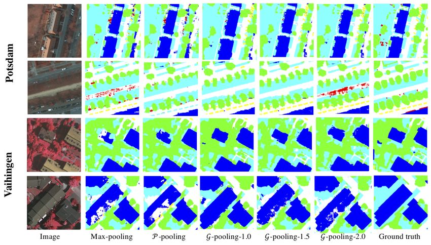
Figure 2 FCN network architecture with G-pooling.
proposed G-pooling uses a 4×4 window size with a stride of 4. Therefore, in standard pooling,
the feature maps are reduced by a factor of 2, while in our G-pooling, they are reduced by a
factor of 4. A larger window is used in our proposed G-pooling since Getis-Ord G∗i analysis
is not as meaningful for small regions. However, we evaluated the scenario in which standard
pooling is also performed with a 4 × 4 sliding window and the performance is only slightly
different from using a standard 2 × 2 window. In general, segmentation networks using
VGG16 as the backbone have 5 max pooling layers, each of which downsamples by a factor of
2. So, when we replace max pooling with our proposed G-pooling, our architecture has two
G-pooling and one max pooling layers in order to produce the same sized final feature map.
Table 1 Training and test data are from the same location. These results are for a FCN using
VGG-16 as the backbone. Stride conv, P-pooling and our approach, G-pooling, are used to replace
the standard max/average pooling. The per class results are reported as IoU. mIoU is the average
across classes. Pixel Acc. is the overall pixel accuracy. Higher is better for all results.
Potsdam
Methods Roads Buildings Low Veg. Trees Cars mIoU Pixel Acc.
Max 70.62 74.28 65.94 61.36 61.40 66.72 79.55
Average 69.34 74.49 63.94 60.06 60.28 65.62 78.08
Stride 67.22 73.97 63.01 60.09 59.39 64.74 77.54
P-pooling 71.97 75.55 66.80 62.03 62.39 67.75 81.02
G-pooling-1.0 (ours) 68.59 77.39 67.48 55.56 62.18 66.24 79.43
G-pooling-1.5 (ours) 70.06 76.12 67.67 62.12 63.91 67.98 81.63
G-pooling-2.0 (ours) 70.99 74.89 65.34 61.57 60.77 66.71 79.46
Vaihingen
Max 70.63 80.42 51.57 70.12 55.32 65.61 81.88
Average 70.54 79.86 50.49 69.18 54.83 64.98 79.98
Strde conv 68.36 77.65 49.21 67.34 53.29 63.17 79.44
P-pooling 71.06 80.52 51.70 70.93 53.65 65.57 82.44
G-pooling-1.0 (ours) 72.15 79.69 53.28 70.89 53.72 65.95 81.78
G-pooling-1.5 (ours) 71.61 78.74 48.18 68.53 55.64 64.54 80.42
G-pooling-2.0 (ours) 71.09 78.88 50.62 68.32 54.01 64.58 80.75X. Deng, Y. Tian, and S. Newsam 3:7
4 Experiments
4.1 Dataset
ISPRS dataset. We evaluate our method on two image datasets from the ISPRS 2D
Semantic Labeling Challenge [1]. These datasets are comprised of very high resolution aerial
images over two cities in Germany: Vaihingen and Potsdam. While Vaihingen is a relatively
small village with many detached buildings and small multi-story buildings, Potsdam is a
typical historic city with large building blocks, narrow streets and dense settlement structure.
The goal is to perform semantic labeling of the images using six common land cover classes:
buildings, impervious surfaces (e.g. roads), low vegetation, trees, cars and clutter/background.
We report test metrics obtained on the held-out test images.
Vaihingen. The Vaihingen dataset has a resolution of 9 cm/pixel with tiles of approximately
2100 × 2100 pixels. There are 33 images, for which 16 have a public ground truth. Even
though the tiles consist of Infrared-Red-Green (IRRG) images and DSM data extracted from
the Lidar point clouds, we use only the IRRG images in our work. We select five images for
validation (IDs: 11, 15, 28, 30 and 34) and the remaining 11 for training, following [21, 28].
Potsdam. The Potsdam dataset has a resolution of 5 cm/pixel with tiles of 6000 × 6000
pixels. There are 38 images, for which 24 have public ground truth. Similar to Vaihingen, we
only use the IRRG images. We select seven images for validation (IDs: 2_11, 2_12, 4_10,
5_11, 6_7, 7_8 and 7_10) and the remaining 17 for training, again following [21, 28].
4.2 Experimental Settings
We first compare our G-pooling to standard max-pooling, average-pooling, strided convolution
and the recently proposed P-pooling [36], all using an FCN semantic segmentation network
with a VGG backbone. We later perform experiments using other semantic segmentation
networks. We compare to max/average pooling as they are commonly used for downsampling
semantic segmentation networks that have VGG as a backbone. Strided convolution has
been used to replace max pooling in recent semantic segmentation frameworks such as the
DeepLab series [5–7] and PSPNet [40]. Detail preserving pooling (DPP) has also been used
to replace standard pooling in works such as DDP [26] and P-pooling [36]. We compare
to the most recent, P-pooling, as it has been shown to outperform other detail preserving
methods.
4.3 Evaluation Metrics
We have two goals in this work, the model’s segmentation accuracy and its generalization
performance. We report model accuracy as the performance on a test/validation set when the
model is trained using training data from the same location (the same dataset). We report
model generalizability as the performance on a test/validation set when the model is trained
using training data from a different location (a different dataset). In general, the domain
gap between the training and test/validation sets is small when they are from the same
location/dataset. However, cross-location/dataset testing can result in large domain shifts.
Model accuracy. The commonly used per class intersection over union (IoU) and mean
IoU (mIoU) as well as the pixel accuracy are adopted for evaluating segmentation accuracy.
IoU is commonly used to measure the performance in semantic segmentation. IoU is the
GIScience 20213:8 Generalizing Deep Models for Through G-Pooling
Table 2 Cross-location evaluation. We compare the generalization capability of G-pooling with
domain adaptation using an AdaptSegNet model which exploits unlabeled data.
Potsdam → Vaihingen
Imp. Surf. Buildings Low Veg. Trees Cars mIoU Pixel Acc.
Max-pooling 28.75 51.10 13.48 56.00 25.99 35.06 47.48
stride conv 28.66 50.98 12.76 55.02 24.81 34.45 46.51
P-pooling 32.87 50.43 13.04 55.41 25.60 35.47 48.94
Ours (G-pooling) 37.27 54.53 14.85 54.24 27.35 37.65 55.20
AdaptSegNet 41.54 40.74 21.68 50.45 36.87 38.26 57.73
Vaihingen → Potsdam
Max-pooling 20.36 24.51 19.19 9.71 3.65 15.48 45.32
stride conv 20.65 23.22 16.57 8.73 8.32 15.50 42.28
P-pooling 23.97 27.66 14.03 10.30 12.07 19.61 44.98
Ours (G-pooling) 27.05 29.34 33.57 9.12 16.01 23.02 45.54
AdaptSegNet 40.28 37.97 46.11 15.87 20.16 32.08 50.28
area of overlap between the predicted segmentation and the ground truth divided by the
area of union between the predicted segmentation and the ground truth. This metric ranges
from 0–100% with 0% indicating no overlap and 100% indicating perfect overlap with the
ground truth. Therefore, higher IoU scores indicate better segmentation performance. We
compute IoU for each class as well as the mean IoU (mIoU) over all classes. Pixel accuracy
is simply the percentage of pixels labeled correctly.
Model generalizability. To evaluate model generalizability, we apply a model trained on
ISPRS Vahingen to ISPRS Potsdam (Potsdam→Vaihingen), and vice versa (Vaihingen→Pots-
dam).
4.4 Implementation Details
Implementation of G-pooling. The models are implemented using the PyTorch framework.
Max-pooling, average-pooling and strided convolution are provided in PyTorch, and we utilize
open-source code for P-pooling. We implement our G-pooling in C and use an interface to
connect to PyTorch for network training. We adopt an FCN [19] network architecture with
a pretrained VGG-16 [29] as the backbone. The details of the FCN using our G-pooling
can be found in Section 3.3. The results in Table 1 are reported using FCN with a VGG-16
backbone.
Training settings. Since the image tiles are too large to be fed through a deep CNN due to
limited GPU memory, we randomly extract image patches of size of 256×256 pixels as the
training set. Following standard practice, we only use horizontal and vertical flipping as data
augmentation during training. For testing, the whole image is split into 256 × 256 patches
with a stride of 256. Then, the predictions of all patches are concatenated for evaluation.
We train all our models using Stochastic Gradient Descent (SGD) with an initial learning
rate of 0.1, a momentum of 0.9, a weight decay of 0.0005 and a batch size of 5. If the
validation loss plateaus for 3 consecutive epochs, we divide the learning rate by 10. If theX. Deng, Y. Tian, and S. Newsam 3:9
validation loss plateaus for 6 consecutive epochs or the learning rate is less than 1e-8, we stop
the model training. We use a single TITAN V GPU for training and testing. We observe that
G-pooling takes about twice the time for training and inference as standard max pooling.
Table 3 The average percentage of detected spatial clusters per feature map with different
thresholds.
Threshold 1.0 1.5 2.0
Potsdam 15.87 9.85 7.65
Vaihingen 14.99 10.44 7.91
5 Effectiveness of G-pooling
In this section, we first show that incorporating geospatial knowledge into the pooling function
of standard CNNs can improve segmentation accuracy even when the training and test sets
are from the same location. We then demonstrate that our proposed G-pooling results in
improved generalization by training and testing with different locations.
The performance of the various pooling options for when the training and test sets are
from the same location is shown in Table 1. For G-pooling, we experiment with 3 different
thresholds, 1.0, 1.5 and 2.0. The range of G∗i is [-2.8, 2.8]. As explained in Section 3.2,
a higher G∗i value results in increased max pooling. If we set the G∗i to 2.8 then only
max pooling is performed. Qualitative results are shown in Figure 3. The results of the
cross-location case are shown in Table 2.
Non-spatial vs geospatial statistics. Standard pooling techniques are non-spatial, for
example, finding the max/average value. Instead, our approach uses geospatial statistics
to discover how things are related based on their location. Here, we pose the question, “is
this knowledge useful for training and deploying deep CNNs?”. As mentioned in Section 3,
incorporating such knowledge has the potential to improve model generalizability. As shown
in Table 1, our approach outperforms P-pooling on most classes but not for all threshold
values, indicating that threshold selection is important. The qualitative results in Figure 3
show our proposed G-pooling results in less pepper-and-salt artefacts. In particular, there is
less noise inside the objects compared to the other methods. This demonstrates our proposed
G-pooling is better able to model the geospatial distributions and results in more compact
object predictions. The effect of the threshold on the number of spatial clusters that are
detected is shown in Table 3. As described in Section 3, higher threshold values result in
fewer clusters.
Domain adaptation vs knowledge incorporation. Table 2 compares the various pooling
functions to unsupervised domain adaptation (UDA) for the case when the training and
test sets are from different locations. We note that the UDA method AdaptSegNet [33]
uses a large amount of unlabeled data from the target dataset to adapt the model which
has been demonstrated to help generalization. Direct comparison with this method is
therefore unfair since the other methods do not exploit this unlabeled data. As shown in
Table 2, our proposed G-pooling achieves the best overall performance among the pooling
methods. For Potsdam→Vaihingen, G-pooling outperforms P-pooling by more than 2% in
mIoU. For Vaihingen→Potsdam, the improvement is even more significant at 3.41%. Our
GIScience 20213:10 Generalizing Deep Models for Through G-Pooling
Figure 3 Qualitative results. White: impervious surfaces, blue: building, cyan: low vegetation,
green: trees, yellow: cars, red: clutter.
method even performs almost as well as domain adaptation using AdaptSegNet, especially
for Potsdam→Vaihingen where the gap is only 0.61%. Overall, these results confirm our
assertion that incorporating geospatial knowledge into the model architecture can improve
generalization performance. We note that our proposed G-pooling can be combined with
domain adaptation techniques, such as AdaptSegNet, to provide even better generalization.
6 G-pooling and state-of-the-art methods
In order to verify that our proposed G-pooling is able to provide improvement to state-of-
the-art segmentation approaches in addition to FCN, we select DeepLab [5] and SegNet [3]
as additional network architectures. As mentioned above, the models in Section 5 use FCN
as the network architecture and VGG-16 as the backbone. For fair comparison with FCN,
VGG-16 is also used as the backbone in DeepLab and SegNet.
DeepLab [5] uses large receptive fields through dilated convolution. For the baseline
DeepLab itself, pool4 and pool5 from the backbone VGG-16 are removed and the the dilated
conv layers with a dilation rate of 2 are replaced with conv5 layers. For the G-pooling
version, pool1 and pool2 are replaced with G-pooling and we keep pool3. Thus there are three
max pooling layers in the baseline and one G-pooling layer and one max pooling layer in
our proposed version. SegNet uses an encoder-decoder architecture and preserves the max
pooling index for unpooling in the decoder. Similar to Deeplab, there are 5 max pooling
layers in total in the encoder of SegNet so pool1 and pool2 are replaced with the proposed
G_pool1 and pool3 and pool4 are replaced with G_pool2, and pool5 is kept. This leads us to
use a 4 × 4 unpooling window to recover the spatial resolution where the original one is just
2 × 2. Thus there are two G-pooling and one max pooling layers in our SegNet version.
As can be seen in Table 4, G-pooling improves the model accuracy for Potsdam from 67.97%
to 68.33% for DeepLab. And the improvement on the generalization test Potsdam→Vaihingen
is even more obvious: G-pooling improves mIoU from 38.57% to 40.04% for DeepLab. SimilarX. Deng, Y. Tian, and S. Newsam 3:11
observations can be made for SegNet and FCN. For Vaihingen, even though the model
accuracy is not as high as the baseline, the difference is small. The mIoUs of our versions
of DeepLab, SegNet and FCN are less than 1% lower. We note that Vaihingen is an easier
dataset than Potsdam since it only contains urban scenes while Potsdam contains both urban
and nonurban. However, the generalizability of our model using G-pooling is much better.
When testing on Potsdam using a model trained on Vaihingen, FCN with G-pooling is able
to achieve 23.02% mIoU which is an improvement of 7.54%. The same observations can be
made for DeepLab and SegNet.
Table 4 Experimental results comparing w/o and w/ proposed G-pooling for the state-of-the-art
segmentation networks. Potsdam→Vaihingen indicates the model is trained on Potsdam and tested
on Vaihingen.
Potsdam Potsdam→Vaihingen
Network G-Pooling mIoU Pixel Acc. mIoU Pixel Acc.
× 67.97 81.25 38.57 58.47
DeepLab X 68.33 80.67 40.04 63.21
× 69.47 82.53 35.98 53.69
SegNet X 70.17 83.27 39.04 56.42
× 66.72 79.55 35.06 47.48
FCN X 67.98 81.63 37.65 55.20
Vaihingen Vaihingen→Potsdam
× 70.80 83.74 18.44 33.96
DeepLab X 70.11 83.09 19.26 36.17
× 66.04 81.79 16.77 45.90
SegNet X 66.71 82.66 25.64 48.08
× 65.61 81.88 15.48 45.32
FCN X 65.95 81.87 23.02 45.54
7 Discussion
Incorporating knowledge is not a novel approach for neural networks. Before deep learning,
there was work on rule-based neural networks which required expert knowledge to design the
network for specific applications. Due to the large capacity of deep models, deep learning
has become the primary approach to address vision problems. However, deep learning is a
data-driven approach which relies significantly on the amount of training data. If the model
is trained with a large amount of data then it will have good generalization. But the case is
often, particularly in overhead image segmentation, that the dataset is not large enough like it
is in ImageNet/Cityscapes. This causes overfitting. Early stopping, cross-validation, etc. can
help to avoid overfitting. Still, if significant domain shift exists between the training and test
sets, the deep models do not perform well. In this work, we propose a knowledge-incorporated
approach to reduce overfitting. We address the question of how to incorporate the knowledge
directly into the deep models by proposing a novel pooling method for overhead image
segmentation. But some issues still need discussing as follows.
Scenarios using G-pooling. As mentioned in section 3, G-pooling is developed using Getis-
Ord G∗i analysis which quantifies spatial correlation. Our approach is potentially therefore
specific to geospatial data and might not be appropriate for other image datasets. This is a
GIScience 20213:12 Generalizing Deep Models for Through G-Pooling
general restriction of incorporating domain knowledge into machine learning models. Getis-
Ord G∗i provides a method to identify spatial clusters. The effect is similar to conditional
random fields/Markov random fields in standard computer vision post-processing methods.
However, it is different from them since the spatial clustering depends dynamically on the
feature maps and the geospatial location while post-processing methods rely only on the
predictions of the models.
Local geospatial patterns. Even though Getis-Ord G∗i analysis is typically used to detect
hotspots over larger regions than we are applying it to, it still characterizes local geospatial
patterns in a way that is informative for spatial pooling. Also, since we perform two G-pooling
operations sequentially to feature maps of decreasing size, the “receptive field” of our pooling
in the input image is actually larger. In particular, the first 4 × 4 pooling window is slid over
a 256 × 256 feature map, resulting in a feature map of size 64 × 64. This is input to the next
conv layer, after which a second G-pooling is applied, again using a 4 × 4 sliding window.
Tracing this back, this corresponds to a region of size 16 × 16 which is 1/16 of the whole
image along each dimension.
Limitations. There are some limitations of our investigation. For example, we did not
explore the optimal window size for performing the Getis-Ord G∗i analysis. We also only
considered one kind of spatial pattern, clusters. And, there might be better places than
pooling to incorporate geospatial knowledge into CNN architectures.
8 Conclusion
In this paper, we investigate how geospatial knowledge can be incorporated into deep learning
for geospatial image analysis through modification of the network architecture itself. In
particular, we replace standard pooling in CNNs with a novel pooling method motivated by
general geographic rules and computed using the Getis-Ord G∗i statistic. We investigate the
impact of our proposed method on semantic segmentation using an evaluation dataset. We
realize, though, that ours is just preliminary work into geospatial guided deep learning. In
the future, we will explore other ways to encode geographic rules so they can be incorporated
into deep learning models.
References
1 ISPRS 2D Semantic Labeling Challenge. http://www2.isprs.org/commissions/comm3/wg4/
semantic-labeling.html.
2 N. Audebert, B. Saux, and S. Lefèvre. Beyond RGB: Very High Resolution Urban Remote
Sensing with Multimodal Deep Networks. ISPRS Journal of Photogrammetry and Remote
Sensing, 2018.
3 V. Badrinarayanan, A. Kendall, and R. Cipolla. SegNet: A Deep Convolutional Encoder-
Decoder Architecture for Image Segmentation. IEEE Transactions on Pattern Analysis and
Machine Intelligence (TPAMI), 2017.
4 J. Chen, C. Wang, A. Yue, J. Chen, D. He, and X. Zhang. Knowledge-Guided Golf Course
Detection Using a Convolutional Neural Network Fine-Tuned on Temporally Augmented Data.
J. Appl. Remote Sens., 2017.
5 L. Chen, G. Papandreou, I. Kokkinos, K. Murphy, and A. Yuille. DeepLab: Semantic Image
Segmentation with Deep Convolutional Nets, Atrous Convolution, and Fully Connected CRFs.
IEEE Transactions on Pattern Analysis and Machine Intelligence (TPAMI), 2017.X. Deng, Y. Tian, and S. Newsam 3:13
6 L. Chen, G. Papandreou, F. Schroff, and H. Adam. Rethinking Atrous Convolution for
Semantic Image Segmentation. arXiv preprint arXiv:1706.05587, 2017.
7 L. Chen, Y. Zhu, G. Papandreou, F. Schroff, and H. Adam. Encoder-Decoder with Atrous
Separable Convolution for Semantic Image Segmentation. In European conference on computer
vision (ECCV), 2018.
8 X. Chen, S. Xiang, C. Liu, and C. Pan. Vehicle Detection in Satellite Images by Hybrid Deep
Convolutional Neural Networks. IEEE Geoscience and Remote Sensing Letters, 2014.
9 Y. Chen, W. Chen, Y. Chen, B. Tsai, Y. Wang, and M. Sun. No More Discrimination: Cross
City Adaptation of Road Scene Segmenters. In International Conference on Computer Vision
(ICCV), 2017.
10 X. Deng, H. L. Yang, N. Makkar, and D. Lunga. Large Scale Unsupervised Domain Adaptation
of Segmentation Networks with Adversarial Learning. In IEEE International Geoscience and
Remote Sensing Symposium (IGARSS), 2019.
11 J. Hoffman, E. Tzeng, T. Park, J. Zhu, P. Isola, K. Saenko, A. Efros, and T. Darrell. CyCADA:
Cycle-Consistent Adversarial Domain Adaptation. In International Conference on Machine
Learning (ICML), 2018.
12 J. Hoffman, D. Wang, F. Yu, and T. Darrell. FCNs in the Wild: Pixel-Level Adversarial and
Constraint-based Adaptation. arXiv preprint arXiv:1612.02649, 2016.
13 G. Huang, Z. Liu, L. Van Der Maaten, and K. Weinberger. Densely Connected Convolutional
networks. In IEEE Conference on Computer Vision and Pattern Recognition (CVPR), 2017.
14 A. Karpatne, W. Watkins, J. Read, and V. Kumar. Physics-Guided Neural Networks (PGNN):
An Application in Lake Temperature Modeling. arXiv preprint arXiv:1710.11431, 2017.
15 J. Kuen, X. Kong, G. Wang, and Y. Tan. DelugeNets: Deep Networks with Efficient and
Flexible Cross-Layer Information Inflows. In International Conference on Computer Vision
(ICCV), 2017.
16 N. Kussul, M. Lavreniuk, S. Skakun, and A. Shelestov. Deep Learning Classification of Land
Cover and Crop Types Using Remote Sensing Data. IEEE Geoscience and Remote Sensing
Letters, 2017.
17 C. Lee, P. Gallagher, and Z. Tu. Generalizing Pooling Functions in Convolutional Neural
Nnetworks: Mixed, Gated, and Tree. In Artificial Intelligence and Statistics, 2016.
18 Y. Liu, B. Fan, L. Wang, J. Bai, S. Xiang, and C. Pan. Semantic Labeling in Very High
Resolution Images via a Self-Cascaded Convolutional Neural Network. ISPRS Journal of
Photogrammetry and Remote Sensing, 2018.
19 J. Long, E. Shelhamer, and T. Darrell. Fully Convolutional Networks for Semantic Seg-
mentation. In IEEE Conference on Computer Vision and Pattern Recognition (CVPR),
2015.
20 X. Ma, Z. Dai, Z. He, J. Ma, Y. Wang, and Y. Wang. Learning Traffic as Images: A Deep
Convolutional Neural Network for Large-Scale Transportation Network Speed Prediction.
Sensors, 2017.
21 E. Maggiori, Y. Tarabalka, G. Charpiat, and P. Alliez. High-Resolution Aerial Image Labeling
with Convolutional Neural Networks. IEEE Transactions on Geoscience and Remote Sensing,
2017.
22 V. Mnih and G. E. Hinton. Learning to Detect Roads in High-Resolution Aerial Images. In
European Conference on Computer Vision (ECCV), 2010.
23 L. Mou, Y. Hua, and X. X. Zhu. A Relation-Augmented Fully Convolutional Network for
Semantic Segmentation in Aerial Scenes. In IEEE Conference on Computer Vision and Pattern
Recognition (CVPR), 2019.
24 J. K. Ord and Arthur Getis. Local Spatial Autocorrelation Statistics: Distributional Issues
and an Application. Geographical Analysis, 1995.
25 O. Ronneberger, P. Fischer, and T. Brox. U-net: Convolutional Networks for Biomedical
Image Segmentation. In International Conference on Medical Image Computing and Computer-
Assisted Intervention, 2015.
GIScience 20213:14 Generalizing Deep Models for Through G-Pooling
26 F. Saeedan, N. Weber, M. Goesele, and S. Roth. Detail-preserving pooling in deep networks.
In IEEE Conference on Computer Vision and Pattern Recognition (CVPR), 2018.
27 Z. Shao, W. Zhou, X. Deng, M. Zhang, and Q. Cheng. Multilabel Remote Sensing Image
Retrieval Based on Fully Convolutional Network. IEEE Journal of Selected Topics in Applied
Earth Observations and Remote Sensing, 2020.
28 Jamie Sherrah. Fully Convolutional Networks for Dense Semantic Labelling of High-Resolution
Aerial Imagery. arXiv preprint arXiv:1606.02585, 2016.
29 K. Simonyan and A. Zisserman. Very Deep Convolutional Networks for Large-Scale Image
Recognition. arXiv preprint arXiv:1409.1556, 2014.
30 J. Springenberg, A. Dosovitskiy, T. Brox, and M. Riedmiller. Striving for Simplicity: The All
Convolutional Net. In International Conference on Learning Representation workshop (ICLR
workshop), 2015.
31 Y. Tian, X. Deng, Y. Zhu, and S. Newsam. Cross-Time and Orientation-Invariant Overhead
Image Geolocalization Using Deep Local Features. In IEEE Winter Conference on Applications
of Computer Vision (WACV), 2020.
32 W. R. Tobler. A Computer Movie Simulating Urban Growth in the Detroit Region. Economic
Geography, 1970.
33 Y. Tsai, W. Hung, S. Schulter, K. Sohn, M. Yang, and M. Chandraker. Learning to Adapt
Structured Output Space for Semantic Segmentation. In IEEE Conference on Computer
Vision and Pattern Recognition (CVPR), 2018.
34 Y. Tsai, K. Sohn, S. Schulter, and M. Chandraker. Domain Adaptation for Structured Output
via Discriminative Representations. In International conference on Computer Vision (ICCV),
2019.
35 E. Tzeng, J. Hoffman, K. Saenko, and T. Darrell. Adversarial Discriminative Domain Adapta-
tion. In IEEE Conference on Computer Vision and Pattern Recognition (CVPR), 2017.
36 Z. Wei, J. Zhang, L. Liu, F. Zhu, F. Shen, Y. Zhou, S. Liu, Y. Sun, and L. Shao. Building Detail-
Sensitive Semantic Segmentation Networks with Polynomial Pooling. In IEEE Conference on
Computer Vision and Pattern Recognition (CVPR), 2019.
37 J. Yuan. Learning Building Extraction in Aerial Scenes with Convolutional Networks. IEEE
Transactions on Pattern Analysis and Machine Intelligence (TPAMI), 2017.
38 S. Zagoruyko and N. Komodakis. Wide Residual Networks. arXiv preprint arXiv:1605.07146,
2016.
39 P. Zhang, X. Niu, Y. Dou, and F. Xia. Airport Detection from Remote Sensing Images using
Transferable Convolutional Neural Networks. In International Joint Conference on Neural
Networks (IJCNN), 2016.
40 H. Zhao, J. Shi, X. Qi, X. Wang, and J. Jia. Pyramid Scene Parsing Network. In IEEE
Conference on Computer Vision and Pattern Recognition (CVPR), 2017.
41 X. X. Zhu, D. Tuia, L. Mou, G. Xia, L. Zhang, F. Xu, and F. Fraundorfer. Deep Learning
in Remote Sensing: A Comprehensive Review and List of Resources. IEEE Geoscience and
Remote Sensing Magazine, 2017.
42 Y. Zhu, K. Sapra, F. A. Reda, K. J. Shih, S. Newsam, A. Tao, and B. Catanzaro. Improving
Semantic Segmentation via Video Propagation and Label Relaxation. In IEEE Conference on
Computer Vision and Pattern Recognition (CVPR), 2019.You can also read