ROAD SEGMENTATION ON LOW RESOLUTION LIDAR POINT CLOUDS FOR AUTONOMOUS VEHICLES
←
→
Page content transcription
If your browser does not render page correctly, please read the page content below
ISPRS Annals of the Photogrammetry, Remote Sensing and Spatial Information Sciences, Volume V-2-2020, 2020
                                             XXIV ISPRS Congress (2020 edition)

       ROAD SEGMENTATION ON LOW RESOLUTION LIDAR POINT CLOUDS FOR
                         AUTONOMOUS VEHICLES

  Leonardo Gigli1 ∗, B Ravi Kiran2 , Thomas Paul4 , Andres Serna3 , Nagarjuna Vemuri4 , Beatriz Marcotegui1 , Santiago Velasco-Forero1
                       1
                             Center for Mathematical Morphology (CMM) - MINES ParisTech - PSL Research University
                                            Fontainebleau, France - name.surname@mines-paristech.fr
                                               2
                                                 NavyaTech - Paris, France - ravi.kiran@navya.tech
                                                3
                                                  Terra3D - Paris, France - andres.serna@terra3d.fr
                               4
                                 Independent researchers - thomaspaul582@gmail.com, nagarjuna0911@gmail.com

KEY WORDS: LIDAR, Road Segmentation, Subsampling, BEV, Spherical View, Surface Normal Estimation

ABSTRACT:

Point cloud datasets for perception tasks in the context of autonomous driving often rely on high resolution 64-layer Light Detection
and Ranging (LIDAR) scanners. They are expensive to deploy on real-world autonomous driving sensor architectures which usually
employ 16/32 layer LIDARs. We evaluate the effect of subsampling image based representations of dense point clouds on the
accuracy of the road segmentation task. In our experiments the low resolution 16/32 layer LIDAR point clouds are simulated by
subsampling the original 64 layer data, for subsequent transformation in to a feature map in the Bird-Eye-View(BEV) and Spherical-
View (SV) representations of the point cloud. We introduce the usage of the local normal vector with the LIDAR’s spherical
coordinates as an input channel to existing LoDNN architectures. We demonstrate that this local normal feature in conjunction with
classical features not only improves performance for binary road segmentation on full resolution point clouds, but it also reduces
the negative impact on the accuracy when subsampling dense point clouds as compared to the usage of classical features alone.
We assess our method with several experiments on two datasets: KITTI Road-segmentation benchmark and the recently released
Semantic KITTI dataset.

                      1. INTRODUCTION                                task to extract the drivable free space as well as determine the
                                                                     road topology. Recent usage and proliferation of DNNs (Deep
Modern day LIDARs are multi-layer 3D laser scanners that en-         neural networks) for various perception tasks in point clouds
able a 3D-surface reconstruction of large-scale environments.        has opened up many interesting applications. A few applica-
They provide precise range information while poorer semantic         tions relating to road segmentation include, binary road seg-
information as compared to color cameras. They are thus em-          mentation (Caltagirone et al., 2017) where the goal is classify
ployed in obstacle avoidance and SLAM (Simultaneous loc-             the point cloud set into road and non road 3D points. Ground
alization and Mapping) applications. The number of layers            extraction (Velas et al., 2018) regards the problem of obtain-
and angular steps in elevation & azimuth of the LIDAR char-          ing the border between the obstacle and the ground. Finally,
acterizes the spatial resolution. With the recent development        recent benchmark for semantic segmentation of point clouds
in the automated driving (AD) industry the LIDAR sensor in-          was released with the Semantic-KITTI dataset by (Behley et al.,
dustry has gained increased attention. LIDAR scan-based point        2019). In Rangenet++ (Milioto, Stachniss, 2019) authors eval-
cloud datasets for AD such as KITTI usually were generated           uate the performance of Unet & Darknet architectures for the
by high-resolution LIDAR (64 layers, 1000 azimuth angle pos-         task of semantic segmentation on point clouds. This includes
itions (Fritsch et al., 2013)), referred to as a dense point cloud   the road scene classes such as pedestrians, cars, sidewalks, ve-
scans. In recent nuScenes dataset for multi-modal object detec-      getation, road, among others.
tion a 32-Layer LIDARs scanner has been used for acquisition
(Caesar et al., 2019). Another source of datasets are large-scale    1.1   Motivation & Contributions
point clouds which achieve a high spatial resolution by aggreg-
                                                                     We first observe that different LIDAR senor configurations pro-
ating multiple closely-spaced point clouds, aligned using the
                                                                     duce different distribution of points in the scanned 3D point
mapping vehicle’s pose information obtained using GPS-GNSS
                                                                     cloud. The configurations refer to, LIDAR position & orient-
based localization and orientation obtained using inertial mo-
                                                                     ation, the vertical field-of-view (FOV), angular resolution and
ment units (IMUs) (Roynard et al., 2018). Large-scale point
                                                                     thus number of layers, the elevation and azimuth angles that the
clouds are employed in the creation of high-precision semantic
                                                                     lasers scan through. These differences directly affect the per-
map representation of environments and have been studied for
                                                                     formance of deep learning models that learn representations for
different applications such as detection and segmentation of
                                                                     different tasks, such as semantic segmentation and object detec-
urban objects (Serna, Marcotegui, 2014). We shall focus on
                                                                     tion. Low-resolution 16 layer LIDARs have been recently com-
the scan-based point cloud datasets in our study.
                                                                     pared with 64 layer LIDARs (del Pino et al., 2017) to evaluate
                                                                     the degradation in detection accuracy especially w.r.t distance.
Road segmentation is an essential component of the autonom-
                                                                     From Table 1 we observe that the HDL-64 contains 4x more
ous driving tasks. In complement with obstacle avoidance,
                                                                     points than VLP-16. This increases the computational time &
trajectory planning and driving policy, it is a key real-time
                                                                     memory requirements (GPU or CPU) to run the road segmenta-
  ∗ Corresponding   author                                           tion algorithms. Thus, it is a computational challenge to process

         This contribution has been peer-reviewed. The double-blind peer-review was conducted on the basis of the full paper.
                     https://doi.org/10.5194/isprs-annals-V-2-2020-335-2020 | © Authors 2020. CC BY 4.0 License.                  335
ISPRS Annals of the Photogrammetry, Remote Sensing and Spatial Information Sciences, Volume V-2-2020, 2020
XXIV ISPRS Congress (2020 edition)
LIDAR Velodyne HDL-64 Velodyne HDL-32 Velodyne VLP-16
Azimuth [0◦ , 360◦ ) [0◦ , 360◦ ) [0◦ , 360◦ )
step 0.18◦ step 0.1◦ − 0.4◦ step 0.2◦
[−24.3◦ , 2◦ ]
[+10.67◦ , −30.67◦ ] [−15◦ , 15◦ ]
Elevation step 1-32 : 1/3◦
1.33◦ for 32 layers 2◦ for 16 layers
step 33-64 : 1/2◦
Price (as reviewed on 2019) ∼ 85 k$ ∼ 20 k$ ∼ 4 k$
Effective Vertical FOV [+2.0◦ , −24.9◦ ] [+10.67◦ , −30.67◦ ] [+15.0◦ , −15.0◦ ]
Angular Resolution (Vertical) 0.4◦ 1.33◦ 2.0◦
Points/Sec in Millions ∼ 1.3 ∼ 0.7 ∼ 0.3
Range 120m 100m 100m
Noise ±2.0cm ±2.0cm ±3.0cm
Table 1. Characteristics of different LIDARs from (Velodyne LiDAR, Wikipedia, n.d.). The prices are representative.
a large amount of points in real-time. performance w.r.t their high-resolution HDL-64 sensor at close
range.
The objective of this study is to examine the effect of reducing
spatial resolution of LIDARs by subsampling a 64-scanning Additionally (Jaritz et al., 2018) studies joint sparse-to-dense
layers LIDAR on the task of road segmentation. This is done to depth map completion and semantic segmentation using NAS-
simulate the evaluation of low resolution scanners for the task Net architectures. They work with varying densities of points
of road segmentation without requiring any pre-existing data- reprojected into the Front View (FV) image, that is the image
sets on low resolution scanners. The key contribution and goal domain of the camera sensor. Authors achieve an efficient inter-
of our experiment are: First, to evaluate the impact of the point polation of depth to the complete FOV using features extracted
cloud’s spatial resolution on the quality of the road segment- using early and late fusion from the RGB-image stream.
ation task. Secondly, determine the effect of subsampling on
different point cloud representations, namely on the Bird Eye
View (BEV) and Spherical View (SV), for the task of road seg- 2. METHODOLOGY
mentation. For BEV representation we use existing LoDNN
architecture (Caltagirone et al., 2017), while for SV we use a A point cloud is a set of points {xk }N 3
k=1 ∈ R . It is usu-
simple U-net architecture. In Fig. 1, we demonstrate a global ally represented in the cartesian coordinate system where the
overview of the methodology used. Finally, we propose to use 3-dimensions correspond to the (x, y, z). A LIDAR scan usu-
surface point normals as complementary feature to the ones ally consists of a set of such 3D-points obtained with the sensor
already used in current state of the art research. Results are as origin. In this paper each LIDAR scan is projected on an
reported on the KITTI road segmentation benchmark (Fritsch image. The two projections we study are the Bird Eye View
et al., 2013), and the newly introduced Semantic KITTI dataset (BEV) and Spherical View (SV).
(Behley et al., 2019).
The BEV image is a regular grid on the x, y plane on to which
1.2 Related Work each point is projected. Each cell of the grid corresponds to
a pixel of the BEV image. As in (Caltagirone et al., 2017)
LoDNN (LIDAR Only Deep Neural Networks) (Caltagirone et we define a grid of 20 meters wide, y ∈ [−10, 10], and 40
al., 2017) is a FCN (Fully Convolution Network) based bin- meters long, x ∈ [6, 46]. This grid is divided into cells of size
ary segmentation architecture, with encoder containing sub- 0.10 × 0.10 meters. Within each cell we evaluate six features:
sampling layers, and decoder with up-sampling layers. The ar- number of points, mean reflectivity, and mean, standard devi-
chitecture is composed of a core context module that performs ation, minimum, and maximum elevation. Each point cloud is
multi-scale feature aggregation using dilated convolutions. In thus projected and encoded in a tensor of 400 × 200 × 6, where
the class of non-deep learning methods, authors in (Chen et al., 400, 200 are the BEV image height and width. We refer to the
2017) built a depth image in spherical coordinates, with each set of these six features as BEV Classical Features (see Fig. 6).
pixel indexed by set of fixed azimuth values (φ) and horizontal
polar angles (θ), with intensity equal to the radial distances (r). In SV image, each point x = (x, y, z) is first represented using
Authors assume for a given scanner layer (a given φ) all points spherical coordinates (ρ, ϕ, θ):
belonging to the ground surface shall have the same distance
from the sensor along the x axis. p
ρ = x + y + z ,
2 2 2
Authors in (Lyu et al., 2018) propose a FCN based encoder- ϕ = atan2(y, z),
decoder architecture with a branched convolutional block called
θ = arccos(z/ρ),
the ChipNet block. It contains filters with (1 × 1 × 64 × 64,
3 × 3 × 64 × 64, 3 × 3 × 64 × 64) convolutional kernels in par- and then projected on a grid over the sphere S 2 = {x2 + y 2 +
allel. They evaluate the performance of road segmentation on z 2 = 1}. The size of the cells in the grid is chosen accordingly
Ford dataset and KITTI benchmark on a FPGA platform. The to the Field Of View (FOV) of scanner. For instance, (Behley
work closest to our study is by authors (del Pino et al., 2017), et al., 2019) project point clouds to 64 × 2048 pixel images by
where they compare a high-resolution 64-layer LIDAR with a varying the azimuth angle (θ) and vertical angle (ϕ) into two
low-resolution system, 16-layer LIDAR , for the task of vehicle evenly discretised segments. In our case, we use a slightly dif-
detection. They obtain the low resolution 16-layer scans by sub- ferent version of the SV. Instead of evenly dividing the vertical
sampling the 64-layer scans. The results demonstrate that their angle axis and associating a point to a cell according to its ver-
DNN architecture on low resolution is able outperform their tical and azimuth angles, we retrieve for each point the scanner
geometric baseline approach. They also show similar tracking layer that acquired it and we assign the cell according to the
This contribution has been peer-reviewed. The double-blind peer-review was conducted on the basis of the full paper.
https://doi.org/10.5194/isprs-annals-V-2-2020-335-2020 | © Authors 2020. CC BY 4.0 License. 336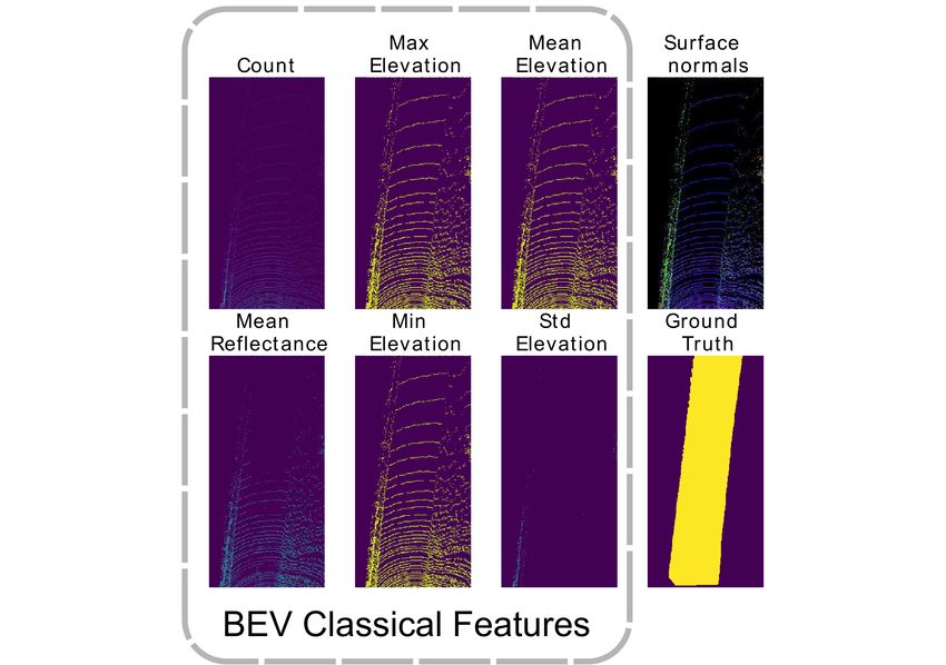
ISPRS Annals of the Photogrammetry, Remote Sensing and Spatial Information Sciences, Volume V-2-2020, 2020
                                             XXIV ISPRS Congress (2020 edition)

Figure 1. Overall methodology to evaluate the performance of road segmentation across different resolutions. See Figures 3 for more
                                                 details on the architectures used.

position of the layer in the laser stack and the value of the azi-   2.1   DNN models
muth angle. Basically, for a scanner with 64 layers we assign
the point x to a cell in row i if x has been acquired by the i-th    The LoDNN architecture from (Caltagirone et al., 2017) is a
layer starting from the top. We decided to use this approach         FCN designed for semantic segmentation, it has an input layer
because in the scanner the layers are not uniformly spaced and       that takes as input the BEV images, an encoder, a context mod-
using standard SV projection causes that different points col-       ule that performs multi-scale feature aggregation using dilated
lide on the same cell and strips of cells are empty in the final     convolutions and a decoder which returns confidence map for
image as illustrated in Fig.2. In subsection 2.2, we describe how    the road. Instead of Max unpooling layer 1 specified in (Calta-
we associate each point at the layer that captured it. However,      girone et al., 2017), we use a deconvolution layer (Zeiler et al.,
we underline that our method relies on the way the points are        2010). Other than this modification, we have followed the au-
ordered in the point cloud array.                                    thors implementation of the LoDNN. The architecture is repor-
                                                                     ted in Fig. 3a.
Finally, following (Velas et al., 2018), in each grid cell we com-
pute the minimum elevation, mean reflectivity and minimum ra-        The U-Net architecture (Ronneberger et al., 2015), is a FCN
dial distance from the scanner. This information is encoded in a     designed for semantic segmentation. In our implementation of
three-channel image. In Fig. 7, an example of the SV projection      U-Net, the architecture is made of three steps of downsampling
is shown in the first three images from the top. Since these three   and three steps of upsampling. During the downsampling part
features are already used in the state of the art for the ground     1 × 2 max pooling is used to reduce the features spatial size. In
segmentation task, in SV we refer to SV Classical Features, as       order to compare the different cases (64/32/16 scanning layers)
the set of SV images composed by minimum elevation, mean             among them, the 64 scanning layers ground truth is used for all
reflectivity and minimum radial length.                              the cases. For this purpose an additional upsampling layer of
                                                                     size 2 × 1 is required at the end of the 32-based architecture and
                       Standard Projection                           two upsampling layers at the end of the 16. In fact the size of SV
                                                                     images for the 32 scanning layer is 32 × 2048. Thus without an
                                                                     additional upsampling layer we would obtain an output image
                                                                     whose size is 32 × 2048. Similarly, for the 16 scanning layer,
                          Our Projection                             we add two upsampling layers of size 2×1 to go from 16×2048
                                                                     to 64 × 2048 pixels output images. Fig. 3b, 3c & 3d illustrate
                                                                     the three architectures used.
                                                                     In both cases a confidence map is generated by each model.
                                                                     Each pixel value specifies the probability of whether corres-
      Figure 2. SV projection: two cropped images showing            ponding grid cell of the region belongs to the road class. The
 difference between the standard projection, and our projection.     final segmentation is obtained by thresholding at 0.5 the confid-
                                                                     ence map.
Once extracted these feature maps we use them as input to train         1 In the context of DNN, a layer is a general term that applies to a
DNNs for binary segmentation. We trained LoDNN model for             collection of ’nodes’ operating together at a specific depth within a neural
the case of BEV projection, and U-Net model in the case of SV        network. In the context of LIDAR scanners, the number of scanning layer
projection.                                                          refers to the number of laser beams installed in the sensor.

         This contribution has been peer-reviewed. The double-blind peer-review was conducted on the basis of the full paper.
                     https://doi.org/10.5194/isprs-annals-V-2-2020-335-2020 | © Authors 2020. CC BY 4.0 License.                            337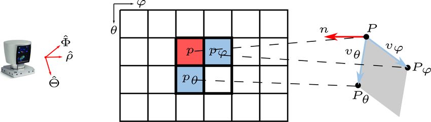
ISPRS Annals of the Photogrammetry, Remote Sensing and Spatial Information Sciences, Volume V-2-2020, 2020
XXIV ISPRS Congress (2020 edition)
100x125x128
100x125x128
100x125x128
100x125x128
100x125x128
100x125x128
100x125x128
100x125x128
200x250x32
200x250x32
100x125x32
100x125x32
200x250x32
200x250x32
200x250x32
Conv 3x3 Stride 1 Conv 1x1
Output ground BEV Map
Input Feature maps MaxPool2x2 Stride 2 Softmax
Dilated Conv 3x3 with Stride 1
Zero-padding, SpatialDropOut + ELU
(a) LoDNN Architecture by authors (Caltagirone et al., 2017) in our experiments on BEV.
6
4
4
4
2
2
2
8
48
20 8
48
25
2
2
2
51
51
51
4
4
1
10
10
10
20
20
20
32
32 Bottleneck 64 32
16 32 16
6 8 16 8
Input
PRED
h: 64
(b) U-Net architecture used for the 64 layer.
6
24
24
24
2
2
2
48
48
20 8
48
25
51
51
51
4
10
10
10
20
20
20
8
32
4
1
20
32 Bottleneck 64 32
16 32 16
6 8 16 8
Input 8
h: 32
h: 32 Up
PRED
h: 64
(c) U-Net architecture used for the 32 layer.
6
24
24
24
2
2
2
48
48
20 8
48
25
51
51
51
4
10
10
10
20
20
20
48
32
20
48
32 64 32
1
Bottleneck
20
16 32 16
6 8 16 8
Input 8
h: 16
h: 16 Up 8
h: 32 Up
PRED
h: 64
(d) U-Net architecture used for the 16 layer.
Figure 3. (a) LoDNN Architecture used on BEV images. (b-d) U-Net Architectures used on SV images.
This contribution has been peer-reviewed. The double-blind peer-review was conducted on the basis of the full paper.
https://doi.org/10.5194/isprs-annals-V-2-2020-335-2020 | © Authors 2020. CC BY 4.0 License. 338
ISPRS Annals of the Photogrammetry, Remote Sensing and Spatial Information Sciences, Volume V-2-2020, 2020
XXIV ISPRS Congress (2020 edition)
2.2 Sub-sampling point clouds to simulate low resolution
Azimuthal angles
1
0
−1
Figure 5. Relationship between adjacent pixels in the radial
0 10000 20000 30000 40000 50000 60000 distance image R and adjacent points in the 3D space. Pixels p,
Polar angles
2.0 pϕ and pθ are associated to 3D points P , Pϕ and Pθ . Since P ,
Pϕ and Pθ compose a local plane, we compute their 3D
1.8
gradients as tangent vectors vϕ , vθ from a radial distance value
1.6 at p, pϕ and pθ .
0 10000 20000 30000 40000 50000 60000
R at pixels p, pϕ as
Figure 4. Plot containing the azimuths and vertical angles for a
dϕ R(ϕ, θ) cos(ϕ) sin(θ) + R(ϕ, θ) cos(ϕ) cos(θ)
single point cloud. vϕ (ϕ, θ) = dϕ R(ϕ, θ) sin(ϕ) sin(θ) + R(ϕ, θ) sin(ϕ) cos(θ)
dϕ R(ϕ, θ) cos(θ) − R(ϕ, θ) sin(θ)
Currently there are no dataset available containing scans of the
same environment taken simultaneously with scanners at dif-
ferent resolutions, we simulated the 32 and 16 layer scans re- where
moving layers from 64 scans. To achieve this, we first need to
R(ϕ + ∆ϕ, θ) − R(ϕ, θ)
associate each point within each 64 scan to the scanning layer dϕ R(ϕ, θ) =
it was captured from. We exploit the special ordering in which ∆ϕ
(2)
point clouds have been stored within the KITTI datasets. Fig. R(pϕ ) − R(p) ∂R
= ≈ (ϕ, θ).
4 shows the azimuth and polar angles of the sequence of points ∆ϕ ∂ϕ
of a single scan. We observe that the azimuth curve contains
64 cycles over 2π degrees, while polar curve globally increase.
Similarly vθ is obtained using values at p and pθ as:
Thus a layer corresponds to a round of 2π degrees in the vector
of azimuths. Scanning layers are stored one after another start-
dθ R(ϕ, θ) cos(ϕ) sin(θ) − R(ϕ, θ) sin(ϕ) sin(θ)
ing from the uppermost layer to the lowermost one. As we step
vθ (ϕ, θ) = dθ R(ϕ, θ) sin(ϕ) sin(θ) + R(ϕ, θ) cos(ϕ) sin(θ)
through sequentially 2π in the azimuth angle (two zero cross-
dθ R(ϕ, θ) cos(θ)
ings), we label each point to be within the same layer. Once re-
trieved the layers, we can obtain a 32 scan removing one layer
where
out of two from the 64 scan, and obtain a 16 scan removing
three layers out of four. The size of SV input images changes R(ϕ, θ + ∆θ) − R(ϕ, θ)
when we remove layers. We move from 64 × 2048 pixels for dθ R(ϕ, θ) =
∆θ (3)
a 64 layer scanner to 32 × 2048 pixels for the 32 layer and to R(pθ ) − R(p) ∂R
16 × 2048 pixels for the 16 layer. = ≈ (ϕ, θ).
∆θ ∂θ
2.3 Surface normal extraction The approximated normal vector is n = vϕ × vθ . Once the sur-
face point normals are estimated in the SV, we get them back to
3D-cartesian coordinates, and subsequently project them onto
Along with features used in the state of the art, we estimate sur- the BEV. This adds three supplementary channels to the input
face normals from the image containing radial distances in the images. Fig. 7 shows the results obtained on SV image with
SV. Our method is inspired by the work of (Nakagawa et al., 64 layer. For each pixel we mapped the coordinates (x, y, z)
2015) where the authors estimate surface normals using depth of the estimated normals to the RGB color map, so x → R,
image gradients. Let p = (ϕ, θ) a couple of angles in the spher- y → G and z → B . Please remark that a FCN can not extract
ical grid and let R be the image containing the radial distances. this kind of features through convolutional layers starting from
We can associate to p a point P in the 3D space using the for- SV classic features. In fact, to extract this kind of information
mula using convolution the FCN should be aware of the position of
the pixel inside of the image, i.e. know the angles (ϕ, θ), but
x = R(ϕ, θ) cos(ϕ) sin(θ),
this would break the translational symmetry of convolutions.
Ψ(ϕ, θ) = y = R(ϕ, θ) sin(ϕ) sin(θ), (1) This enforces prior geometrical information to be encoded in
z = R(ϕ, θ) cos(θ). the features maps that are the input of the DNN. Finally, we
also remark that the normal feature maps are computationally
efficient since its a purely local operation in the spherical co-
Now, let pϕ = (ϕ + ∆ϕ, θ) and pθ = (ϕ, θ + ∆θ) respectively
ordinates.
the vertical and the horizontal neighbouring cells. They have
two corresponding points Pϕ and Pθ in the 3D space, as well.
Since P , Pϕ and Pθ compose a local 3D plane, we can estimate 3. EXPERIMENTS & ANALYSIS
the normal vector ∂Ψ
∂ϕ
× ∂Ψ
∂ϕ
at P using the two vectors vϕ , vθ
spanning the local surface containing P , Pϕ and Pθ , as in Fig. The binary road segmentation task is evaluated on two datas-
5. We compute vϕ using the values of the radial distance image sets : 1. the KITTI road segmentation (Fritsch et al., 2013),
This contribution has been peer-reviewed. The double-blind peer-review was conducted on the basis of the full paper.
https://doi.org/10.5194/isprs-annals-V-2-2020-335-2020 | © Authors 2020. CC BY 4.0 License. 339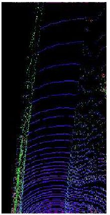
ISPRS Annals of the Photogrammetry, Remote Sensing and Spatial Information Sciences, Volume V-2-2020, 2020
                                             XXIV ISPRS Congress (2020 edition)

                                                                     Training : Adam optimiser with initial learning rate of 0.0001
                       Max                 Mean        Surface       is used to train the models. The models were trained using an
      Count          Elevat ion           Elevat ion   norm als      Early-Stopping. We used the Focal loss with gamma factor of
                                                                     γ = 2 (Lin et al., 2017), thus the resulting loss is L(pt ) =
                                                                     −(1 − pt )γ log(pt ), where
                                                                                                (
                                                                                                    p     if y = 1,
                                                                                         pt =
                                                                                                    1−p   otherwise.

                                                                     The focal loss was useful in the KITTI Road segmentation
                                                                     benchmark. The road class was measured to be around 35%
     Mean              Min                  St d       Ground
   Reflect ance      Elevat ion           Elevat ion    Trut h
                                                                     of the train and validation set, in the BEV, while around 5% for
                                                                     the SV. This drastic drop in the road class in SV is due to the
                                                                     restriction of the labels to the camera FOV. While for Semantic-
                                                                     KITTI we observed lesser level of imbalance between road and
                                                                     background classes.

                                                                     Metrics : We use the following scores to benchmark our ex-
                                                                     periments. The F1 -Score and Average Precision are defined
                                                                     as

                                                                                        P ∗R        X
                                                                             F1 = 2 ∗        , AP =   Pn (Rn − Rn−1 )                 (4)
                                                                                        P +R
                                                                                                           n

 Figure 6. An example of features projected on the BEV in case
of a 64 layers scanner. Surface normals are computed on SV and       where, P = T PT+F  P
                                                                                          P
                                                                                             R = T PT+F P
                                                                                                           N
                                                                                                              and Pn , Rn are precision
                        projected to BEV.                            and recall at n-th threshold. In all the cases the scores have been
                                                                     measured on the projected images, and we report them in Table
                                                                     2.
                          Radial Dist ance
                                                                     Evaluating different resolutions: When subsampling point
                                                                     clouds, the input SV image size changes accordingly. For ex-
                            Reflect ance                             ample, after the first subsampling the input SV image now has a
                                                                     size of 32×2048. In order to get fair comparison, the evaluation
                                                                     of all results is made at the original full resolution at 64 × 2048.
                             Elevat ion
                                                                     In such as case the number of layers in the U-Net architectures
                                                                     has been increased to up-sample the output segmentation map
                                                                     to the full resolution. This lead to 3 different architectures for
                    Est im at ed surface norm als
                                                                     16, 32 and 64 layers, see Fig. 3b, 3c & 3d. Three different mod-
                                                                     els were trained on the different SV images. In the Semantic
                           Ground Trut h
                                                                     KITTI dataset the evaluation has been done over the road class.
                                                                     The BEV image on the other hand remains the same size with
                                                                     subsampling. Though subsampling in BEV introduces more
                                                                     empty cells as certain layers disappear.

Figure 7. A crop example of features projected on the SV in case     3.1   KITTI road estimation benchmark
   of a 64 layers scanner. Surface normals are estimated from
 radial distance image. The last image below is the ground truth     The KITTI road segmentation dataset consists of three categor-
                           for this case.                            ies: urban unmarked (UU),urban marked (UM), and urban mul-
                                                                     tiple marked lanes (UMM). Since the test dataset’s ground truth
                                                                     is not publicly available, 289 training samples from the dataset
2. Semantic-KITTI dataset (Behley et al., 2019). The input           is split into training, validation and test sets for the experiments.
information to the DNNs comes purely from point clouds and           Validation and test sets have 30 samples each and the remaining
no camera image information was used. The BEV and SV rep-            229 samples are taken as training set.
resentations were used over the point clouds from KITTI road-
dataset, while only the SV representation over Semantic-KITTI.       Ground truth annotations are represented only within the cam-
The BEV ground truth information for semantic-KITTI did not          era perspective for the training set. We use the ground truth an-
currently exist during the redaction of this article, and thus no    notations provided by authors (Caltagirone et al., 2017) in our
evaluation was performed. The projection of the 3D labels to         experiments. The BEV groudtruth was generated over the xy-
BEV image in semantic-KITTI produced sparsely labeled BEV            grid within [−10, 10] × [6, 46] with squares of size 0.10 × 0.10
images and not a dense ground truth as compared the BEV              meters.
ground truth in Fig. 6. The SV ground truth images have been
generated by projecting 3D labels to 2D pixels. We consider a        Figures 8, 9 illustrate the Precision-Recall (PR) curves obtained
pixel as road if at least one road 3D point is projected on the      on BEV images and SV images. The performance metrics
pixel.                                                               for the different resolutions (64/32/16 scanning layers) of the

         This contribution has been peer-reviewed. The double-blind peer-review was conducted on the basis of the full paper.
                     https://doi.org/10.5194/isprs-annals-V-2-2020-335-2020 | © Authors 2020. CC BY 4.0 License.                      340
ISPRS Annals of the Photogrammetry, Remote Sensing and Spatial Information Sciences, Volume V-2-2020, 2020
XXIV ISPRS Congress (2020 edition)
scanners are reported, for both the classical and classical-with- KITTI Road-Seg, BEV AP F1 Rec Prec
normal features. At full resolution the classic features obtain Classical (64) 0.981 0.932 0.944 0.920
state of the art scores as reported by authors (Caltagirone et al., Classical + Normals (64) 0.983 0.935 0.945 0.926
Classical (32) 0.979 0.920 0.926 0.914
2017). In Table 2, we observe that with subsampling and re- Classical + Normals (32) 0.984 0.934 0.937 0.930
duction in the number of layers, there is a degradation in the AP Classical (16) 0.978 0.918 0.920 0.915
along with metrics. With the addition of the normal features, we Classical + Normals (16) 0.981 0.927 0.936 0.919
observe and improvement in AP across all resolutions/number KITTI Road-Seg, SV AP F1 Rec Prec
of layers. Classical (64) 0.960 0.889 0.914 0.889
Classical + Normals (64) 0.981 0.927 0.926 0.929
1.000
BEV - Precision Recall Curve Classical (32) 0.965 0.896 0.915 0.878
Classical + Normals (32) 0.981 0.927 0.928 0.927
Classical (16) 0.960 0.888 0.900 0.875
0.975 Classical + Normals (16) 0.974 0.906 0.914 0.899
0.950
Table 2. Results obtained on the test set of the KITTI road
segmentation dataset in the BEV and SV.
0.925
metry dataset, for various road scene objects, road, vegeation,
sidewalk and other classes. The dataset was split into train and
Precision
0.900 test datasets considering only the road class. To reduce the
size of the dataset, and temporal correlation between frames,
0.875
we sampled one in every ten frames over the sequences 01-10
excluding the sequence 08, over which we reported the our per-
formance scores. The split between training and test has been
0.850 done following directives in (Behley et al., 2019).
Classic
Classic + Normals
0.825 Classic (32) With the decrease in vertical angular resolution by subsampling
Classic + Normals (32) the original 64 layer SV image we observe a minor but defin-
Classic (16)
Classic + Normals (16) ite drop in the binary road segmentation performance (in vari-
0.800 ous metrics) for sparse point clouds with 32 and 16 scanning
0.800 0.825 0.850 0.875 0.900 0.925 0.950 0.975 1.000
Recall layers. This is decrease is visible both in Table 3 but also in
the Precision-Recall curve in Fig. 10. With the addition of
Figure 8. KITTI Road Segmentation with BEV images: our normal features to the classical features we do observe a
Precision-Recall Curve for various features with and without clear improvement in performance across all resolutions (16,
sub-sampling. 32 and 64 scanning layers). Geometrical normal features chan-
Spherical View - Precision Recall Curve nel as demonstrated in Fig. 7 show their high correlation w.r.t
1.000
the road class region in the ground-truth. Road and ground re-
gions represent demonstrate surfaces which are low elevation
0.975 flat surfaces with normal’s homogeneously pointing in the same
directions.
0.950 Semantic KITTI-SV AP F1 Rec Prec
Classical (64) 0.969 0.907 0.900 0.914
Classical + Normals (64) 0.981 0.927 0.927 0.927
0.925
Classical (32) 0.958 0.897 0.902 0.892
Classical + Normals (32) 0.962 0.906 0.906 0.906
Precision
0.900
Classical (16) 0.944 0.880 0.879 0.882
Classical + Normals (16) 0.948 0.889 0.894 0.883
0.875 Table 3. Results obtained on the test set of the Semantic-KITTI
dataset in the SV.
0.850
Classic
Classic + Normals 4. CONCLUSION
0.825 Classic (32)
Classic + Normals (32)
Classic (16) In view of evaluating the performance of low-resolution LID-
Classic + Normals (16)
0.800
ARs for segmentation of the road class, in this study we eval-
0.800 0.825 0.850 0.875 0.900 0.925 0.950 0.975 1.000
Recall uate the effect of subsampled LIDAR point clouds on the per-
formance of prediction. This is to simulate the evaluation of low
Figure 9. KITTI Road Segmentation with SV images: resolution scanners for the task of road segmentation. As expec-
Precision-Recall Curve for various features with and without ted, reducing the point cloud resolution reduces the segmenta-
sub-sampling. tion performances. Given the intrinsic horizontal nature of the
road we propose to use estimated surface normals. These fea-
3.2 Semantic-KITTI tures cannot be obtained by a FCN using Classical Features as
input. We demonstrate that the use of normal features increase
The Semantic-KITTI dataset is a recent dataset that provides a the performance across all resolutions and mitigate the deteri-
pointwise label across the different sequences from KITTI Odo- oration in performance of road detection due to subsampling in
This contribution has been peer-reviewed. The double-blind peer-review was conducted on the basis of the full paper.
https://doi.org/10.5194/isprs-annals-V-2-2020-335-2020 | © Authors 2020. CC BY 4.0 License. 341ISPRS Annals of the Photogrammetry, Remote Sensing and Spatial Information Sciences, Volume V-2-2020, 2020
XXIV ISPRS Congress (2020 edition)
1.000
SemanticKITTI - SV - Precision Recall Curve Caltagirone, L., Scheidegger, S., Svensson, L., Wahde, M.,
2017. Fast lidar-based road detection using fully convolutional
neural networks. 2017 ieee intelligent vehicles symposium (iv),
0.975
IEEE, 1019–1024.
0.950
Chen, L., Yang, J., Kong, H., 2017. Lidar-histogram for fast
road and obstacle detection. 2017 IEEE International Confer-
ence on Robotics and Automation (ICRA), IEEE, 1343–1348.
0.925
del Pino, I., Vaquero, V., Masini, B., Solà, J., Moreno-Noguer,
Precision
F., Sanfeliu, A., Andrade-Cetto, J., 2017. Low resolution lidar-
0.900
based multi-object tracking for driving applications. Iberian
Robotics conference, Springer, 287–298.
0.875
Fritsch, J., Kuehnl, T., Geiger, A., 2013. A new perform-
ance measure and evaluation benchmark for road detection al-
0.850
gorithms. International Conference on Intelligent Transporta-
Classic
Classic + Normals tion Systems (ITSC).
0.825
Classic (32)
Classic + Normals (32) Jaritz, M., De Charette, R., Wirbel, E., Perrotton, X.,
Classic (16)
Classic + Normals (16) Nashashibi, F., 2018. Sparse and dense data with cnns: Depth
0.800
0.800 0.825 0.850 0.875 0.900 0.925 0.950 0.975 1.000 completion and semantic segmentation. 2018 International
Recall
Conference on 3D Vision (3DV), IEEE, 52–60.
Figure 10. SemanticKITTI with SV images: Precision-Recall Lin, T.-Y., Goyal, P., Girshick, R., He, K., Dollár, P., 2017.
Curve for various features with and without sub-sampling. Focal loss for dense object detection. Proceedings of the IEEE
international conference on computer vision, 2980–2988.
both BEV and SV. Normals features encode planarity of roads
and is robust to subsampling. Lyu, Y., Bai, L., Huang, X., 2018. Chipnet: Real-time lidar
processing for drivable region segmentation on an fpga. IEEE
Transactions on Circuits and Systems I: Regular Papers, 66(5),
4.1 Future work 1769–1779.
In future works we aim to study the effect of temporal aggreg- Milioto, A., Stachniss, C., 2019. Rangenet++: Fast and accurate
ation of LIDAR scans on reduced spatial resolution due to sub- lidar semantic segmentation. Proc. of the IEEE/RSJ Intl. Conf.
sampling the vertical angle. Furthermore, in SV we upsampled on Intelligent Robots and Systems (IROS).
the information inside the network, just before the prediction
layer. In future works we would like to upsample the input Nakagawa, Y., Uchiyama, H., Nagahara, H., Taniguchi, R.-I.,
SV range images, and evaluate the performance of the U-Net 2015. Estimating surface normals with depth image gradients
model on the original 64 × 2048 sized SV range image. The for fast and accurate registration. 3D Vision (3DV), 2015 Inter-
up-sampling can be trained end-to-end to achieve successful re- national Conference on, IEEE, 640–647.
construction of 64 × 2048 image from sub-sampled 32 × 2048 Ronneberger, O., Fischer, P., Brox, T., 2015. U-net: Convo-
or 16 × 2048 images. lutional networks for biomedical image segmentation. Interna-
tional Conference on Medical image computing and computer-
We have focused our study on road segmentation mainly to limit assisted intervention, Springer, 234–241.
and understand the effect of subsampling on a geometrically
simple case. In our future study we aim to evaluate performance Roynard, X., Deschaud, J.-E., Goulette, F., 2018. Paris-Lille-
of key classes i.e. cars, pedestrians, to determine the loss in 3D: A large and high-quality ground-truth urban point cloud
accuracy on account of subsampling of pointclouds. dataset for automatic segmentation and classification. The In-
ternational Journal of Robotics Research, 37(6), 545-557.
ACKNOWLEDGEMENTS Serna, A., Marcotegui, B., 2014. Detection, segmentation and
classification of 3D urban objects using mathematical morpho-
logy and supervised learning. ISPRS Journal of Photogram-
We thank authors of LoDNN for their insights and support.
metry and Remote Sensing, 93, 243–255.
Velas, M., Spanel, M., Hradis, M., Herout, A., 2018. Cnn for
REFERENCES
very fast ground segmentation in velodyne lidar data. 2018
IEEE International Conference on Autonomous Robot Systems
Behley, J., Garbade, M., Milioto, A., Quenzel, J., Behnke, S., and Competitions (ICARSC), IEEE, 97–103.
Stachniss, C., Gall, J., 2019. SemanticKITTI: A Dataset for Se-
mantic Scene Understanding of LiDAR Sequences. Proc. of the Velodyne LiDAR, Wikipedia, n.d. https://en.wikipedia.
IEEE/CVF International Conf. on Computer Vision (ICCV). org/wiki/Velodyne_LiDAR. Accessed: 27 Jan 2019.
Zeiler, M. D., Krishnan, D., Taylor, G. W., Fergus, R., 2010.
Caesar, H., Bankiti, V., Lang, A. H., Vora, S., Liong, V. E.,
Deconvolutional networks. 2010 IEEE Computer Society Con-
Xu, Q., Krishnan, A., Pan, Y., Baldan, G., Beijbom, O., 2019.
ference on computer vision and pattern recognition, IEEE,
nuScenes: A multimodal dataset for autonomous driving. arXiv
2528–2535.
preprint arXiv:1903.11027.
This contribution has been peer-reviewed. The double-blind peer-review was conducted on the basis of the full paper.
https://doi.org/10.5194/isprs-annals-V-2-2020-335-2020 | © Authors 2020. CC BY 4.0 License. 342You can also read