Satellite Image Building Detection using U-Net Convolutional Neural Network
←
→
Page content transcription
If your browser does not render page correctly, please read the page content below
EE 5561 IMAGE PROCESSING AND APPLICATIONS, SPRING 2021                                                                              1

      Satellite Image Building Detection using U-Net
                Convolutional Neural Network
                                 Liam Coulter, Teague Hall, Luis Guzman, Isaac Kasahara

   Abstract—Convolutional Neural Networks (CNNs) are at the           presence and location of buildings. The objective is to au-
forefront of current image processing work in segmentation            tomatically generate a set of building polygons that most
and object detection. We apply a U-Net CNN architecture to            closely approximates the manually generated polygons. In
a satellite imagery data set to detect building instances in birds-
eye view image patches, since the U-Net has been shown to             order to assess the quality of automatically generated building
achieve high accuracy with low complexity and training time.          polygons or masks, SpaceNet uses several metrics including
We present our results in the context of the SpaceNet Building        the Intersection over Union (IoU), precision, recall, and F1
Detection v1 Challenge, and compare scores against the winning        scores described in the next section. Subsequent SpaceNet
algorithms. Results from our implementation demonstrate the           challenges focused on extracting other features from satellite
U-Net architecture’s ability to successfully detect buildings from
satellite images. We discuss the challenges and limitations of        imagery such as roadways (challenges 3 and 5), generat-
using CNNs and the U-Net in particular for image segmentation,        ing building detections from other types of data including
despite the success of our implementation.                            Synthetic Aperture Radar/SAR (challenges 4 and 6), and
                                                                      making high-level inferences about route transit time or urban
                                                                      development (challenges 5 and 7). We focus only on building
                       I. I NTRODUCTION                               detection here.
                                                                         Our project solves the SpaceNet Building Detection v1

T     HE availability of high-resolution satellite imagery has
      motivated attempts at automatically generating civil fea-
ture map systems. These maps should contain information
                                                                      challenge by using a U-Net Convolution Neural Network
                                                                      (CNN) architecture for semantic segmentation. The U-Net
                                                                      architecture was designed for biomedical image segmentation
about man-made structures such as buildings and roadways              and shows a high degree of accuracy with low complexity
which can then be used for applications in civil planning, hu-        and low training time. In addition, the U-Net employs “skip
manitarian response efforts, and more. An automated approach          connections” instead of fully connected layers, which allows
for generating these feature maps is a cheaper, faster, and           it to preserve finer details in the final segmentation map. We
potentially more accurate alternative to manual map creation.         discuss these more in detail later.
In addition, an automated approach reduces the cost and effort           The field of image segmentation has been active in recent
to update feature maps, as old manual map systems become              years, aided by advancements in machine learning methods.
outdated. This could be very valuable for geographic regions          Application areas range from biomedical imaging (for which
experiencing fast population growth, or for updating maps             the U-Net was developed) to autonomous vehicles. Semantic
after natural disasters.                                              segmentation differs from instance segmentation in that we
   SpaceNet is an open innovation project hosting freely              do not care about separating instances of the same class in
available image data with training labels for machine learning        the final segmentation map, but rather assigning a class to
and computer vision researchers. The aim of SpaceNet is to            each pixel in the image. For example, a semantic segmentation
aid advancements in the field by offering high quality la-            task would be to classify every pixel in an image as either
beled training and testing data, and corresponding challenges.        a building or not a building; an instance segmentation task
Historically, satellite image data was privately managed or           would be to distinguish separate occurrences of buildings in
government controlled, making it difficult or impossible for          an image, and represent that in the final segmentation map [2].
researchers to use for algorithm development. SpaceNet has            The current state-of-the-art in semantic segmentation consists
compiled extensive image sets along with labeled training data        mainly of machine learning methods since the development
which is made free to the public in the hope of advancing             of AlexNet [3], specifically CNNs and U-Net variants, since
automated algorithms. The majority of activity in these algo-         fully connected CNNs tend to have trouble with fine details.
rithms has been dominated by machine learning approaches.             Two recent U-Net variants confirm this difficulty, underscoring
In addition to providing free data sets, SpaceNet organizes           the importance of using skip connections instead of fully
targeted competitions that look at specific sub-problems within       connected layers [4], [5].
satellite image mapping. These competitions intend to motivate           This report is organized as follows. Section II provides a
interest and advancements in the topic.                               description of the SpaceNet Building Detection v1 challenge,
   The first SpaceNet challenge (“Building Detection v1”)             with discussion of data, labels, solution requirements, and
focuses on building detection from optical and hyperspectral          evaluation metrics, as well as a detailed description of the
images. This challenge provides 3-band and 8-band satellite           U-Net architecture and our specific implementation including
images along with bounding polygon vertices denoting the              points of difficulty in our implementation and training. We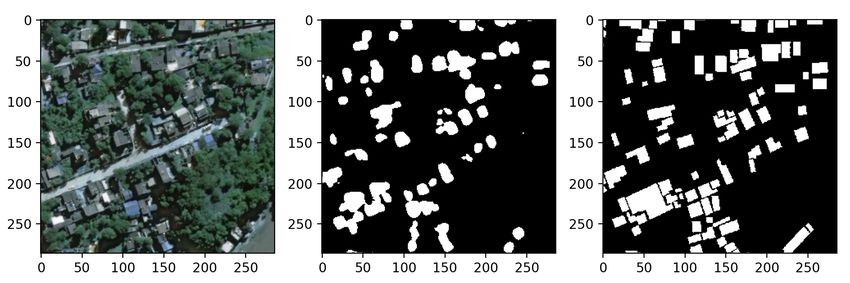
EE 5561 IMAGE PROCESSING AND APPLICATIONS, SPRING 2021                                                                            2

Fig. 1: Rio de Janeiro image tile with building polygons superimposed (left) and associated building label polygons (right)
[1]. Building polygons have varied shapes.

also describe our implemented evaluation metrics, and how          and 20% for validation, and report our accuracy numbers from
they may differ from those used by actual contestants in the       the validation set, which was not used for training. Figure
Building Detection v1 challenge. In section III we present         1 shows a single image tile along with the corresponding
the results from our U-Net implementation, and compare             building label polygons.
them to the winning results from the SpaceNet Building
Detection v1 challenge. Section IV contains a discussion of the    B. SpaceNet Evaluation Metrics
strengths and weaknesses of our approach, and a discussion
                                                                      The SpaceNet challenges use several metrics to assess
of the limitations of the U-Net architecture. Finally, we draw
                                                                   building prediction quality: Intersection over Union (IoU),
conclusions from our experimentation and analysis in section
                                                                   precision, recall, and F1 score. The precision, recall, and
V.
                                                                   F1 metrics are based on the IoU for individual buildings
                                                                   in an image, and can be computed for an individual image
                 II. M ETHODS AND T HEORY                          or across several images as a weighted average. IoU is a
                                                                   measure of how well predicted building label polygons or
A. The SpaceNet Building Detection v1 Data
                                                                   masks overlap with ground truth polygons, and is commonly
   The SpaceNet Building Detection challenge v1 data was           used to assess semantic segmentation results. Let A and B
collected from the WorldView-2 satellite and covers a 2544         be two sets of points; in our application, A represents the set
square kilometer region centered over Rio De Janerio with          of pixel locations contained within the bounds of the ground
50cm resolution [1]. The dataset is broken into individual im-     truth building label polygon and B represents the set of pixel
ages with size 200m×200m. These image “tiles” are between          locations contained within the bounds of a predicted building
438 and 439 pixels wide and between 406 and 407 pixels             location polygon or mask. The IoU then, is
tall, and the 3-band RGB images have been pan-sharpened.
                                                                                                      |A ∩ B|
The training data set consists of approximately 6000 such                              IoU (A, B) =                             (1)
3-band RGB image tiles. Along with the processed images,                                              |A ∪ B|
SpaceNet provides building labels in the form of sets of           where | · | represents set cardinality. It is apparent that IoU
polygon vertices denoting the corners of buildings in each         is shift-invariant, and independent of the size of given sets A
image. These building label polygons were generated using          and B, since the union normalizes the IoU result to within
rough automated techniques and then detailed by hand. This         the interval [0, 1]. A perfect IoU score of 1 happens when
labor intensive process resulted in approximately 380,000          a predicted building label polygon exactly coincides with the
buildings for the entire Rio de Janeiro geographic area, over      ground truth label polygon, and an IoU score of 0 occurs when
the 6000+ image tiles. The building labels polygon data are        there is no overlap at all. The IoU metric can be limiting for
provided in geoJSON files which correspond to each image           small objects where low pixel resolution can greatly influence
tile. In the original SpaceNet Building Detection v1 challenge,    the result. Further, the IoU doesn’t account for the shape of
participants used this entire labeled data set for training        predictions relative to ground truth polygons; as long as the
and validation, and submitted geoJSON files with proposed          size of the intersection and union are the same, we could have
building detections from images in a separate unlabeled testing    any number of (incorrect) predicted building shapes, and any
data set. However, since we do not have access to labels for the   sort of overlap, and the IoU would give the same score. Finally,
testing set and thus are unable to determine our performance       the IoU doesn’t account for building instances where there
from this set, we use the labeled training data set for both       is a complete mismatch between the predicted and ground
training and validation. We employ a split of 80% for training     truth polygons; the predicted polygon could be very close (but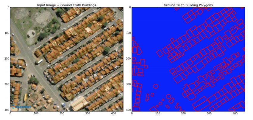
EE 5561 IMAGE PROCESSING AND APPLICATIONS, SPRING 2021 3
not intersecting) the ground truth polygon, or the predicted incorrect. Precision alone is not sufficient to assess prediction
polygon could not exist. In either case though, the IoU would quality because it is unaffected when the algorithm fails to
give a score of zero. So, the IoU by itself does not give a detect buildings. Recall, then, is the fraction of true building
complete picture of the quality of prediction results. polygons that are detected by the algorithm. That is,
To generate an overall evaluation metric for an entire image |True Positives|
or group of images, it is necessary to combine the results Recall = (3)
|True Positives| + |False Negatives|
of each IoU. This is achieved by first establishing an IoU
detection threshold of 0.5; any individual IoU result greater |True Positives|
= (4)
than this threshold is considered a successful detection. For |Ground Truth Polygons|
example, if there is one building in an image and the IoU Recall conveys information about the algorithms ability to
score is 0.4, we do not report a building detection since the detect all objects in the image and thus gives a lower score
score is below the threshold. In the case where there are several when objects are missed.
buildings in an image, we search over all predicted building To give an overall picture of the quality of a given predic-
polygons for each ground truth polygon and compute the tion, we combine the precision and recall into the F1 score:
IoU score between the current ground truth and all predicted 2 · Precision · Recall
polygons. The largest IoU is chosen as the correct match F1 = (5)
(Precision + Recall)
for the current ground truth building, and we check against
the threshold to see if the current prediction constitutes a Since precision and recall range from 0 to 1, so does F1; the
detection. If we have a detection, we say we have found a true 2 in the numerator serves as a normalizing factor.
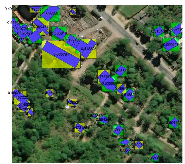
positive, and if not we say we have found a false positive. We Figure 3 shows an example image with predictions and
then remove the current predicted and ground truth polygons ground truth polygons. The ground truth polygons are shown
from the list, and move on to the next ground truth polygon in blue, and predictions are either green or yellow, signifying
(cycling through all remaining predicted polygons again). This an IoU score above or below 0.5, respectively.
process is shown in figure 2.
Fig. 3: Performance evaluation of image tile using IoU [6].
Fig. 2: Assessing predicted building polygons using IoU [6].
C. Image Pre-Processing
Once we have determined the number of true positives, false Since SpaceNet data was in the form of TIFF images
positives, and false negatives (where we have a ground truth and corresponding geoJSON building polygon labels, we had
building but no predicted building polygon), we define the to convert these to a format that was easier to work with
precision and recall. Precision is defined as the number of in the context of training a CNN. We made use of the
true positive predicted building detections divided by the total publicly-available SpaceNet utilities [7] to convert the building
number of predicted buildings. That is, polygons in the geoJSON files from latitude and longitude to
image coordinates in pixels, and save the result as a binary
|True Positives|
Precision = (2) image mask with 0 denoting that there is no building in that
|Total Predicted Buildings| pixel location and 1 denoting the existence of a building.
This metric conveys information on the algorithm’s ability In order to make use of the IoU metric, we had to be able
to detect buildings while avoiding false detections; a higher to identify how many building mask polygons existed in both
precision means more detections are correct, and fewer are the ground truth and predicted building masks. For this we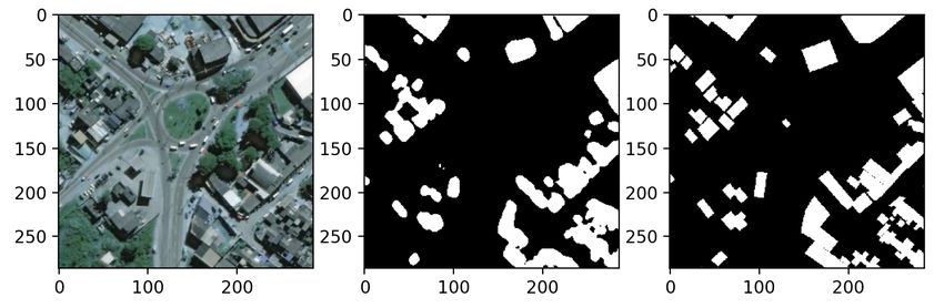
EE 5561 IMAGE PROCESSING AND APPLICATIONS, SPRING 2021                                                                                 4

                                                                      by a rectified linear unit (ReLU) activation function, defined
                                                                      by
                                                                                          ReLU(x) = max{0, x}                       (6)
                                                                      to give an activation map. Then, a 2×2 max pooling operation
                                                                      is applied with a stride length of 2 in order to downsample
                                                                      the signal to a still smaller size. The 2 × 2 max pooling
                                                                      operation involves taking the max of each 2 × 2 patch of the
                                                                      signal, as a way of downsampling the signal while keeping
       (a) Building Mask               (b) Building Contours          the elements with the largest activation result. At each level
                                                                      of the contraction path, the feature channels are doubled.
Fig. 4: Building mask          and   resulting   polygons      from   At the base of the U we have our most contracted signal
cv2.findContours.
                                                                      feature map, with dimension 1024×30×30, meaning we have
                                                                      1024 feature channels. The intuition behind feature channel
                                                                      doubling is to allow the network to build more complex
used the openCV function findContours on the image                    features in subsequent layers. Since the feature channels of
masks, which returns a list of objects with polygon corners           the previous layers act as primitives for the construction of
in pixel coordinates for each polygon in the image. Figure 7          new features, doubling the number of channels allows for a
shows the building mask and result of cv2.findContours.               balance between quantity and semantic meaning of the learned
One possible discrepancy between this and the polygons in the         features.
geoJSON files is that collections of buildings which are very            The right side of the U-net is an expansive path where each
close together may appear in the building mask as one long            level involves up-convolving the feature channels followed
building. Since we used the same image masks for training             by two 3 × 3 convolutions and ReLU. Up-convolution is
and this occurrence was not very frequent, we decided this            an upsampling technique where a learned convolution mask
was an issue we did not need to address.                              is multiplied by each cell of the spatially lower-resolution
   Finally, we normalized the RGB images to [0, 1] for numeri-        signal in order to obtain a higher-resolution signal. This differs
cal stability when training our U-Net. We also standardized the       from traditional up-sampling where an unlearned mapping is
size of the images by removing a column and/or row where              used to increase signal resolution. Additionally, each level
necessary so that all images had size 406 × 438, and then             of the expansion path is concatenated with its corresponding
resized the images to 286 × 286.                                      contraction level feature map, which is cropped to match the
                                                                      size of the expansion feature vector. This allows the U-net to
                                                                      maintain spatially localized information that would otherwise
D. U-Net CNN Architecture                                             be lost during contraction. Each level of the expansion path
                                                                      halves the number of feature channels while increasing the
   Our building detector is based on the U-Net CNN architec-
                                                                      spatial resolution of the signal.
ture. This architecture was originally developed for biomedical
                                                                         The channels of the output signal will correspond to the
image segmentation, to distinguish cells in an image [8]. Since
                                                                      desired number of segmentation classes, in our case one. This
then, this architecture has been applied many times to image
                                                                      is achieved by a final 1 × 1 convolution layer that maps
segmentation problems in a variety of applications, and shows
                                                                      the output to the desired number of classes. The architecture
robustness and accuracy without long training times or high
                                                                      illustrated in figure 5 corresponds to a two class segmentation
complexity. Thus, it is an appropriate method for our building
                                                                      problem, and hence has an output depth of two.
detection problem.
                                                                         The U-net architecture is trained using the satellite images
   The U-Net architecture gets its name from the contrac-             and associated segmentation maps (binary building masks),
tion and subsequent expansion of feature maps, conceptually           using a cross-entropy loss function. The original method
shown as a U shape as in figure 5. The contraction or encoding        proposed in [8] features a pixel-wise softmax over the output
path compacts the input image signal to a map of feature              feature map combined with a cross entropy loss function. The
channels, and the expansion or decoding path then generates           softmax is defined pixel-wise as
a segmentation mask through up-convolution, which reduces
the number of feature channels at each step. This expansion
path operates in a feed-forward manner.                                                                eak (x)
                                                                                           pk (x) =   K
                                                                                                                                    (7)
   Figure 5 shows the U-Net architecture for a 512 × 512                                              X
input image. The contraction path resembles a typical CNN                                                eak0 (x)
                                                                                                      k0 =1
architecture found in many machine learning applications
where the image is compacted to a feature map representation          where ak (x) is the activation in feature channel k at pixel
with additional channels, termed feature channels. At each            location x, pk (x) is the new value of the pixel in feature
level of the contracting path, the signal undergoes a set of          channel k at location x, and K is the total number of feature
two 3 × 3 convolution operations which reduce the signal size         channels. We then combine this soft-max function with a
if padding is not used. Each convolution operation is followed        cross-entropy penalty defined over the pixel region Ω as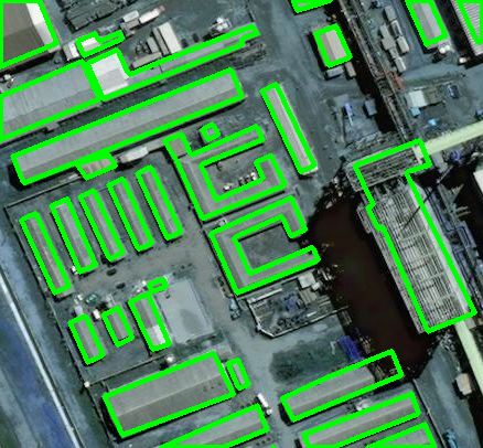
EE 5561 IMAGE PROCESSING AND APPLICATIONS, SPRING 2021                                                                               5

                                  Fig. 5: U-Net CNN architecture for 512 × 512 input images [8].

                                                                      to choose initial weights where each feature map has unit
                         X                                            variance. For the U-Net architecture then, weights should be
                 E=−           pl(x) (x) log (p(x))            (8)    drawn from a p  zero-mean normal distribution with standard
                         x∈Ω
                                                                      deviation σ = 2/N where N indicates the number of input
where l(x) is the true label of the pixel at location x, pl(x) (x)    nodes for each neuron.
is the true probability distribution of each class, and p(x) is
the estimated distribution.                                           E. U-Net Implementation
   The original U-Net paper used a slightly different loss
function aimed at improving performance of border pixels,                We implemented our U-Net using PyTorch. Following the
defined as                                                            architecture just discussed, our U-Net had 5 encoding levels
                          X                                          and 4 decoding levels (plus the final 1 × 1 convolution), and
              Eweighted =      w(x) log pl(x) (x)              (9)    output a final binary segmentation map.
                          x∈Ω                                            In order to load the images and building masks, we im-
with                                                                  plemented a custom data loader using PyTorch that would
                                                                      standardize the image and mask sizes by removing a row or
                                (d1 (x) + d2 (x))2

       w(x) = wc (x) + w0 exp −                               (10)    column where necessary, and reduced image sizes to 286×286,
                                       2σ 2                           half that used in [8] as previously discussed. This size was
where wc is a pre-computed weight map intended to balance             chosen to speed up the training process and to avoid stability
segmentation class frequencies, d1 (x) is the distance from x         issues we encountered when training on larger images. We also
to the neared object border, and d2 (x) is the distance from x        normalized the RGB images to [0, 1]. As mentioned above, we
to the border of the second closest object. The parameters w0         used the SpaceNet Building Detection v1 training data for both
and σ can be chosen manually.                                         training and validation/testing. In our data loader we used 80%
   The weight function w(x) is predefined by the ground               of the data for training, and 20% for validation/testing.
truth segmentation mask, and is used to train the network to             Our implementation differs slightly from the original paper.
differentiate between instantiations of the same class. Defining      We found that cropping the encoder feature vectors before con-
the weight function this way ensures separate instances of the        catenation leads to unstable gradient updates. This would lead
same object do not morph into a single instance.                      to our network predicting nan at unpredictable points during
   We chose to use the simpler cross-entropy loss due to its          the training process. We attribute this to exploding/vanishing
ubiquitous use in the training of segmentation CNNs and its           gradients from the pixels that are deleted during the cropping
seamless integration with PyTorch, and thus we did not use            process. To solve this issue, we instead chose to pad the decod-
Eweighted from equation (9).                                          ing feature vector so that we are not deleting any information
   As a final note, it is important to initialize the U-Net weights   inside of the network. Additionally, we chose to set padding
appropriately to achieve maximum occupancy of the network.            to one for each convolution layer whereas the original paper
Unbalanced weights can cause certain parts of the network             sets padding to zero. This step is particularly important for
to dominate network operation. An ideal approach would be             our input image size of 286 × 286, since without padding,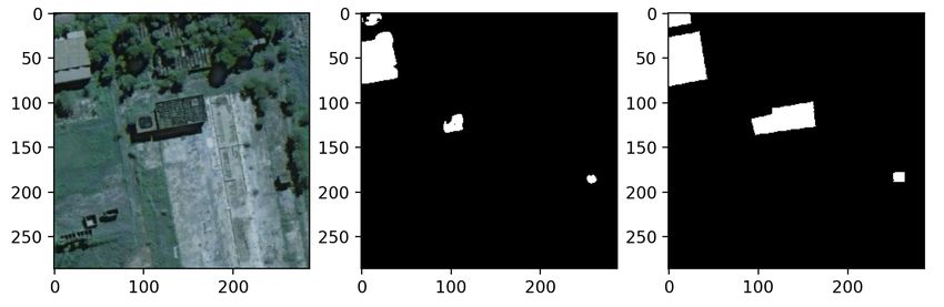
EE 5561 IMAGE PROCESSING AND APPLICATIONS, SPRING 2021                                                                                6

                                       Fig. 6: Training and Validation loss for 25 epochs.

we lose significant image resolution at each convolution step.
We observed this modification to also result in a more stable
training process. Both these modifications to the padding result
in output image sizes that are 286×286, which is conveniently
the same size as our input image. We verified that our all
tensor shapes in our network matched the original paper before
making these modifications.
   For training, we used the Adam optimizer with a learning
rate of 1 × 10⁻⁴ , weight decay of 1 × 10⁻⁸ and momentum
of 0.9. We used a batch size of 16, which saturated the
12GB of video memory we had available for training. We
also included a scheduler, which would decrease the learning
rate whenever a two-epoch plateau in the validation loss is
observed. Decreasing the learning rate in this way can result in
additional performance by avoiding overshoot of the network
weight updates during later epochs. The update gradients are
also capped at 0.1 to avoid too large of updates at each step.
   We trained the U-Net for 25 epochs with the previously
described softmax cross-entropy loss. In PyTorch, this loss
function is implemented as BCEWithLogitsLoss for bi-
nary classification. Figure 6 shows the training and validation
loss for the 25 training epochs. In each epoch we trained
the net on all the training images, then evaluated the U-Net
predictions and calculated the loss. We noted a plateau in our     Fig. 7: Top to bottom: rural, sub-urban, urban scene. Left to right:
                                                                   training images, predicted building masks, and ground truth masks.
training and validation loss after 15 epochs, so we chose these
network weights as our final model to avoid overfitting.
   Figure 7 shows training images, their predicted masks, and
                                                                   truth and predicted labels in figure 7), and found that our
ground truth masks, for two different training images. To
                                                                   network succeeded in classifying buildings at each density.
generate a final binary mask, we threshold the output of
                                                                   In dense urban environments, the network excludes roads and
our network at 0.5. All pixel values below 0.5 correspond
                                                                   courtyards, and in rural areas, false positives are low. We noted
to the label “not building” and everything greater than 0.5
                                                                   that the largest difference between our masks and the ground
correspond to the “building” label. This is unrelated to the
                                                                   truth was near building edges and when multiple buildings are
IoU thresholding performed for assessment.
                                                                   classifies as one.
                                                                      In order to calculate our U-Net results, we used the openCV
                         III. R ESULTS
                                                                   function findContours to find the boundaries of predicted
A. U-Net Segmentation Results                                      and ground truth building footprints, and calculated the IoU
  From visual inspection, we observe that the image masks          as described in section II, following the SpaceNet convention
of our U-Net segmentation network match remarkably well            of a 0.5 threshold to determine whether an IoU constitutes a
with the ground truth. We qualitatively evaluated three types      detection or not. Table I shows the true positive, true negative,
of scenes: rural, sub-urban, and urban (pictured with ground       and false negative results from our validation set. For our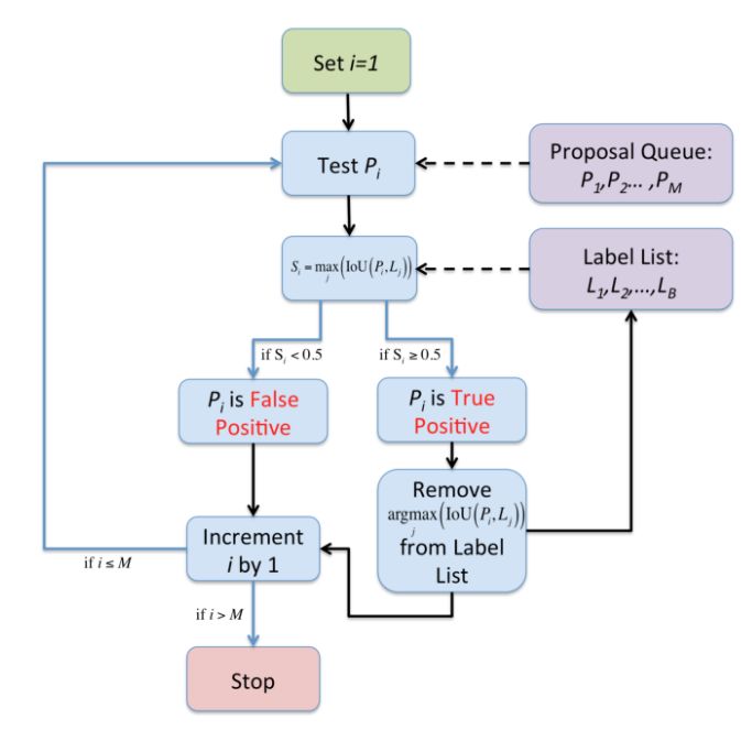
EE 5561 IMAGE PROCESSING AND APPLICATIONS, SPRING 2021                                                                                      7

problem, the concept of a true negative is not well defined: a
true negative is where there is no building in the ground truth
mask or the predicted mask, and so there is no way to “count”
the locations where we have a true negative.
   From table I it is apparent that our algorithm misses many
buildings, having a somewhat high rate of false negatives. The
number of false negatives is likely explained by the situation
                                                                                     (a) Validation image 1: building polygons
where many nearby buildings are detected as one. In this case,
only one of the buildings would be considered a true positive,
and the rest are false negatives, even though the image masks
match well. Similarly, our false positive rate could also be
skewed by the situation where a single building is detected as
two separate masks due to occlusion. We found this effect to
not be as prevalent as the many-to-one scenario. Overall our
network detected 7,333 out of 33,541 ground truth buildings.                          (b) Validation image 1: building masks
Even considering these false positive and false negative results,
our network performed similarly to the winning submissions.

        TABLE I: U-Net Building Detection Results.

                               Actual Positive        Actual Negative

        Predicted Positive          7,333                 17,192                     (c) Validation image 2: building polygons
       Predicted Negative           26,208                 N/A

   Figure 8 shows two validation images with the correspond-
ing predicted and ground truth building polygons and masks.
We see that the U-Net does a good job of finding buildings
in the image along with general shapes and orientations, but
sometimes fails to separate buildings which are close together.                       (d) Validation image 2: building masks
In addition, the U-Net predicts general shapes which tend to be         Fig. 8: Left to right: validation images, predicted building polygons
more rounded instead of having sharper corners, as the ground           & masks, and ground truth polygons & masks.
truth masks do.
   We calculated the precision, recall, and F1 as described
above from the total true positive, true negative, and false            B. SpaceNet v1 Challenge Winners
positive building detections in table I, and computed the                  To provide context on the effectiveness of our U-Net
overall F1 score from these precision and recall numbers.               building detection implementation, we present the top 3
We also calculated a simple average IoU score over all the              winning scores from the SpaceNet Building Detection v1
validation images, by taking the IoU between all predicted              Challenge. The three top scores were submitted by users
building masks and all ground truth building masks for each             wleite, Mark.cygan, and ginhaifan.
image, and averaging the result over the number of validation              The first place algorithm first put each pixel into one of
images. Note that this uses a different approach from that used         three classes: border, inside building, or outside building.
in taking the pairwise IoU to determine detections, and thus is         Then wleite used a random-forest based classificaton method
not related to the precision, recall, and F1 scores. The average        (this method did not use a deep neural network) to classify
IoU is an indication of how well our masks match the ground-            buildings, and another random forest classifier to determine
truth overall and does not consider building instance detection.        building polygon footprints. The second place algorithm from
Table II shows all four computed metrics for our validation set.        Mark.cygan used the same 3-category classification (border,
                                                                        inside building, outside building) but used a typical CNN
        TABLE II: U-Net Building Detection Results.                     classification approach. The CNN output was a heat map that
                                                                        was then converted into a polygon footprint mask. The third
          Average IoU        Precision       Recall      F1 Score       place implementation from ginhaifan used a multitask network
                                                                        cascade approach which is a deep convolution, instance aware
            0.507564         0.299001    0.218628        0.252575
                                                                        segmentation network.
                                                                           The challenge winner’s F1 scores are shown in table III,
   Note that average IoU score is significantly higher than             along with the F1 score from our U-Net implementation.
the other metrics because it is not affected by the same false             Our F1 score appears to compete with the winning imple-
negative and false positive errors described earlier.                   mentations; our score puts us between the 1st and 2nd place
EE 5561 IMAGE PROCESSING AND APPLICATIONS, SPRING 2021 8
TABLE III: SpaceNet Building Detection V1 challenge win- absence of sharp edges and corners in our predicted mask. This
ners and our U-Net results. is another result of the convolution down-sampling, and we
likely lose out on some IoU value due to the rounded corners
1st Place 2nd Place 3rd Place Our U-Net
of the predicted buildings. Some more advanced segmentation
F1 Score 0.255292 0.245420 0.227852 0.252575
networks aim to fix this by including additional skip layers
that preserve fine details in the mask.
For these reasons, the U-Net seems to be an effective
semantic segmentation method, with some limitations.
entries. However, there are several reasons why comparing our
F1 score to those reported by the winners may not be exactly
fair. V. C ONCLUSION
First, we evaluated our method on a different set of images The amount of recent activity in the development of ma-
than the winners, since we did not have access to building chine learning methods coupled with an influx of satellite
masks for the official testing image set. Second, instead of image data has motivated efforts in automatically generating
comparing geoJSON truth polygons to our building footprints, civil system maps which before recently has been impos-
we evaluated using cv2.findContours, and so some sible or very difficult. Organizations like SpaceNet play an
buildings that were close together may have been considered important role in these efforts by providing free satellite
to be single buildings (in both the ground truth images as image data sets and targeted competitions aiming to solve
well as our predictions), which could impact the IoU score common problems associated with satellite image mapping.
as well as the total number of ground truth buildings, thus Our project focused on the first SpaceNet challenge associated
increasing precision and recall. Third, our approach used an with building detection, and shows promising results.
essentially unmodified U-Net coupled with a simple contour Our solution leverages the U-net CNN architecture, a pow-
detection method to find building polygons. In many of erful method for semantic segmentation. This network deviates
the winning algorithms however, they employed complicated from the fully connected CNN in that its contraction and
multi-step approaches for both building detection and polygon expansion paths use only the valid portion of the signal from
generation. Finally, we used our own implementations of the the previous level, but makes gains in training simplicity
IoU, precision, recall, and F1 scores, which may or may not and accuracy as a result. The contraction path builds a low-
be slightly different from the official implementations. resolution feature-deep representation that maintains feature
context beyond just the desired number of output classes. The
IV. D ISCUSSION expansion path then combines this feature-deep representation
Our U-Net shows very good performance relative to the with the localized features associated with the previous con-
winners of the SpaceNet Building Detection v1 challenge, traction levels. This expansion process reduces the number
indicating that it is a powerful method for image segmentation. of features while increasing image resolution until a high-
The relative ease of implementation, and its conceptual sim- resolution image is obtained containing the desired number
plicity make it an attractive option for semantic segmentation of output segmentation classes. For our application, the U-Net
tasks. However, the method has several drawbacks. produces a segmentation mask representing either a building
First, there were some implementation quirks. Initially we or non-building.
had implemented the U-Net without padding, instead just Our results suggest that the U-Net is an effective method
cropping the input signal from one step of the contracting path for semantic segmentation, potentially competing with the
to the next. This resulted in a final segmentation mask that SpaceNet Building Detection v1 challenge winners from the
eventually became full of not-a-number (NaN) values. After original challenge. Although our U-Net misses buildings at a
adjusting the algorithm and using padding in the contracting moderately high rate, our overall IoU, precision, recall, and
and expansion paths, this was no longer an issue. F1 scores demonstrate the algorithm’s effectiveness for the
Second, our network occasionally struggles with differ- building detection segmentation task. The U-Net has several
entiating buildings when they are too close together. The limitations which could prove to be significant drawbacks
original U-Net paper attempts to improve this performance by depending on the application, but our implementation showed
including a term in the loss function that specifically weights strong results for the task of building detection.
border pixels. We believe that implementing this loss function
could improve our performance, but we leave this fine-tuning R EFERENCES
to future work.
[1] A. V. Etten, D. Lindenbaum, and T. Bacastow, “Spacenet: A remote
Finally, the U-Net sometimes shows difficulty in predicting sensing dataset and challenge series.” ArXiv, 2018.
the building sizes in the images we used. For example, in the [2] J. Jordan, “An overview of semantic image segmentation,”
bottom image of figure 7, there is a ground truth building near Online, 2018. [Online]. Available: https://www.jeremyjordan.me/
semantic-segmentation/
the middle of the image that is much larger than its predicted [3] L. Liu, W. Ouyang, X. Wang, P. Fieguth, J. Chen, X. Liu, and
counterpart. We observed that this most often happens for long, M. Pietikäine, “Deep learning for generic object detection: A survey,”
skinny buildings, which could be a byproduct of not having ArXiv, 9 2018.
[4] S. Jégou, M. Drozdzal, D. Vazquez, A. Romero, and Y. Bengio, “The
enough resolution for the convolution operations to build one hundred layers tiramisu: Fully convolutional densenets for semantic
reliable features. Another downside of our approach is the segmentation,” ArXiv, 10 2017.EE 5561 IMAGE PROCESSING AND APPLICATIONS, SPRING 2021 9
[5] M. Drozdzal, E. Vorontsov, G. Chartrand, S. Kadoury, and C. Pal,
“The importance of skip connections in biomedical image segmentation,”
ArXiv, 9 2016.
[6] P. Hagerty, “The spacenet metric,” Online, 2016. [Online]. Available:
https://medium.com/the-downlinq/the-spacenet-metric-612183cc2ddb
[7] jshermeyer, T. Stavish, dlindenbaum, N. Weir, lncohn, and W. Maddox,
“Spacenet utilities,” Online, 2017. [Online]. Available: https://github.
com/SpaceNetChallenge/utilities
[8] O. Ronneberger, P. Fischer, and T. Brox, “U-net: Convolutional networks
for biomedical image segmentation,” ArXiv, 5 2015.You can also read