Numerical simulation for bioconvectional flow of burger nanofluid with effects of activation energy and exponential heat source/sink over an ...

Page created by Esther Townsend
 
CONTINUE READING
Numerical simulation for bioconvectional flow of burger nanofluid with effects of activation energy and exponential heat source/sink over an ...
www.nature.com/scientificreports

                OPEN              Numerical simulation
                                  for bioconvectional flow of burger
                                  nanofluid with effects of activation
                                  energy and exponential heat
                                  source/sink over an inclined
                                  wall under the swimming
                                  microorganisms
                                  Hassan Waqas1, Umar Farooq1, Aqsa Ibrahim2, M. Kamran Alam3, Zahir Shah4,5* &
                                  Poom Kumam6,7*

                                  Nanofluids has broad applications such as emulsions, nuclear fuel slurries, molten plastics, extrusion
                                  of polymeric fluids, food stuffs, personal care products, shampoos, pharmaceutical industries, soaps,
                                  condensed milk, molten plastics. A nanofluid is a combination of a normal liquid component and tiny-
                                  solid particles, in which the nanomaterials are immersed in the liquid. The dispersion of solid particles
                                  into yet another host fluid will extremely increase the heat capacity of the nanoliquid, and an increase
                                  of heat efficiency can play a significant role in boosting the rate of heat transfer of the host liquid. The
                                  current article discloses the impact of Arrhenius activation energy in the bioconvective flow of Burger
                                  nanofluid by an inclined wall. The heat transfer mechanism of Burger nanofluid is analyzed through
                                  the nonlinear thermal radiation effect. The Brownian dispersion and thermophoresis diffusions effects
                                  are also scrutinized. A system of partial differential equations are converted into ordinary differential
                                  equation ODEs by using similarity transformation. The multi order ordinary differential equations
                                  are reduced to first order differential equations by applying well known shooting algorithm then
                                  numerical results of ordinary equations are computed with the help of bvp4c built-in function Matlab.
                                  Trends with significant parameters via the flow of fluid, thermal, and solutal fields of species and
                                  the area of microorganisms are controlled. The numerical results for the current analysis are seen in
                                  the tables. The temperature distribution increases by rising the temperature ratio parameter while
                                  diminishes for a higher magnitude of Prandtl number. Furthermore temperature-dependent heat
                                  source parameter increases the temperature of fluid. Concentration of nanoparticles is an decreasing
                                  function of Lewis number. The microorganisms profile decay by an augmentation in the approximation
                                  of both parameter Peclet number and bioconvection Lewis number.

                                  1
                                   Department of Mathematics, Government College University Faisalabad, Layyah Campus, Faisalabad 31200,
                                  Pakistan. 2Department of Physics, Government College University Faisalabad, Faisalabad 38000,
                                  Pakistan. 3Department of Pure & Applied Mathematics, The University of Haripur, Khyber Pakhtunkhwa 22620,
                                  Pakistan. 4Department of Mathematical Sciences, University of Lakki Marwat, Lakki Marwat 28420, Khyber
                                  Pakhtunkhwa, Pakistan. 5Center of Excellence in Theoretical and Computational Science (TaCS‑CoE), Faculty
                                  of Science, Thonburi (KMUTT), King Mongkut’s University of Technology, 126 Pracha Uthit Rd., Bang Mod,
                                  Thung Khru, Bangkok 10140, Thailand. 6Fixed Point Research Laboratory, Fixed Point Theory and Applications
                                  Research Group, Center of Excellence in Theoretical and Computational Science (TaCS‑CoE), Faculty of Science,
                                  King Mongkut’s University of Technology Thonburi (KMUTT), 126 Pracha Uthit Rd., Bang Mod, Thung Khru,
                                  Bangkok 10140, Thailand. 7Department of Medical Research, China Medical University Hospital, China Medical
                                  University, Taichung 40402, Taiwan. *email: zahir@ulm.edu.pk; poom.kum@kmutt.ac.th

Scientific Reports |   (2021) 11:14305               | https://doi.org/10.1038/s41598-021-93748-x                                            1

                                                                                                                                         Vol.:(0123456789)
www.nature.com/scientificreports/

                                             Abbreviations
                                             (u&v)	Velocity components, ­ms−1
                                             (αm )	Thermal diffusivity
                                             (α)	Inclination of the wall
                                            γ 	            Microorganisms average volume, m ­ 3
                                              ρf 	Density of fluid, ­kgm−3
                                                 

                                            Wc	            Cell Swimming Speed, ­ms−1
                                              ρcp p	Heat Capacitance of nanoparticles, J­ m−3 ­K−1
                                                    

                                              ρcp f 	Heat Capacitance of fluid, J­ m−3 ­K−1
                                             

                                            ρm∗	           Density of Motile Microorganisms, ­kgm−3
                                              g 	Acceleration due to gravity
                                                 
                                             (σ )	Electrical conductivity
                                             σ1	Chemical reaction parameter
                                             β ∗∗	Thermal suspension coefficient, K        ­ −1
                                             (T)	Temperature K
                                             (�)	Concentration of nanoparticles, m         ­ olL−1
                                             (N)	Motile microorganisms, ­m−3
                                             (DB )	Brownian motion coefficient, m       ­ 2s−1
                                             (DT )	Thermophoresis diffusion coefficient, m         ­ 2s−1
                                                                                          2 −1
                                             Dm	Microorganisms coefficient, ­m s
                                             (1 &2 )	Relaxation effects
                                             (3 )	Retardation effect
                                             (β1 , β2 &β3 )	Deborah numbers
                                            (Nr)  	Buoyancy ratio parameter
                                              M 2 	Hartman number
                                             (S)	Mixed convection parameter
                                             Kr 2	Chemical reaction constant, s­ −1
                                             (Nc)	Bioconvection Rayleigh number
                                             hf 	Convective heat transfer coefficient, W         ­ m2K−1
                                             hg 	Concentration transfer coefficient, m         ­ s−1
                                             hn	Microorganisms transfer coefficient, m            ­ s−1
                                             (Nb)	Brownian motion parameter
                                             (Pr)	Prandtl number
                                             (Rd)	Radiation parameter
                                            (θw∗)	Temperature ratio parameter
                                            QT∗ 	Thermal dependent heat source coefficient
                                              QE 	Exponential space dependent heat source
                                             (QE )	Exponential space bases source parameter
                                             (QT )	Temperature dependent Heat source parameter
                                             (QE )	Exponential space bases source parameter
                                             (Nt)	Thermophoresis parameter
                                             (Le)	Lewis’s number
                                             (Lb)	Bioconvection Lewis number
                                             (δ1 )	Microorganism difference parameter
                                             (Pe)	Peclet number
                                             (C)	Marangoni number
                                             (D)	Marangoni ratio parameter
                                             (S1 )	Thermal Biot number
                                             (S2 )	Concentration Biot number
                                             (S3 )	Microorganism Biot number
                                             σq	Boltzmann constant
                                             k∗	Means absorption coefficient
                                             σT 	Temperature surface tension coefficient
                                             σ�	Coefficient of concentration surface tension
                                             qs	Heat flux
                                             qn	Motile density flux
                                             qw	Mass flux
                                             (Nu)	Nusselt number
                                             (Sh)	Sherwood number
                                             (Sn)	Microorganism’s density number

                                            Due to the significant applications in the engineering field, nanofluids have drawn the interest of many scien-
                                            tists. The heat transition of convection liquids such as ethylene glycol, kerosene, water and oil can be used in a
                                            wide variety of engineering tools, such as electron and heat transfer instruments. Nanofluids are the combina-
                                            tion of smaller nanomaterials and a base fluid. As a consequence, the presence of micro solid objects in typical
                                            fluids has enhanced the characteristics of heat transformation. There are many potentials uses of nanofluids for
                                            heat transfer, namely cooling systems, air conditioners, chillers, microelectronics, computer microchips, diesel
                                            engine oil and fuel cells. It should be remembered that the thermal conductivity of nanomaterials is improved

          Scientific Reports |   (2021) 11:14305 |               https://doi.org/10.1038/s41598-021-93748-x                                                 2

Vol:.(1234567890)
www.nature.com/scientificreports/

                                  by volume fraction, particulate size, pressure, including thermal conductivity. Nanotechnology is of consider-
                                  able interest in a variety of industries, including chemical and metallurgical equipment, shipping, macroscopic
                                  artifacts, medical treatments, and electricity generation. Nanofluids are mixtures of nanometer-sized particulate
                                  suspensions with conventional fluids, including one that was presented by ­Choi1. ­Buongiorno2 explores the two
                                  peculiar sliding mechanisms, in particular, the Brownian diffusion and thermophoresis influence, to enhance the
                                  normal convection rate of the heat energy distribution. Venkatadri et al.3 researched a melting heat transport of
                                  an electrical nanofluid flow conductor towards an exponentially shrank/extended porous layer with nonlinear
                                  radiative Cattaneo-Christov heat flux under a magnetic field. Mondal et al.4 have studied the impact of the heat
                                  exchange of magnetohydrodynamics on the stagnation point flow over the extended or decreasing surface by
                                  homogeneous chemical reactions. Ying et al.5 examined radiative heat transmission of molten salt-based flow
                                  of nanofluid over a non-uniform heat flux. Zainal et al.6 tracked the MHD hybrid nanofluid flow to the porous
                                  expansion/reduction sheet at the presence of a quadratic momentum. Eid et al.7 identified a shift in thermal
                                  conductivity, namely heat transfer effects on the magneto-water nanofluid flow in a porous slippery channel.
                                  Numerous researchers are involved in the Burger nanofluid seen in R      ­ ef8–23.
                                      The process of bioconvection can be described as the swimming up of microbes in materials, which are less
                                  dense than water. owing to the advanced concentration of microorganisms, above that the layer of substances
                                  happens to too thick and delicate, which allows the microorganisms to break down owing to the bioconvec-
                                  tion flow. Microorganisms, many of which are older organisms on the globe known as human beings, are very
                                  important in many ways. It is defined as a type of growth of microorganism substances, such as bacteria or
                                  algae, due to the up-swimming microorganism. Bioconvection has many uses in the world of biochemistry
                                  and bioinformatics. The Bioconvection process is used by bioengineering in diesel fuel goods, bioreactors, and
                                  fuel cell engineering. P­ latt24 was the very first person to describe bioconvection phenomena. Unstable density
                                  distributions were adopted as a technique for the arrangement of suspensions of swim motile microorganisms
                                  and the term bioconvection was created. K     ­ uznetsov25 subsequently introduced this idea based on nanofluids,
                                  namely gyrotactic motile microorganisms, suggesting that the resultant large-scale flow of fluid produced by
                                  self-propelled motile gyrotactic microorganisms increases the mixture and prevents nanomaterials aggregation
                                  in nanofluids. Haq et al.26 studied the flow properties of Cross Nanoparticles across expanded surfaces subject to
                                  Arrhenius activation energy and magnetization field. Ahmad et al.27 examined a bioconvection nanofluid flow
                                  comprising gyrotactic motile microorganisms with a chemical reaction allowance through a porous medium
                                  past a stretched surface. Elanchezhian et al.28 worked on the rate of motile gyrotactic microorganisms in the
                                  bioconvective nanofluid flow of Oldroyd-B past a stretching sheet with a mixing convective and inclination
                                  magnetization area. Bhatti et al.29 performed a mathematical analysis on the migration of motile swimming
                                  microorganisms in non-Newtonian blood-based nanoliquid by anisotropic artery restriction. Khan et al.30 illus-
                                  trated the essential rheological characteristics of Jeffrey’s gyrotactic motile microorganism–like nanofluid by
                                  rapid development. Shafiq et al.31 assessed the rate of heat and mass transition of gyrotactic microorganisms
                                  with the second-grade nanofluid flow. Kotnurkar et al.32 addressed the bioconvection of 3rd-grade nanoliquid
                                  flowing by copper-blood nanofluids in porous walls, consisting of motile species. Muhammad et al.33 recognized
                                  the time-dependent motion of thermophysical magnetization Carreau nanofluids, which convey motile micro-
                                  organisms via a spinning wedge through velocity slip as well as thermal radiation features. Farooq et al.34 have
                                  introduced an entropic example of the 3-D bioconvective movement of nanoliquid across a linearly spinning
                                  plate in the absence of magnetic influences. Hosseinzadeh et al.35 investigated the flow of motile microorganisms
                                  and nanotechnology through a 3-D stretching cylinder. Any important and most recent work of bioconvection
                                  swimming fluid microorganisms has been analyzed analytically by a variety of fascinating ­investigators36–40.
                                      Our inspiration of the present study is to examine the model of the Burger nanofluid with activation energy
                                  and exponential heat source/sink through inclined wall. The behaviors of Brownian motion and thermophoresis
                                  diffusion effects are scrutinized. Bioconvection and motile microorganisms is also discussed. The novelty of this
                                  work is investigating the 2D flow of Burger nanoliquid past an inclined wall. The dimensionless ODEs are tackled
                                  with shooting method to reduce the order via bvp4c MATLAB tool. The careful study of literature shows that the
                                  mathematical formulation established in this communication is novel and has not been talked before as per the
                                  author’s data. The physical performance of parameters via flow profiles are survey via graphical and tabular data.

                                  Mathematical formulation
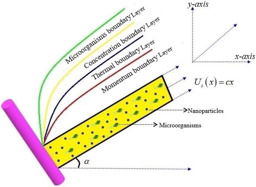
                                  This model appraises the two-dimensional Bioconvectional flow of Burgers nanofluid containing swimming
                                  gyrotactic microorganisms over a vertical inclined wall. The Brownian motion and thermophoresis diffusion are
                                  considered for nanofluid. Heat and mass transfer aspects are found to be associated with the exponential space
                                  based heat source. The velocity of the wall is Us (x) = cx and the magnetic field is along the transverse direction.
                                  The inclined wall is clarified in Fig. 1. Basic laws describing the conservation of mass and momentum yield.
                                                                                         divV = 0,                                                (1)

                                                                                    DV
                                                                                ρ      = −∇p + divS,                                              (2)
                                                                                    Dt

                                      The extra stress tensor of burger fluid model is
                                                                                     D2 S
                                                                                                       
                                                                              DS                    DA1
                                                                     S + 1      + 2 2 = µ A1 + 3       .                                       (3)
                                                                              Dt     Dt              Dt

Scientific Reports |   (2021) 11:14305 |               https://doi.org/10.1038/s41598-021-93748-x                                                   3

                                                                                                                                               Vol.:(0123456789)
www.nature.com/scientificreports/

                                            Figure 1.  Flow pattern of the problem.

                                                The modeled boundary layer equations for the nanofluid flow model are represented as f­ ollows41: In the expi-
                                            rations (3 ) is the retardation effect and (1 &2 ) are relaxation effects. It is marked out here that the outcomes
                                            for the Oldroyd-B fluid model can be deduced for (2 = 0) and the findings for the Maxwell fluid model can be
                                            reduced (2 = 3 = 0). Also, the effects of the Fluid model can be extracted by specifying (1 = 2 = 3 = 0).
                                                                                                        3
                                                                                                         u uxxx + v 3 uyyy + u2 uxx ux − uy vxx + 2vx uxy
                                                                                                                                   �                       �

                                                  uux + vuy + 2 u2 uxx + v 2 uyy + 2uvuxy + 3  3v 2 vy uyy + uy uxy + 3uv uuxxy + vuxyy
                                                                    �                         �             �                 �       �               �    
                                                                                                                                                            
                                                                                                             �                                   �
                                                                                                         2uv uy uxx + vx uyy + vy uxy − uy vxy
                                                                                                                �                    �                  ��
                                                      �           �                                  �� σ B02                          uvx uy − vux uy         (4)
                                                  = ν uyy + 3 uuxyy + vuyyy − ux uyy − uy vyy −                  u + 1 vuy + 2
                                                                                                            ρf                         +uvuxy + v 2 uyy
                                                               ��                                                             �
                                                                  1 − �f ρf β ∗∗ g ∗ (T − T∞ ) − ρp − ρf g ∗ (� − �∞ )
                                                                          �                         �        �
                                                             1
                                                  + cos α                                                                        ,
                                                            ρf −(N − N∞ )g ∗ γ ρm − ρf
                                                                                  �         �

                                                                                                                    3
                                                                                                                         
                                                                                                   DT  2      16σq T∞
                                                                 uTx + vTy = αm Tyy + τ DB �y Ty +     Ty   +        Tyy
                                                                                                   T∞          3k∗ ρcp f
                                                                                                                                                              (5)
                                                                    QT∗                 QE∗                 c 0.5
                                                                 +   (T − T∞ ) +   (T − T∞ ) exp −            ny ,
                                                                    ρcp f              ρcp f                vf

                                                                                                                      T m
                                                                                                                                  
                                                                                            DT                                  −Ea
                                                                u�x + v�y = DB �yy +           Tyy − Kr 2 (� − �∞ )       exp         ,                           (6)
                                                                                            T∞                       T∞         K1 T

                                                                                                             bWc
                                                                                                                                                                  (7)
                                                                                                                        
                                                                            uNx + vNy = Dm Nyy −                      ∂y N�y ,
                                                                                                          (�s − �∞ )
                                                With relative boundary ­conditions42:
                                                                                   �          �                          
                                                                     u = Us , µuy �       σ         = σT Tx |y=0 −σ� �x |y=0 ,
                                                                                              �
                                                                                       y=0 x �y=0
                                                                                                                        
                                                                                                                        
                                                                                                                        
                                                                                                                        
                                                                                                                        
                                                                                                                        
                                                                        −kTy = hf (Ts − T), −DB �y = hg (�s − �),         ,                                       (8)
                                                                        −Dm Ny = hn (Ns − N), at y = 0,
                                                                                                                        
                                                                                                                        
                                                                                                                        
                                                                                                                        
                                                                                                                        
                                                                        u = 0, v = 0, T → T∞ , � → �∞ , N → N∞ as y → ∞.
                                                                                                                        

                                             Here in the
                                                       above equation
                                                                       (u&v) are velocity components, (αm ) is thermal diffusivity, (α) is the inclination of
                                             the wall, ρf is density, g ∗ acceleration due to gravity, (σ ) is electric conductivity, (T) is temperature, σq signifies
                                            Boltzmann    constant, k∗ denotes means absorption coefficient, (DB ) is Brownian motion coefficient,
                                                       
                                              τ = ρcp p ρcp f is ratio of nanoparticle heat capability to heat capability of fluid, σT be the temperature
                                             surface tension coefficient, σ� is the coefficient of concentration surface tension and (DT ) is thermophoresis
                                             coefficient.
                                                Following suitable similarity transformations are used for normalizing the system of PDE 41:

          Scientific Reports |   (2021) 11:14305 |                https://doi.org/10.1038/s41598-021-93748-x                                                        4

Vol:.(1234567890)
www.nature.com/scientificreports/

                                                                       �
                                                                                                   √
                                                                                                                            
                                                                         c
                                                                 ζ =       y, u = cxf ′ (ζ ), v = − cνf (ζ ),               
                                                                                                                            
                                                                         ν
                                                                                                                            
                                                                                                                             ,                                       (9)
                                                                          T − T∞                 � − �∞            N − N∞ 
                                                                 θ(ζ ) =           , φ(ζ ) =             , χ(ζ ) =         .
                                                                                                                            
                                                                          Ts − T∞               �s − � ∞           Ns − N∞
                                      The reduced system will:

                                                         f ′′′ − f ′2 + ff ′′ + β1 2ff ′ f ′′ − f 2 f ′′′ + β2 f 3 f iv − 2ff ′2 f ′′ − 3f 2 f ′′2
                                                                                                                                                
                                                                                                                                                                     (10)
                                                         +β3 f ′′2 − ff iv − M 2 f ′ − β1 ff ′′ + β2 f 2 f ′′′ + cos αS(θ − Nrφ − Ncχ) = 0,
                                                                                                               

                                  Here                    ), β2 =c 2 2 &β3 (= c3 ) are Deborah numbers, the buoyancy ratio parameter
                                                                           
                                       β1 (= c     1
                                              ρp −ρf (�s −�∞ )
                                                                                     2
                                                                             2 = σ B0 is the Hartman number, the mixed convection parameter is
                                  Nr = (1−�                       ∗∗ , M           ρf c
                                                    ∞ )(T∞ )ρf β
                                                                                                                                                      
                                         β ∗∗ g ∗ (1−�∞ )(Ts −T∞ )
                                                                     
                                                                                                                                    γ ρm −ρf (Ns −N∞ )
                                  S =                aUs                , the bioconvection      Rayleigh   number     is Nc   =     (1−�∞ )(T∞ )ρf β ∗∗ .

                                              1 + Rd 1 + (θw − 1)θ 3 θ ′′ + Pr f θ ′ − 2f ′ θ + Nbφ ′ θ ′ + Ntθ ′2 + QT θ + QE exp (−nζ ) = 0, (11)
                                                                                                                              

                                                                                                                                                               16σ ∗ T 3
                                                                                                                                                                    
                                  Here Nb = τ DB (�αsm−�∞ ) is the Brownian motion parameter, Pr = ανm is the Prandtl number, Rd = 3kk∗∞
                                                                                                                                                 
                                                                                                                                          Q∗
                                                                                    
                                  is the radiation parameter, θw = TT∞s is temperature ratio parameter, QT = (ρc T) a is temperature dependent
                                                                                                                                         p f
                                                                                         Q∗
                                  heat source/sink parameter, QE = (ρc E) a be the exponential space-based heat source/sink parameter,
                                                                                        p f
                                           τ DT (Ts −T∞ )
                                  Nt =           T∞ αm          is the thermophoresis parameter.
                                                                                                                                                   
                                                                                           Nt ′′                                          −E
                                                           φ ′′ + Le Pr f φ ′ − 2f ′ φ +           θ − Le Pr σ1 (1 + δθ)m exp                                        (12)
                                                                           
                                                                                                                                                      φ = 0,
                                                                                                Nb                                       1 + δθ
                                                                                            2
                                  Here Le = αDmB is Lewis’s number, σ1 = Krc be the chemical reaction parameter, E = K1ETa∞ signifies the activa-
                                  tion energy, δ = TsT−T       ∞
                                                                  ∞
                                                                     clarify the temperature difference parameter.
                                                                                χ ′′ + Lbf χ ′ − Pe φ ′′ (χ + δ1 ) + χ ′ φ ′ = 0,                                    (13)
                                                                                                                              
                                                                                                                       
                                  Here
                                     
                                         Lb = Dνm is bioconvection Lewis number, δ1 = NsN−N
                                                  
                                                                                                                     ∞
                                                                                                                        ∞
                                                                                                                            is microorganism difference parameter
                                        Dm is Peclet number.
                                  Pe = bW c

                                     With dimensionless boundary constraints:
                                                                 f (ζ ) = 0, f ′ (ζ ) = −C(1 + D),
                                                                                                                                      
                                                                                                                                      
                                                                                                                                      
                                                                 θ ′ (ζ ) = −S1 (1 − θ(ζ )), φ ′ (ζ ) = −S2 (1 − φ(ζ )),
                                                                                                                                      
                                                                                                                                      
                                                                                                                                         ,                          (14)
                                                                 χ ′ (ζ ) = −S3 (1 − χ(ζ )), atζ = 0,                                 
                                                                                                                                      
                                                                                                                                      
                                                            f ′ (ζ ) → 0, θ(ζ ) → 0, φ(ζ ) → 0, χ(ζ ) → 0, as ζ → ∞.
                                                                                                                                      
                                                                                                                                                
                                                                                                                                              hf  ν
                                  Here C = µc          is
                                                σT A  ν
                                                    a     the
                                                             Marangoni       number,  and D   = σ� B
                                                                                                  σT A   is Marangoni ratio parameter, S1   = k    a is
                                                                                                                            
                                                                   hg  ν
                                  thermal Biot number, S2 = DB a is concentration Biot number, S3 = Dm a is microorganism Biot
                                                                                                                       hn  ν

                                  number.
                                     The shear stress of Burger fluid describes a­ s10
                                                                       D2
                                                                                                
                                                            D                            ∂u     ∂v
                                                    1 + 1        + 2         Sxy = µ      +
                                                            Dt         Dt 2              ∂y     ∂x
                                                         
                                                                 2          2                  2                  2  2                        (15)
                                                              ∂ u        ∂ u        ∂v       ∂ v         ∂u ∂v      ∂u         ∂v
                                                  +µ3 u             +v 2 +u 2 +v                  −2          −          −
                                                             ∂x∂y        ∂y         ∂x      ∂x∂y         ∂y ∂x      ∂y         ∂x

                                  Here above equation signifies that it is impossible to write shear stress in current case in terms of component of
                                  velocity u, v . It shows the way to detail that shear stress according in terms of f and derivative with respect to ζ
                                  by using transformation (9). According to this point of view, one cannot calculate skin friction in this situation
                                  because
                                                                                                 
                                                                                             Sxy y=0
                                                                                      Cf =            .                                           (16)
                                                                                               ρUw2
                                      In which skin friction for viscous fluid (1 , 2 , 3 = 0) is f ′′ (0).
                                      The Nusselt number, Sherwood number, and microorganism’s density number can be described as:

Scientific Reports |   (2021) 11:14305 |                   https://doi.org/10.1038/s41598-021-93748-x                                                                   5

                                                                                                                                                                 Vol.:(0123456789)
www.nature.com/scientificreports/

                                                                                 xqs                 xqw                  xqn
                                                                     Nu =
                                                                             k(Ts − T∞ )
                                                                                         , Sh =
                                                                                                DB (�s − �∞ )
                                                                                                              , Sn =
                                                                                                                     Dm (Ns − N∞ )
                                                                                                                                   ,                           (17)

                                                                                                                 
                                                                         qs = −k Ty y=0 , qw = −DB y y=0 , qn = −Dm Ny y=0 ,                                  (18)

                                                Hence, the dimensionless form of engineering quantities is given by
                                                                              Nu                   Sh                   Sn
                                                                                1   = −θ ′ (ζ ),     1   = −φ ′ (ζ ),      1   = −χ ′ (ζ ),                    (19)
                                                                                2                    2
                                                                              Rex                  Rex                  Rex2

                                            Numerical approach
                                            The two-dimensional nanofluid movement of Burgers fluid over the inclined wall is discussed in this sec-
                                            tion. Momentum, temperature, the concentration of nanomaterials, and swimming motile microorganism
                                            Eqs. (10–14) with relevant convective boundary conditions (14) are converted to a stronger non-dimensional
                                            system of ordinary differential equations using similarity transformations. Various values of several parameters
                                            are resolved numerically using the MATLAB computational toot inherent in bvp4c. This bvp4c process is used
                                            for three Lobatto-IIIa formulas. This formula is used for collective numerical results. Introduce the following
                                            new variables expressed as:
                                                Let,

                                                                             f = p1 , f ′ = p2 , f ′′ = p3 , f ′′′ = p4 , f iv = p4′ ,
                                                                                                                                      
                                                                                                                                      
                                                                                                                                      
                                                                             θ = p5 , θ ′ = p6 , θ ′′ = p6′ ,
                                                                                                                                      
                                                                                                                                      
                                                                                         ′           ′′    ′
                                                                                                                                        ,               (20)
                                                                             φ = p7 , φ = p8 , φ = p8 ,                               
                                                                                                                                      
                                                                                                                                      
                                                                                                                                      
                                                                             χ = p9 , χ ′ = p10 , χ ′′ = p10  ′
                                                                                                                  ,
                                                                                                                                      

                                                                  −p4 + p22 − p1 p3 − β1 2p1 p2 p3 − p12 p4 − β2 −2p1 p22 p3 − 3p12 p32
                                                                                                                                     

                                                                  −β3 p32 + M 2 p2 − β1 p1 p3 + β2 p12 p4 − cos αS p5 − Nrp7 − Ncp9                            (21)
                                                                                                                                     
                                                              ′
                                                             p4 =                             3                                           ,
                                                                                              β2 p1 − β3 p1

                                                                         − Pr p1 p6 − 2p2 p5 + Nbp8 p6 + Ntp62 − QT p5 − QE exp (−nζ )
                                                                                                             
                                                                 p6′ =                                                                 ,                       (22)
                                                                                             1 + Rd 1 + (θw − 1)p53


                                                                                         Nt ′                                  −E
                                                             p8′ = −Le Pr p1 p8 − 2p2 p7 −    p6 + Le Pr σ1 (1 + δp5 )m exp                                    (23)
                                                                         
                                                                                                                                       p7 ,
                                                                                           Nb                                 1 + δp5

                                                                                ′
                                                                                   = −Lbp1 p10 + Pe p8′ p9 + δ1 + p10 p8 ,                                     (23)
                                                                                                                     
                                                                               p10

                                                With
                                                                                          �                                                   
                                                                      p1 (ζ ) = 0, p2 (ζ )� = −C(1 + D),                                      
                                                                                                                                              
                                                                                    �           �              �           �                  
                                                                                                                                              
                                                                      p6 (ζ ) = −S1 1 − p5 (ζ ) , p8 (ζ ) = −S2 1 − p7 (ζ ) ,                 
                                                                                      �          �                                             ,               (24)
                                                                      p10 (ζ ) = −S3 1 − p9 (ζ ) , atζ = 0,                        
                                                                                                                                   
                                                                                                                                   
                                                                                                                                   
                                                                      p2 (ζ ) → 0, p5 (ζ ) → 0, p7 (ζ ) → 0, p9 (ζ ) → 0, as ζ → ∞.
                                                                                                                                   

                                            Results and discussion
                                            In this section, the physical behavior of various parameters (buoyancy ratio parameter, Hartman number, mixed
                                            convection parameter, thermophoresis parameter, Brownian motion parameter, Prandtl number, temperature
                                            ratio parameter, thermal dependent heat source/sink parameter, exponential space dependent heat source/
                                            sink parameter, Lewis’s number, bioconvection Lewis number, bioconvection Rayleigh number, Peclet number,
                                            Marangoni number, Marangoni ratio parameter, thermal Biot number, concentration Biot number, and micro-
                                            organism Biot number ) against subjective flow fields are discussed in detail and depicted through Fig. 2, 3, 4,
                                            5, 6, 7, 8, 9, 10, 11, 12, 13 and 14. Figure 2 is designed to notice the trends of velocity field f ′ with exaggerate of
                                            distinguishing Marangoni number C and Marangoni ratio parameter D. It is analyzed that the higher values of the
                                            Marangoni number C and Marangoni ratio parameter D provide a enhancing trend in the velocity of the fluid f ′.
                                            Figure 3 reveals the behavior of the Hartman number M and β2 on the flow of rate type nanomaterials f ′ . Veloc-
                                            ity f ′ curves preserve reducing phenomenon for greater Hartman number M and β2. Variation of velocity field
                                             f ′ with mixed convection parameter S and β3 is captured in Fig. 4. It is seen that velocity of rate type nanoliquid
                                            rises for larger magnitudes of S also depicted that velocity is increased for higher estimation of β3. The physical
                                            explanation referred to like enhancing trend is justified as mixed convection parameter currents the ratio between
                                            buoyancy force to viscous force. The outcomes of temperature distribution θ against temperature ratio parameter

          Scientific Reports |   (2021) 11:14305 |                https://doi.org/10.1038/s41598-021-93748-x                                                      6

Vol:.(1234567890)
www.nature.com/scientificreports/

                                  Figure 2.  Significance of C&D for f ′.

                                  Figure 3.  Significance of M&β2 for f ′.

                                  Figure 4.  Significance of β3 &S for f ′.

                                  θw and Prandtl number Pr are validated in Fig. 5. The temperature distribution θ rises by the uprising temperature
                                  ratio parameter θw while dwindles for a higher amount of Prandtl number Pr . The estimation in temperature
                                  distribution θ concerning thermal Biot number S1 and exponential space dependent source/sink parameter QE
                                  is displayed in Fig. 6. From the curves of thermal Biot number S1 and exponential space dependent source/sink
                                  parameter QE , it is observed that enhance in thermal Biot number S1 and exponential space dependent source/

Scientific Reports |   (2021) 11:14305 |                https://doi.org/10.1038/s41598-021-93748-x                                                7

                                                                                                                                             Vol.:(0123456789)
www.nature.com/scientificreports/

                                            Figure 5.  Significance of Pr&θw for θ.

                                            Figure 6.  Significance of QE &S1 for θ.

                                            Figure 7.  Significance of QT &Nt for θ.

                                            sink parameter QE enhances temperature distribution θ . Figure 7 examined features of the thermophoresis
                                            parameter Nt and thermal dependent source/sink parameter QT for temperature distribution θ . One can depict
                                            from this figure thermal field θ is increase with a higher amount of both the physical parameter thermophoresis
                                            parameter Nt and thermal dependent source/sink parameter QT .From physical point of view, we can say that an
                                            upsurge in the strength of thermophoresis affects an effective movement of the nanomaterials which improves the

          Scientific Reports |   (2021) 11:14305 |               https://doi.org/10.1038/s41598-021-93748-x                                              8

Vol:.(1234567890)
www.nature.com/scientificreports/

                                  Figure 8.  Significance of C&D for θ.

                                  Figure 9.  Significance of C&D for φ.

                                  Figure 10.  Significance of E&S2 for φ.

                                  thermal conductivity of the fluid which outcomes into augmentation of the fluid temperature. Figure 8 is captured
                                  to illustrate the behavior of the Marangoni number C and Marangoni ratio parameter D against a thermal field
                                  of species θ . It is scrutinized that the thermal field of species θ is declined for higher estimation of Marangoni
                                  number C and Marangoni ratio parameter D . The impression of the Marangoni number C and Marangoni ratio
                                  parameter D on the volumetric concentration of nanoparticles φ is demonstrated in Fig. 9. The reduction in

Scientific Reports |   (2021) 11:14305 |               https://doi.org/10.1038/s41598-021-93748-x                                                  9

                                                                                                                                              Vol.:(0123456789)
www.nature.com/scientificreports/

                                            Figure 11.  Significance of Nb&Nt for φ.

                                            Figure 12.  Significance of Pr &Le for φ.

                                            Figure 13.  Significance of C&D for χ.

                                            the concentration field φ is scrutinized by growing the magnitude of the Marangoni number C and Marangoni
                                            ratio parameter D . Figure 10 illustrates the impact of activation energy parameter E and concentration Biot
                                            number S2 on the concentration of nanoparticles φ . It is analyzed that the concentration ofspecies φ boosted up
                                            with larger activation energy parameter E and concentration Biot number S2.Fig. 11 is captured to scrutinize
                                            the behavior Nt and Brownian motion parameter Nb against the rescaled density of the concentration profile

          Scientific Reports |   (2021) 11:14305 |               https://doi.org/10.1038/s41598-021-93748-x                                              10

Vol:.(1234567890)
www.nature.com/scientificreports/

                                  Figure 14.  Significance of Lb & Pe for χ.

                                   Flow parameters                         Local skin friction coefficients
                                          M     Nr    Nc      C     D     −f ′′ (0)
                                   0.1                                     1.0172
                                   0.6     0.1   0.5   0.5     0.4   0.4   1.0167
                                   1.2                                     1.0057
                                           0.2                             1.0255
                                   0.2     0.5   0.5   0.5     0.4   0.4   1.0942
                                           0.7                             1.1880
                                                 0.2                       1.0066
                                   0.2     0.1   1.0   0.5     0.4   0.4   1.0275
                                                 2.0                       1.0292
                                                       0.2                 1.9265
                                   0.2     0.1   0.5   1.0     0.4   0.4   1.0281
                                                       2.0                 1.3283
                                                               0.5         1.3532
                                   0.2     0.1   0.5   0.5     0.8   0.4   1.4843
                                                               1.1         3.6851
                                                                     0.5   1.1039
                                   0.2     0.1   0.5   0.5     0.4   1.0   1.6118
                                                                     1.5   2.1507

                                  Table 1.  Outcomes of −f ′′ (0) versus flow parameter.

                                  φ . The concentration profile φ upsurges for thermophoresis parameter Nt while reducing for Brownian motion
                                  parameter Nb. Physically when we increase the thermophoresis and Brownian motion, the thermal efficiency of
                                  fluid rises. From this scenario noticed that the thermophoresis is also increased which tends to move nanopar-
                                  ticles from warm to cold sections. Features of concentration profile φ over the Prandtl number Pr and Lewis’s
                                  number Le for concentration are plotted in Fig. 12. From the curves of the concentration profile declines for the
                                  Larger Prandtl number Pr. Physically, Prandtl number illustrates ratio between momentum diffusivity to thermal
                                  diffusivity. Furthermore, Lewis’s number Le causes a reduction in the volumetric concentration nanoparticle
                                  field φ . Figure 13 is prepared to estimate the trends of Marangoni number C and Marangoni ratio parameter D
                                  against the concentration of microorganism χ . Here the concentration of microorganism χ depressed with a
                                  larger estimation of Marangoni number C and Marangoni ratio parameter D. The salient characteristics of Peclet
                                  number Pe and Lb against microorganism concentration χ are examined through Fig. 14. The microorganism’s
                                  profile χ decline by an increment in the estimation of both parameter Peclet number Pe and bioconvection Lewis
                                  number Lb. Physically the microorganism’s density of motile microorganisms always is reduced due to a higher
                                  estimation of the Peclet number.
                                       In this slice, the numerical outcomes of versus parameters via −f ′′ (0),−θ ′ (0),−φ ′ (0) and −χ ′ (0) are examined
                                  in Tables 1, 2, 3 and 4. Table 1 is calculated to investigate the trend of local skin friction coefficient −f ′′ (0) via
                                  flow parameters. The local skin friction coefficient −f ′′ (0) increased via C and D while decline for . Table 2 is
                                  explored to scrutinize the aspects of local Nusselt number −θ ′ (0) for flow parameters. From mathematical data
                                  investigation, it is examined that local Nusselt number −θ ′ (0) reduces with the improvement of Nb . Table 3
                                  reveals the variation of local Sherwood number φ ′ (0) via greater estimations of different parameters. From this
                                  table disclosed that local Sherwood number −φ ′ (0) rises for Pr&S2. The numerical outcomes of local microorgan-
                                  ism numbers −χ ′ (0) via flow parameters are shown in Table 4. Now local density number of −χ ′ (0) enhanced
                                  for higher variations C&Lb . Table 5 presents a comparative work of the current outcomes with refs. 8,43. Here
                                  good agreement is observed with current results and published literature Ref. 8,43.

Scientific Reports |   (2021) 11:14305 |                     https://doi.org/10.1038/s41598-021-93748-x                                                 11

                                                                                                                                                    Vol.:(0123456789)
www.nature.com/scientificreports/

                                             Flow parameters                                        Local Nusselt number
                                             Pr      Nb    Nt    Le      S1    C     D     θw       −θ ′ (0)
                                             3.0                                                    0.4121
                                             5.0     0.2   0.3   2.0     0.5   0.5   0.3   1.5      0.4212
                                             7.0                                                    0.4314
                                                     0.1                                            0.3844
                                             2.0     0.6   0.3   2.0     0.5   0.5   0.3   1.5      0.3800
                                                     1.2                                            0.3746
                                                           0.1                                      0.3856
                                             2.0     0.2   0.6   2.0     0.5   0.5   0.3   1.5      0.3804
                                                           1.2                                      0.3738
                                                                 1.2                                0.3834
                                             2.0     0.2   0.3   3.0     0.5   0.5   0.3   1.5      0.3836
                                                                 5.0                                0.3839
                                                                         0.1                        0.0944
                                             2.0     0.2   0.5   2.0     0.8   0.5   0.3   1.5      0.5358
                                                                         1.6                        0.7978
                                                                               0.1                  0.3986
                                             2.0     0.2   0.3   2.0     0.5   1.0   0.3   1.5      0.4121
                                                                               2.0                  0.4227
                                                                                     0.1            0.3867
                                             2.0     0.2   0.3   2.0     0.5   0.5   0.4   1.5      0.3991
                                                                                     0.7            0.4079
                                                                                           1.6      0.3936
                                             2.0     0.2   0.3   2.0     0.5   0.5   0.3   1.7      0.3709
                                                                                           1.8      0.3500

                                            Table 2.  Outcomes of −θ ′ (0) versus flow parameters.

                                             Flow parameters                               Local Sherwood number
                                             Pr      Nb    Nt    Le      S2    C     D     −φ ′ (0)
                                             3.0                                           0.4163
                                             5.0     0.2   0.3   2.0     0.5   0.5   0.3   0.4344
                                             7.0                                           0.4443
                                                     0.1                                   0.3659
                                             2.0     0.6   0.3   2.0     0.5   0.5   0.3   0.4211
                                                     1.2                                   0.4266
                                                           0.1                             0.4204
                                             2.0     0.2   0.6   2.0     0.5   0.5   0.3   0.3685
                                                           1.2                             0.3131
                                                                 1.2                       0.3650
                                             2.0     0.2   0.3   3.0     0.5   0.5   0.3   0.4149
                                                                 5.0                       0.4402
                                                                         0.1               0.0892
                                             2.0     0.2   0.5   2.0     0.8   0.5   0.3   0.4639
                                                                         1.6               0.7896
                                                                               0.1         0.4079
                                             2.0     0.2   0.3   2.0     0.5   1.0   0.3   0.4248
                                                                               2.0         0.4328
                                                                                     0.1   0.4018
                                             2.0     0.2   0.3   2.0     0.5   0.5   0.4   0.4130
                                                                                     0.7   0.4209

                                            Table 3.  Outcomes of −φ ′ (0) versus flow parameters.

                                            Conclusion
                                            The current article discloses the impact of activation energy in the bioconvective flow of Burger nanofluid by an
                                            inclined wall. The heat transfer mechanism of Burger nanofluid is analyzed through the nonlinear thermal radia-
                                            tion effect. The Brownian dispersion and thermophoresis diffusions aspects are also scrutinized. The behavior of
                                            distinguishing crucial parameters is scrutinized on the flow of fluid, thermal field, solutal field, and microorgan-
                                            ism’s field. The main outcomes are worth mentioning:

                                            • The velocity profile declined for the greater magnitude of magnetic parameter.
                                            • The velocity profile improved for the values of mixed convection parameter.
                                            • The temperature profile increases for temperature dependent heat source/sink parameter and exponential
                                              space-based heat source/sink parameter while declining with Prandtl number, and Marangoni ratio parameter
                                            • The concentration of species profile boosts for thermophoresis parameter and activation energy
                                            • The concentration profile diminishes for higher values of Le while enlarging with mass Biot number

          Scientific Reports |   (2021) 11:14305 |                     https://doi.org/10.1038/s41598-021-93748-x                                            12

Vol:.(1234567890)
www.nature.com/scientificreports/

                                   Flow parameters                      Local Microorganism number
                                   S3      Lb     Pe     C       D      −χ ′ (0)
                                   0.1                                  0.0911
                                   0.6     2.0    0.1    0.4     0.4    0.3774
                                   1.2                                  0.5445
                                           1.2                          0.2624
                                   0.5     1.8    0.1    0.4     0.4    0.2927
                                           2.6                          0.3087
                                                  0.2                   0.2778
                                   0.5     1.0    0.8    0.4     0.4    0.3139
                                                  1.6                   0.3341
                                                         0.5            0.4392
                                   0.5     1.0    0.1    0.8     0.4    0.3739
                                                         1.1            0.3892
                                                                 0.5    0.3408
                                   0.5     1.0    0.1    0.4     1.0    0.3564
                                                                 1.5    0.3681

                                  Table 4.  Outcomes of −χ ′ (0) versus flow parameters.

                                   Pr      Rashidi et al.43    Rashidi et al.8     Our results
                                   1.0     −1.710937           −1.710936           −1.710936
                                   2.0     −2.458997           −2.486000           −2.486000
                                   3.0     −3.028177           −3.028170           −3.028170
                                   4.0     −3.585192           −3.585189           −3.585189
                                   5.0     −4.028540           −4.028533           −4.028533

                                  Table 5.  Comparison of obtained outcomes in limiting case when S = Nr = Nc = 0 = QT = QE and
                                  Pe = Lb = 0.

                                  • The concentration of microorganisms is decreased by enhancing the variation of the Marangoni number and
                                    Marangoni ratio parameter
                                  • The microorganism field depressed by enhancing the values of the Peclet number.

                                  Received: 12 January 2021; Accepted: 16 April 2021

                                  References
                                   1. Choi, S. U., & Eastman, J. A. Enhancing thermal conductivity of fluids with nanoparticles (No. ANL/MSD/CP-84938; CONF-
                                      951135–29). Argonne National Lab., IL (United States). (1995).
                                   2. Buongiorno, J. Convective transport in nanofluids. . Heat Transf. 28, 240–250 (2006).
                                   3. Venkatadri, K. et al. Melting heat transfer analysis of electrically conducting nanofluid flow over an exponentially shrinking/
                                      stretching porous sheet with radiative heat flux under a magnetic field. Heat Transfer 49(8), 4281–4303 (2020).
                                   4. Mondal, H. & Bharti, S. Spectral quasi-linearization for MHD nanofluid stagnation boundary layer flow due to a stretching/
                                      shrinking surface. J. Appl. Comput. Mech. 6(4), 1058–1068 (2020).
                                   5. Ying, Z. et al. Convective heat transfer of molten salt-based nanofluid in a receiver tube with non-uniform heat flux. Appl. Therm.
                                      Eng. 181, 115922 (2020).
                                   6. Zainal, N. A., Nazar, R., Naganthran, K., & Pop, I. Stability analysis of MHD hybrid nanofluid flow over a stretching/shrinking
                                      sheet with quadratic velocity. Alexandria Engineering Journal. (2020).
                                   7. Eid, M. R., & Nafe, M. A. Thermal conductivity variation and heat generation effects on magneto-hybrid nanofluid flow in a porous
                                      medium with slip condition. Waves in Random and Complex Media, 1–25 (2020).
                                   8. Rashidi, M. M., Yang, Z., Awais, M., Nawaz, M. & Hayat, T. Generalized magnetic field effects in Burgers’ nanofluid model. PLoS
                                      ONE 12(1), e0168923 (2017).
                                   9. Khan, M., Irfan, M. & Khan, W. A. Impact of nonlinear thermal radiation and gyrotactic microorganisms on the Magneto-Burgers
                                      nanofluid. Int. J. Mech. Sci. 130, 375–382 (2017).
                                  10. Hayat, T., Aziz, A., Muhammad, T. & Alsaedi, A. On model for flow of Burgers nanofluid with Cattaneo-Christov double diffusion.
                                      Chin. J. Phys. 55(3), 916–929 (2017).
                                  11. Chu, Y. M., Khan, M. I., Waqas, H., Farooq, U., Khan, S. U., & Nazeer, M. (2021). Numerical simulation of squeezing flow Jeffrey
                                      nanofluid confined by two parallel disks with the help of chemical reaction: effects of activation energy and microorganisms. Inter-
                                      national Journal of Chemical Reactor Engineering.
                                  12. Khan, W. A. et al. Impact of chemical processes on magneto nanoparticle for the generalized Burgers fluid. J. Mol. Liq. 234, 201–208
                                      (2017).
                                  13. Alshomrani, A. S. On generalized Fourier’s and Fick’s laws in bio-convection flow of magnetized burgers’ nanofluid utilizing motile
                                      microorganisms. Mathematics 8(7), 1186 (2020).
                                  14. Ahmed, J., Khan, M. & Ahmad, L. Stagnation point flow of Maxwell nanofluid over a permeable rotating disk with heat source/
                                      sink. J. Mol. Liquids 287, 110853 (2019).

Scientific Reports |   (2021) 11:14305 |                       https://doi.org/10.1038/s41598-021-93748-x                                                              13

                                                                                                                                                                  Vol.:(0123456789)
www.nature.com/scientificreports/

                                            15. Khan, M. I., Waqas, H., Farooq, U., Khan, S. U., Chu, Y. M., & Kadry, S. (2021). Assessment of bioconvection in magnetized Sut-
                                                terby nanofluid configured by a rotating disk: A numerical approach. Mod. Phys. Lett. B, 2150202.
                                            16. Nasir, S., Shah, Z., Khan, W., Alrabaiah, H., Saeed, I., & Khan, S. N. MHD stagnation point flow of hybrid nanofluid over a perme-
                                                able cylinder with homogeneous and heterogenous reaction. Physica Scripta. (2020).
                                            17. Dawar, A. et al. Chemically reactive MHD micropolar nanofluid flow with velocity slips and variable heat source/sink. Sci. Rep.
                                                10(1), 1–23 (2020).
                                            18. Khan, A., Shah, Z., Alzahrani, E., & Islam, S. Entropy generation and thermal analysis for rotary motion of hydromagnetic Casson
                                                nanofluid past a rotating cylinder with Joule heating effect. Int. Commun. Heat Mass Transf., 119, 104979 (2020).
                                            19. Khan, A. S. et al. Influence of interfacial electrokinetic on MHD radiative nanofluid flow in a permeable microchannel with
                                                Brownian motion and thermophoresis effects. Open Physics 18(1), 726–737 (2020).
                                            20. Kumar, K. G., Ramesh, G. K., & Gireesha, B. J. Thermal analysis of generalized Burgers nanofluid over a stretching sheet with
                                                nonlinear radiation and non uniform heat source/sink. Archives of Thermodynamics, 39(2) (2018).
                                            21. Ramesh, G. K. Analysis of active and passive control of nanoparticles in viscoelastic nanomaterial inspired by activation energy
                                                and chemical reaction. Physica A: Statistical Mechanics and its Applications, 550, 123964 (2020).
                                            22. Ramesh, G. K., Kumar, K. G., Chamkha, A. J. & Gorla, R. S. R. Effects of chemical reaction and activation energy on a Carreau
                                                nanoliquid past a permeable surface under zero mass flux conditions. Proceedings of the Institution of Mechanical Engineers .
                                                Part N: J. Nanomater. Nanoeng. Nanosyst. 234(1–2), 47–57 (2020).
                                            23. Ramesh, G. K., Shehzad, S. A., Hayat, T. & Alsaedi, A. Activation energy and chemical reaction in Maxwell magneto-nanoliquid
                                                with passive control of nanoparticle volume fraction. J. Braz. Soc. Mech. Sci. Eng. 40(9), 1–9 (2018).
                                            24. Platt, J. R. Bioconvection Patterns" in Cultures of Free-Swimming Organisms. Science, 133(3466), 1766–1767 (19961).
                                            25. Kuznetsov, A. V. Non-oscillatory and oscillatory nanofluid bio-thermal convection in a horizontal layer of finite depth. Eur. J.
                                                Mech. B/Fluids 30, 156–165 (2011).
                                            26. Haq, F., Saleem, M. & ur Rahman, M. Investigation of natural bio-convective flow of Cross nanofluid containing gyrotactic micro-
                                                organisms subject to activation energy and magnetic field. Phys. Scr. 95(10), 105219 (2020).
                                            27. Ahmad, S., Ashraf, M. & Ali, K. Nanofluid flow comprising gyrotactic microorganisms through a porous medium. J. Appl. Fluid
                                                Mech. 13(5), 1 (2020).
                                            28. Elanchezhian, E., Nirmalkumar, R., Balamurugan, M., Mohana, K., Prabu, K. M., & Viloria, A. Heat and mass transmission of an
                                                Oldroyd-B nanofluid flow through a stratified medium with swimming of motile gyrotactic microorganisms and nanoparticles.
                                            29. Bhatti, M. M., Marin, M., Zeeshan, A., Ellahi, R. & Abdelsalam, S. I. Swimming of motile gyrotactic microorganisms and nano-
                                                particles in blood flow through anisotropically tapered arteries. Front. Phys. 8, 95 (2020).
                                            30. Khan, S. U. & Tlili, I. Significance of activation energy and effective Prandtl number in accelerated flow of Jeffrey nanoparticles
                                                with gyrotactic microorganisms. J. Energy Resour. Technol. 142(11), 1 (2020).
                                            31. Shafiq, A., Rasool, G., Khalique, C. M. & Aslam, S. Second grade bioconvective nanofluid flow with buoyancy effect and chemical
                                                reaction. Symmetry 12(4), 621 (2020).
                                            32. Kotnurkar, A. S., & Katagi, D. C. Bioconvective peristaltic flow of a third-grade nanofluid embodying gyrotactic microorganisms
                                                in the presence of Cu-blood nanoparticles with permeable walls. Multidiscip. Model. Mater. Struct. (2020).
                                            33. Muhammad, T., Alamri, S. Z., Waqas, H., Habib, D., & Ellahi, R. Bioconvection flow of magnetized Carreau nanofluid under the
                                                influence of slip over a wedge with motile microorganisms. J. Therm. Anal. Calorim., 1–13 (2020).
                                            34. Farooq, U., Munir, S., Malik, F., Ahmad, B. & Lu, D. Aspects of entropy generation for the non-similar three-dimensional biocon-
                                                vection flow of nanofluids. AIP Adv. 10(7), 075110 (2020).
                                            35. Hosseinzadeh, K., Roghani, S., Mogharrebi, A. R., Asadi, A., Waqas, M., & Ganji, D. D. Investigation of cross-fluid flow containing
                                                motile gyrotactic microorganisms and nanoparticles over a three-dimensional cylinder. Alexandria Eng. J., (2020).
                                            36. Waqas, H., Khan, S. U., Imran, M. & Bhatti, M. M. Thermally developed Falkner-Skan bioconvection flow of a magnetized nanofluid
                                                in the presence of a motile gyrotactic microorganism: Buongiorno’s nanofluid model. Phys. Scr. 94(11), 115304 (2019).
                                            37. Li, Y. et al. A Numerical Exploration of Modified Second-Grade Nanofluid with Motile Microorganisms, Thermal Radiation, and
                                                Wu’s Slip. Symmetry. 12(3), 393 (2020).
                                            38. Farooq, U. et al. Thermally radioactive bioconvection flow of Carreau nanofluid with modified Cattaneo-Christov expressions and
                                                exponential space-based heat source. Alex. Eng. J. 60(3), 3073–3086 (2021).
                                            39. Khan, S. U., Waqas, H., Muhammad, T., Imran, M. & Aly, S. Simultaneous effects of bioconvection and velocity slip in three-
                                                dimensional flow of Eyring-Powell nanofluid with Arrhenius activation energy and binary chemical reaction. Int. Commun. Heat
                                                Mass Transf. 117, 104738 (2020).
                                            40. Al-Mubaddel, F. S., Farooq, U., Al-Khaled, K., Hussain, S., Khan, S. U., Aijaz, M. O., ... & Waqas, H. (2021). Double stratified
                                                analysis for bioconvection radiative flow of Sisko nanofluid with generalized heat/mass fluxes. Physica Scripta.
                                            41. Rashidi, M. M., Yang, Z., Awais, M., Nawaz, M., & Hayat, T. (2017). Generalized magnetic field effects in Burgers’ nanofluid
                                                model. PLoS One, 12(1), e0168923.
                                            42. Sajid, T., Tanveer, S., Sabir, Z., & Guirao, J. L. G. Impact of activation energy and temperature-dependent heat source/sink on
                                                maxwell–sutterby fluid. Mathematical Problems in Engineering, (2020).
                                            43. Rashidi, M. M., Momoniat, E., & Rostami, B. Analytic approximate solutions for MHD boundary-layer viscoelastic fluid flow over
                                                continuously moving stretching surface by homotopy analysis method with two auxiliary parameters. J. Appl. Math., (2012).

                                            Acknowledgements
                                            “The authors acknowledge the financial support provided by the Center of Excellence in Theoretical and Com-
                                            putational Science (TaCS-CoE), KMUTT”. Moreover, this research project is supported by Thailand Science
                                            Research and Innovation (TSRI) Basic Research Fund: Fiscal year 2021 under project number 64A306000005.

                                            Author contributions
                                            H.W, U.F and Z.S modeled and solved the problem. H.W and A.I wrote the manuscript. Z.S, P.K and M.K con-
                                            tributed in the numerical computations and plotting the graphical results. M.K contributed in revised version.
                                            All authors finalized the manuscript after its internal evaluation.

                                            Competing interests
                                            The authors declare no competing interests.

                                            Additional information
                                            Correspondence and requests for materials should be addressed to Z.S. or P.K.
                                            Reprints and permissions information is available at www.nature.com/reprints.

          Scientific Reports |   (2021) 11:14305 |                  https://doi.org/10.1038/s41598-021-93748-x                                                                  14

Vol:.(1234567890)
www.nature.com/scientificreports/

                                  Publisher’s note Springer Nature remains neutral with regard to jurisdictional claims in published maps and
                                  institutional affiliations.
                                                Open Access This article is licensed under a Creative Commons Attribution 4.0 International
                                                License, which permits use, sharing, adaptation, distribution and reproduction in any medium or
                                  format, as long as you give appropriate credit to the original author(s) and the source, provide a link to the
                                  Creative Commons licence, and indicate if changes were made. The images or other third party material in this
                                  article are included in the article’s Creative Commons licence, unless indicated otherwise in a credit line to the
                                  material. If material is not included in the article’s Creative Commons licence and your intended use is not
                                  permitted by statutory regulation or exceeds the permitted use, you will need to obtain permission directly from
                                  the copyright holder. To view a copy of this licence, visit http://​creat​iveco​mmons.​org/​licen​ses/​by/4.​0/.

                                  © The Author(s) 2021

Scientific Reports |   (2021) 11:14305 |               https://doi.org/10.1038/s41598-021-93748-x                                                15

                                                                                                                                             Vol.:(0123456789)
You can also read