Anytime Stereo Image Depth Estimation on Mobile Devices
←
→
Page content transcription
If your browser does not render page correctly, please read the page content below
Anytime Stereo Image Depth Estimation on Mobile Devices
Yan Wang∗1 , Zihang Lai∗2 , Gao Huang1 , Brian H. Wang1 , Laurens van der Maaten3 ,
Mark Campbell1 , and Kilian Q. Weinberger1
Abstract— Many applications of stereo depth estimation in
robotics require the generation of accurate disparity maps in
real time under significant computational constraints. Current
state-of-the-art algorithms force a choice between either gen-
erating accurate mappings at a slow pace, or quickly generat-
arXiv:1810.11408v2 [cs.CV] 5 Mar 2019
ing inaccurate ones, and additionally these methods typically
require far too many parameters to be usable on power- or
memory-constrained devices. Motivated by these shortcomings,
we propose a novel approach for disparity prediction in the
anytime setting. In contrast to prior work, our end-to-end
learned approach can trade off computation and accuracy at
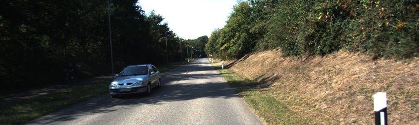
inference time. Depth estimation is performed in stages, during Fig. 1: Example timeline of AnyNet predictions. As time pro-
which the model can be queried at any time to output its gresses the depth estimation becomes increasingly accurate.
current best estimate. Our final model can process 1242×375 The algorithm can be polled at any time to return the current
resolution images within a range of 10-35 FPS on an NVIDIA
Jetson TX2 module with only marginal increases in error – best estimate of the depth map. The initial estimates may be
using two orders of magnitude fewer parameters than the sufficient to trigger an obstacle avoidance maneuver, whereas
most competitive baseline. The source code is available at the later images contain enough detail for more advanced
https://github.com/mileyan/AnyNet. path planning procedures. (3-pixel error rate below time.)
I. INTRODUCTION
Depth estimation from stereo camera images is an impor- on the Nvidia Jetson TX2 GPU computing module — far
tant task for 3D scene reconstruction and understanding, with too slow for timely obstacle avoidance by drones or other
numerous applications ranging from robotics [30], [51], [39], autonomous robots.
[42] to augmented reality [53], [1], [35]. High-resolution In this paper, we argue for an anytime computational
stereo cameras provide a reliable solution for 3D perception approach to disparity estimation, and present a model that
- unlike time-of-flight cameras, they work well both indoors trades off between speed and accuracy dynamically (see
and outdoors, and compared to LiDAR they are substantially Figure 1). For example, an autonomous drone flying at high
more affordable and energy-efficient [29]. Given a rectified speed can poll our 3D depth estimation method at a high
stereo image pair, the focal length, and the stereo baseline frequency. If an object appears in its flight path, it will be
distance between the two cameras, depth estimation can be able to perceive it rapidly and react accordingly by lowering
cast into a stereo matching problem, the goal of which is to its speed or performing an evasive maneuver. When flying at
find the disparity between corresponding pixels in the two low speed, latency is not as detrimental, and the same drone
images. Although disparity estimation from stereo images is could compute a higher resolution and more accurate 3D
a long-standing problem in computer vision [28], in recent depth map, enabling tasks such as high precision navigation
years the adoption of deep convolutional neural networks in crowded scenes or detailed mapping of an environment.
(CNN) [52], [32], [20], [25], [36] has led to significant The computational complexity of depth estimation with
progress in the field. Deep networks can solve the matching convolutional networks typically scales cubically with the
problem via supervised learning in an end-to-end fashion, image resolution, and linearly with the maximum disparity
and they have the ability to incorporate local context as well that is considered [20]. Keeping these characteristics in mind,
as prior knowledge into the estimation process. we refine the depth map successively, while always ensuring
On the other hand, deep neural networks tend to be that either the resolution or the maximum disparity range
computationally intensive and suffer from significant latency is sufficiently low to ensure minimal computation time. We
when processing high-resolution stereo images. For example, start with low resolution (1/16) estimates of the depth map
PSMNet [4], arguably the current state-of-the-art algorithm at the full disparity range. The cubic complexity allows us to
for depth estimation, obtains a frame rate below 0.3FPS compute this initial depth map in a few milliseconds (where
* Authors contributed equally the bulk of the time is spent on the initial feature extraction
1 Cornell University. {yw763, gh349, bhw45, mc288, kqw4}@cornell. and down-sampling). Starting with this low resolution esti-
edu mate, we successively increase the resolution of the disparity
2 University of Oxford. This work performed during Zihang Lai’s
internship at Cornell University. zihang.lai@cs.ox.ac.uk map by up-sampling and subsequently correcting the errors
3 Facebook AI Research. lvdmaaten@gmail.com that are now apparent at the higher resolution. Correction is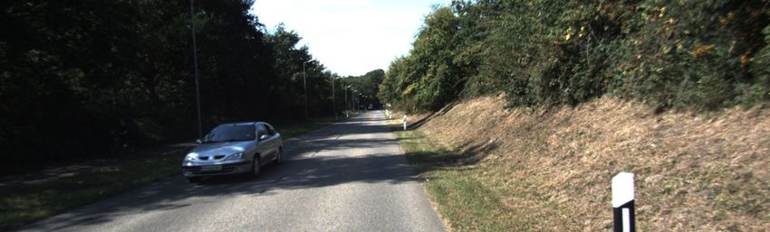
performed by predicting the residual error of the up-sampled         and a convolutional network called DispNet is proposed that
disparity map from the input images with a CNN. Despite              directly predicts disparities for an image pair. Improvements
the higher resolution used, these updates are still fast because     made by DispNet include a cascaded refinement procedure
the residual disparity can be assumed to be bounded within           [36]. Other studies adopt the correlation layer introduced
a few pixels, allowing us to restrict the maximum disparity,         in [7] to obtain the initial matching costs; a set of two
and associated computation, to a mere 10 − 20% of the full           convolutional networks are trained to predict and further
range.                                                               refine the disparity map for the image pair [25]. Several prior
   These successive updates avoid full-range disparity com-          studies have also explored moving away from the supervised
putation at all but the initial low resolution setting, and ensure   learning paradigm by performing depth estimation in an un-
that all computation is re-used, setting our method apart from       supervised fashion using stereo images [9] or video streams
most existing multi-scale network structures [40], [15], [19].       [54].
Furthermore, our algorithm can be polled at any time in                 Our work is partially inspired by the Geometry and Con-
order to retrieve the current best estimated depth map. A            text Network (GCNet) proposed in [20]. In order to predict
wide range of possible frame rates are attainable (10-35FPS          the disparity map between two images, GCNet combines a
on a TX2 module), while still preserving accurate disparity          2D Siamese convolutional network operating on the image
estimation in the high-latency setting. Our entire network can       pair with a 3D convolutional network that operates on the
be trained end-to-end using a joint loss over all scales, and        matching cost tensor. GCNet is trained in an end-to-end
we refer to it as Anytime Stereo Network (AnyNet).                   fashion, and is presently one of the state-of-the-art methods
   We evaluate AnyNet on multiple benchmark data sets                in terms of accuracy and computational efficiency. Our model
for depth estimation, with various encouraging findings:             is related to GCNet in that it has the same two stages (a 2D
Firstly, AnyNet obtains competitive accuracy with state of           Siamese image convolutional network and a 3D cost tensor
the art approaches, while having orders of magnitude fewer           convolutional network), but it differs in that it can perform
parameters than the baselines. This is especially impactful          anytime prediction by rapidly producing an initial disparity
for resource-constrained embedded devices. Secondly, we              map prediction and then progressively predicting the residual
find that deep convolutional networks are highly capable             to correct this prediction. LiteFlowNet [16] also tries to
at predicting residuals from coarse disparity maps. Finally,         predict the residual for optical flow computation. However,
including a final spatial propagation model (SPNet) [26]             LiteFlowNet uses the residual to facilitate large-displacement
significantly improves the disparity map quality, yielding           flow inference rather than computational speedup.
state-of-the-art results at a fraction of the computational cost           c) Anytime prediction: There exists a substantial body
(and parameter storage requirements) of existing methods.            of work on machine learned models with computational bud-
                                                                     get constraints at inference time [46], [10], [18], [49], [50],
                   II. RELATED WORK                                  [47], [15]. Most of these approaches are based on ensembles
      a) Disparity estimation: Traditional approaches to dis-        of decision-tree classifiers [46], [49], [10], [50] which allow
parity estimation are based on matching features between the         for tree-by-tree evaluation, facilitating the progressive pre-
left and right images [2], [41]. These approaches are typically      diction updates that are the hallmark of anytime prediction.
comprised of the following four steps: (1) computing the             Several recent studies have explored anytime prediction with
costs of matching image patches over a range of disparities,         image classification CNNs that dynamically evaluate parts
(2) smoothing the resulting cost tensor via aggregation              of the network to progressively refine their predictions [24],
methods, (3) estimating the disparity by finding a low-cost          [15], [45], [48], [33], [6]. Our work differs from these earlier
match between the patches in the left image and those in             anytime CNN models in that we focus on the structured
the right image, and (4) refining these disparity estimates by       prediction problem of disparity-map estimation, rather than
introducing global smoothness priors on the disparity map            on image classification tasks. Our models exploit particular
[41], [13], [11], [14]. Several recent papers have studied           properties of the disparity-prediction problem: namely, that
the use of convolutional networks in step (1). In particular,        progressive estimation of disparities can be achieved by
Zbontar & LeCun [52] use a Siamese convolutional network             progressively increasing the resolution of the image data
to predict patch similarities for matching left and right            within the internal representation of the CNN.
patches. Their method was further improved via the use of
more efficient matching networks [29] and deeper highway                                     III. A NY N ET
networks trained to minimize a multilevel loss [43].                    Fig. 2 shows a schematic layout of the AnyNet architec-
      b) End-to-end disparity prediction: Inspired by these          ture. An input image pair first passes through the U-Net
initial successes of convolutional networks in disparity esti-       feature extractor, which computes feature maps at several
mation, as well as by their successes in semantic segmen-            output resolutions (of scale 1/16, 1/8, 1/4). In the first
tation [27], optical flow computation [7], [17], and depth           stage, only the lowest-scale features (1/16) are computed and
estimation from a single frame [5], several recent studies           passed through a disparity network (Fig. 4) to produce a low-
have explored end-to-end disparity estimation models [32],           resolution disparity map (Disparity Stage 1). A disparity map
[20], [25], [36]. For example, in [32], the disparity prediction     estimates the horizontal offset of each pixel in the right input
problem is formulated as a supervised learning problem,              image w.r.t. the left input image, and can be used to compute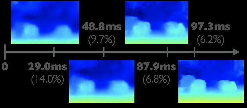
Scale = 1/8

                                    Stage 1
                                                             Disparity
                                                                                                                         Disparity Stage 1   Time
                             1/16                            Network

                   U-Net            Stage 2                                                    Residual 2                Disparity Stage 2
                  Feature                     Warping        Disparity
                             1/8                             Network                                                 +
                 Extractor

                                    Stage 3                                       Residual 3                             Disparity Stage 3
                                              Warping        Disparity
                             1/4                             Network                                         +

                                    Stage 4                                                                              Disparity Stage 4

                                                                                                    SPNet
                  Input
                Image pair
                                                                 Up-sampling           Data flow

                                                        Fig. 2: Network structure of AnyNet.

          Down-sampling                                               1/16
             Up-sampling                                             Feature   images in order to compute a disparity map. We use this
          2D Convolution                                              maps
         Skip connnection                                                      component to compute the initial disparity map (stage 1) as
                1/8
                1/4                                                    1/8
                                                                     Feature
                                                                               well as to compute the residual maps for subsequent correc-
                                                                      maps     tions (stages 2 & 3). The disparity network first computes a
                                                                       1/4     disparity cost volume. Here, the cost refers to the similarity
                                                                     Feature
                                                                      maps     between a pixel in the left image and a corresponding pixel in
 Input image
                                                                               the right image. If the input feature maps are of dimensions
                                                                               H ×W , the cost volume has dimensions H ×W ×M , where
    Fig. 3: U-Net Feature Extractor. See text for details.                     the (i, j, k) entry describes the degree to which pixel (i, j) of
                                                                               the left image matches pixel (i, j−k) in the right image. M
a depth map. Because of the low input resolution, the entire                   denotes the maximum disparity under consideration. We can
Stage 1 computation requires only a few milliseconds. If                       represent each pixel (i, j) in the left image as a vector pL   ij ,
more computation time is permitted, we enter Stage 2 by
                                                                               where dimension α corresponds to the (i, j) entry in the αth
continuing the computation in the U-Net to obtain larger-
                                                                               input feature map associated with the left image. Similarly
scale (1/8) features. Instead of computing a full disparity
                                                                               we can define pR    ij . The entry (i, j, k) in the cost volume is
map at this higher resolution, in Stage 2 we simply correct
                                                                               then defined as the L1 distance between the two vectors pL      ij
the already-computed disparity map from Stage 1. First, we
                                                                               and pR                          L       R
                                                                                      i(j+k) , i.e. Cijk = kpij − pi(j−k) k1 .
up-scale the disparity map to match the resolution of Stage
                                                                                  This cost volume may still contain errors due to blurry
2. We then compute a residual map, which contains small
                                                                               objects, occlusions, or ambiguous matchings in the input
corrections that specify how much the disparity map should
                                                                               images. As a second step in the disparity network (3D
be increased or decreased for each pixel. If time permits,
                                                                               Conv in Fig 4), we refine the cost volume with several 3D
Stage 3 follows a similar process as Stage 2, and doubles the
                                                                               convolution layers [20] to further improve the obtained cost
resolution again from a scale of 1/8 to 1/4. Stage 4 refines
                                                                               volume.
the disparity map from Stage 3 with an SPNet [26].
                                                                                  The disparity for pixel (i, j) in the left image is k if the
   In the remainder of this section we describe the individual
                                                                               pixel (i, j− k) in the right image is most similar. If the cost
components of our model in greater detail.
                                                                               volume is exact, we could therefore compute the disparity
      a) U-Net Feature Extractor: Fig 3 illustrates the U-
                                                                               of pixel (i, j) as D̂ij = argmink Ci,j,k . However, the cost
Net [38] Feature Extractor in detail, which is applied to both
                                                                               estimates may be too noisy to search for the hard minimum.
the left and right image. The U-Net architecture computes
                                                                               Instead, we follow the suggestion by Kendall et al. [20] and
feature maps at various resolutions (1/16, 1/8, 1/4), which
                                                                               compute a weighted average (Disparity regression in Fig 4)
are used as input at stages 1-3 and only computed when
needed. The original input images are down-sampled through                                                  M
                                                                                                            X          exp (−Cijk )
max-pooling or strided convolution and then processed with                                        D̂ij =        k × PM                  .           (1)
                                                                                                                     k0 =0 exp (−Cijk )
                                                                                                                                     0
convolutional filters. Lower resolution feature maps capture                                                k=0

the global context, whereas higher resolution feature maps                     If one disparity k clearly has the lowest cost (i.e. it is the only
capture local details. At scale 1/8 and 1/4, the final convolu-                good match), it will be recovered by the weighted average.
tional layer incorporates the previously computed lower-scale                  If there is ambiguity, the output will be an average of the
features.                                                                      viable candidates.
      b) Disparity Network: The disparity network (Fig. 4)                          c) Residual Prediction: A crucial aspect of our AnyNet
takes as input the feature maps from the left and right stereo                 architecture is that we only compute the full disparity map at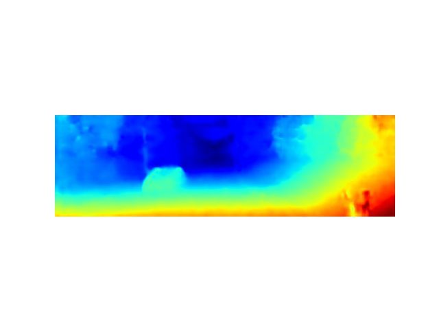
0       Input image
                               3D     Disparity                                                        2-D Unet features
                              Conv   regression   Disparity Residual           1       3×3 conv with 1 filter
  Left/right Distance-based
Feature Maps Cost Volume                          (Stage 1) (Stage 2-3)        2       3×3 conv with stride 2 and 1 filter
                                                                               3       2×2 maxpooling with stride 2
                                                                               4-5     3×3 conv with 2 filters
         Fig. 4: Disparity network. See text for details.                      6       2×2 maxpooling with stride 2
                                                                               7-8     3×3 conv with 4 filters
                                                                               9       2×2 maxpooling with stride 2
a very low resolution in Stage 1. In Stages 2 & 3 we predict                   10-11   3×3 conv with 8 filters
residuals [16]. The most expensive part of the disparity                       12      Bilinear upsample layer 11 (features) into 2x size
                                                                               13      Concatenate layer 8 and 12
prediction is the construction and refinement of the cost                      14-15   3×3 conv with 4 filters
volume. The cost volume scales H × W × M , where M                             16      Bilinear upsample layer 15 (features) into 2x size
                                                                               17      Concatenate layer 5 and 16
is the maximum disparity. In high resolutions, the maximum                     18-19   3×3 conv with 2 filters
disparity between two pixels can be very large (typically                                                 Cost volume
M = 192 pixels in the KITTI dataset [8]). By restricting                       20      Warp and build cost volume from layer 11
                                                                               21      Warp and build cost volume from layer 15 and layer 29
ourselves to residuals, i.e. corrections of existing disparities,              22      Warp and build cost volume from layer 19 and layer 36
we can limit ourselves to M = 5 (corresponding to offsets                                                Regularization
                                                                               23-27   3×3×3 3-D conv with 16 filters
−2, −1, 0, 1, 2) and obtain sizable speedups.                                  28      3×3×3 3-D conv with 1 filter
    In order to compute residuals in stages 2 & 3, we first up-                29      Disparity regression
                                                                               30      Upsample layer 29 to image size: stage 1 disparity output
scale the coarse disparity map and use it to warp the input                    31-35   3×3×3 3-D conv with 4 filters
features at the higher scale (Fig. 2) by applying the disparity                36      Disparity regression: residual of stage 2
                                                                               37      Upsample 36 it into image size
estimations pixel-wise. In particular, if the left disparity of                38      Add layer 37 and layer 30
pixel (i, j) is estimated to be k, we overwrite the value of                   39      Upsample layer 38 to image size: stage 2 disparity output
                                                                               40-44   3×3×3 3-D conv with 4 filters
pixel (i, j) in each right feature map to the corresponding                    45      Disparity regression: residual of stage 3
value of pixel (i, j + k) (using zero if out of bounds). If                    46      Add layer 44 and layer 38
                                                                               47      Upsample layer 46 to image size: stage 3 disparity output
the current disparity estimate is correct, the updated right                                     Spatial propagation network
feature maps should match the left feature maps. Due to the                    48-51   3×3 conv with 16 filters (on input image)
                                                                               52      3×3 conv with 24 filters: affinity matrix
coarseness of the low resolution inputs, there is typically still              53      3×3 conv with 8 filters (on layer 47)
a mismatch of several pixels, which we correct by computing                    54      Spatial propagate layer 53 with layer 52 (affinity matrix)
                                                                               55      3×3 conv with 1 filters: stage 4 disparity output
residual disparity maps. Prediction of the residual disparity is
accomplished similarly to the full disparity map computation.             TABLE I: Network configurations. Note that a conv stands
The only difference is that the cost volume is computed                   for a sequence of operations: batch normalization, rectified
as Cijk = kpij − pi(j−k+2) k1 , and the resulting residual                linear units (ReLU) and convolution. The default stride is 1.
disparity map is added to the up-scaled disparity map from
the previous stage.
       d) Spatial Propagation Network: To further improve                 λ4 = 1, respectively. In total, our model contains 40,000
our results, we add a final fourth stage in which we use                  parameters - this is an order of magnitude fewer parameters
a Spatial Propagation Network (SPNet) [26] to refine our                  than StereoNet [21], and two orders of magnitude fewer
disparity predictions. The SPNet sharpens the disparity map               than PSMNet [4]. Our model is trained end-to-end using
by applying a local filter whose weights are predicted by                 Adam [22] with initial learning rate 5e−4 and batch size
applying a small CNN to the left input image. We show that                6. On the Scene Flow dataset [32], the learning rate is kept
this refinement improves our results significantly at relatively          constant, and the training lasts for 10 epochs in total. For the
little extra cost.                                                        KITTI dataset we first pre-train the model on Scene Flow,
                IV. EXPERIMENTAL RESULTS                                  before fine-tuning it for 300 epochs. The learning rate is di-
   In this section, we empirically evaluate our method and                vided by 10 after epoch 200. All input images are normalized
compare it with existing stereo algorithms. In addition, we               to be zero-mean with unit variance. All experiments were
benchmark the efficiency of our approach on an Nvidia                     conducted using original image resolutions. Using one GTX
Jetson TX2 computing module.                                              1080Ti GPU, training on the Scene Flow dataset took 3.5
     a) Implementation Details: We implement AnyNet in                    hours, and training on KITTI took 30 minutes. All results are
PyTorch [37]. See Table I for a detailed network description.             averaged over five randomized 80/20 train/validation splits.
Our experiments use an AnyNet implementation with four                       Figure 5 visualizes the disparity maps predicted at the four
stages, as shown in Figure 2 and described in the previous                stages of our model. As more computation time is made
section. The maximum disparity is set to 192 pixels in the                available, AnyNet produces increasingly refined disparity
original image, which corresponds to a Stage 1 cost volume                maps. The final output from stage 4 is even sharper and
depth of M = 192/16 = 12. In Stages 2 & 3 the residual                    more accurate, due to the SPNet post-processing.
range is ±2, corresponding to ±16 pixels in Stage 2 and                        b) Datasets: Our model is trained on the synthetic
±8 pixels in Stage 3. All four stages, including the SPNet                Scene Flow [32] dataset and evaluated on two real-world
in Stage 4, are trained jointly, but the losses are weighted              datasets, KITTI-2012 [8] and KITTI-2015 [34]. The Scene
differently, with weights λ1 = 1/4, λ2 = 1/2, λ3 = 1 and                  Flow dataset contains 22, 000 stereo image pairs for train-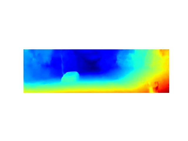
Stage 1       Stage 2      Stage 3       Stage 4
                                                                 Dataset

      (Err=10.4%)
       (a) Stage 1
                                                                            28.9ms       48.8ms       87.9ms        97.3ms
                                                                KITTI2012 15.1 ± 1.1    9.9 ± 0.6    6.7 ± 0.4     6.1 ± 0.3
                                                                KITTI2015 14.0 ± 0.7    9.7 ± 0.7    6.8 ± 0.6     6.2 ± 0.6

                                                               TABLE II: Three-Pixel error (%) of AnyNet on KITTI-2012
                                                               and KITTI-2015 datasets. Lower values are better.
      (b) Stage 2
      (Err=7.5%)

                                                               for faster inference times. The baseline methods are re-
                                                               implemented, and trained on down-sampled stereo images
                                                               - this allows a fair comparison, since a model trained on
      (c) Stage 3
      (Err=5.1%)

                                                               full-sized images would be expected to suffer a significant
                                                               performance decrease when given lower-resolution inputs.
                                                               After obtaining a low-resolution prediction, we up-sample it
                                                               to the original size using bilinear interpolation.
      (d) Stage 4
      (Err=4.2%)

                                                               A. Evaluation Results
                                                                  Table II contains numerical results for AnyNet on the
                                                               KITTI-2012 and KITTI-2015 datasets. Additionally, Figures
      (e) Ground

                                                               6a and 6a demonstrate the evaluation error and inference time
          Truth

                                                               of our model as compared to baseline methods. Baseline
                                                               algorithm results originally reported in [3], [21], [4], [31],
                                                               [44] are shown plotted with crosses. For AnyNet as well
      left Image
       (f) Input

                                                               as the StereoNet and PSMNet baselines, computations are
                                                               performed across multiple down-sampling input resolutions.
                                                               Results are generated from inputs at full resolution as well
                                                               as at 1/4, 1/8, and 1/16 resolution, with lower resolution
Fig. 5: (a)-(d) Disparity prediction from 4 stages of AnyNet   corresponding to faster inference time as shown on Figs. 6a
on KITTI-2015. As a larger computational budget is made        and 6b. As seen in both plots, only AnyNet and StereoNet
available, the prediction is refined and becomes more accu-    are capable of rapid real-time prediction at ≥30 FPS, and
rate. (e) shows the ground truth LiDAR image, and (f) shows    AnyNet obtains a drastically lower error rate on both data
the left input image.                                          sets. AnyNet is additionally capable of running at over 10
                                                               FPS even with full-resolution inputs, and at each possible
ing, and 4, 370 image pairs for testing. Each image has a      inference time range, AnyNet clearly dominates all baselines
resolution of 960 × 540 pixels. As in [20], we train our       in terms of prediction error. PSMNet is capable of producing
model on 512 × 256 patches randomly cropped from the           the most accurate results overall, however this is only true
original images. The KITTI-2012 dataset contains 194 pairs     at computation rates of 1 FPS or slower. We also observe
of images for training and 195 for testing, while KITTI-2015   that the only non-CNN based approach, OpenCV, is not
contains 200 image pairs for each. All of the KITTI images     competitive in any inference time range.
are of size 1242 × 375.                                              a) Anytime setting: We also evaluate AnyNet in the
      c) Baselines: Although state-of-the-art CNN based        anytime setting, in which we can poll the model prema-
stereo estimation methods have been reported to reach 60FPS    turely at any given time t in order to retrieve its most
on a TITAN X GPU [21], they are far from achieving real-       recent prediction. In order to mimic an anytime setting for
time performance on more resource-constrained computing        the baseline OpenCV, StereoNet, and PSMNet models, we
devices such as the Nvidia Jetson TX2. Here, we present a      make predictions successively at increasingly higher input
controlled comparison on a TX2 between our method and          resolutions and execute them sequentially in ascending order
four competitive baseline algorithms: PSMNet [4], Stere-       of size. At time t we evaluate the most recently computed
oNet [21], DispNet [32], and StereoDNN [44]. The PSM-          disparity map. Figures 6c and 6d show the three-pixel error
Net model has two different versions: PSMNet-classic and       rates in the anytime setting. Similarly to the non-anytime
PSMNet-hourglass. We use the former, as it is much more        results, AnyNet obtains significantly more accurate results
efficient than PSMNet-hourglass while having comparable        in the 10-30 FPS range. Furthermore, the times between
accuracy. For StereoNet, we report running times using a       disparity map completions (visualized as horizontal lines
Tensorflow implementation, which we found to be twice as       in Figs. 6c and 6d) are much shorter than for any of the
fast as a PyTorch implementation.                              baselines, reducing the amount of wasted computation if a
   Finally, we also compare AnyNet to two classical stereo     query is issued during a disparity map computation.
matching approaches: Block Matching [23] and Semi-Global
Block Matching [12], supported by OpenCV [3].                  B. Ablation Study
   In order to collect meaningful results for these baseline     In order to examine the impact of various components
methods on the TX2, we use down-sampled input images           of the AnyNet architecture, we conduct an ablation study
30
OpenCV using three variants of our model. The first replaces the U-
25
KITTI2012 Error (%)
AnyNet Net feature extractor with three separated ConvNets without
20 StereoNet
shared weights; the second computes a full-scale prediction
30 FPS
10 FPS
PSMNet
15 at each resolution level, instead of only predicting the resid-
10 ual disparity; while the third replaces the distance-based cost
5 volume construction method with the method in PSMNet [4]
that produces a stack of 2 × M cost volumes. All ablated
0
102 103 variants of our method are trained from scratch, and results
TX2 Inference Time (ms)
from evaluating them on KITTI-2015 are shown in Fig. 7.
(a) KITTI-2012 results across different down- a) Feature extractor: We modify the model’s feature
sampling resolutions extractor by replacing the U-Net with three separate 2D
30
OpenCV
convolutional neural networks which are similar to one
25 another in terms of computational cost. As seen in Fig. 7
KITTI2015 Error (%)
DispNetC
20 StereoDNN (line AnyNet w/o UNet), the errors increase drastically in
AnyNet
30 FPS
10 FPS
15 StereoNet
the first two stages (20.4% and 7.3%). We hypothesize that
10 PSMNet by extracting contextual information from higher resolutions,
the U-Net produces high-quality cost volumes even at low
5
resolutions. This makes it a desirable choice for feature
0
102 103 104 extraction.
TX2 Inference Time (ms)
b) Residual Prediction: We compare our default net-
(b) KITTI-2015 results across different down- work with a variant that refines the disparity estimation
sampling resolutions by directly predicting disparities, instead of residuals, in
30 the second and third stages. Results are shown in Fig. 7
OpenCV
25 (line AnyNet w/o Residual). While this variant is capable
KITTI2012 Error (%)
AnyNet
30 FPS
10 FPS
20 StereoNet of attaining similar accuracy to the original model, the
15
PSMNet evaluation time in the last two stages is increased by a factor
of more than six. This increase suggests that the proposed
10
method to predict residuals is highly efficient at refining
5 coarse disparity maps, by avoiding the construction of large
0
102 103
cost volumes which need to account for a large range of
TX2 Inference Time (ms) disparities.
(c) KITTI-2012 results using the anytime setting
c) Distance-based Cost Volume: Finally, we evaluate
30 the distance-based method for cost volume construction, by
OpenCV comparing it to the method used in PSMNet [4]. This method
25
KITTI2015 Error (%)
AnyNet builds multiple cost volumes without explicitly calculating
30 FPS
10 FPS
20 StereoNet
PSMNet
the distance between features from the left and right images.
15 The results in Fig. 7 (line AnyNet w/o DBCV) show that our
10 distance-based approach is about 10% faster than this choice,
5 indicating that explicitly considering the feature distance
0
leads to a better trade-off between accuracy and speed.
102 103
TX2 Inference Time (ms) V. D ISCUSSION AND C ONCLUSION
(d) KITTI-2015 results using the anytime setting To the best of our knowledge, AnyNet is the first algorithm
Fig. 6: Comparisons of the 3-pixel error rate (%) KITTI- for anytime depth estimation from stereo images. As (low-
2012/2015 datasets. Dots with error bars show accuracies power) GPUs become more affordable and are increasingly
obtained from our implementations. Crosses show values incorporated into mobile computing devices, anytime depth
obtained from original publications. estimation will enable accurate and reliable real-time depth
estimation for a large variety of robotic applications.
16 AnyNet
KITTI2015 Error (%)
14
AnyNet w/o DBCV ACKNOWLEDGMENT
AnyNet w/o Residual
12 AnyNet w/o Unet This research is supported in part by grants from the
10 National Science Foundation (III-1618134, III-1526012,
8
IIS1149882, IIS-1724282, and TRIPODS-1740822), the Of-
fice of Naval Research DOD (N00014-17-1-2175), and the
6
102 Bill and Melinda Gates Foundation. We are thankful for the
TX2 Inference Time (ms)
generous support of SAP America Inc. We thank Camillo J.
Fig. 7: Ablation results as three pixel error on KITTI-2015. Taylor for helpful discussion.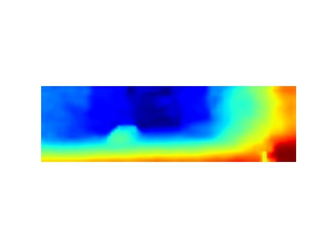
R EFERENCES                                        [27] J. Long, E. Shelhamer, and T. Darrell, “Fully convolutional networks
                                                                                      for semantic segmentation,” in Proceedings of the IEEE conference on
 [1] H. A. Alhaija, S. K. Mustikovela, L. Mescheder, A. Geiger, and                   computer vision and pattern recognition, 2015, pp. 3431–3440.
     C. Rother, “Augmented reality meets computer vision: Efficient data         [28] B. D. Lucas, T. Kanade et al., “An iterative image registration
     generation for urban driving scenes,” International Journal of Com-              technique with an application to stereo vision,” IJCAI, 1981.
     puter Vision, vol. 126, no. 9, pp. 961–972, 2018.                           [29] W. Luo, A. G. Schwing, and R. Urtasun, “Efficient deep learning for
 [2] S. T. Barnard and M. A. Fischler, “Computational stereo,” ACM                    stereo matching,” in CVPR, 2016, pp. 5695–5703.
     Computing Surveys (CSUR), vol. 14, no. 4, pp. 553–572, 1982.                [30] M. Mancini, G. Costante, P. Valigi, and T. A. Ciarfuglia, “Fast
 [3] G. Bradski and A. Kaehler, “Opencv,” Dr. Dobbs journal of software               robust monocular depth estimation for obstacle detection with fully
     tools, vol. 3, 2000.                                                             convolutional networks,” in Intelligent Robots and Systems (IROS),
 [4] J.-R. Chang and Y.-S. Chen, “Pyramid stereo matching network,” in                2016 IEEE/RSJ International Conference on. IEEE, 2016, pp. 4296–
     Proceedings of the IEEE Conference on Computer Vision and Pattern                4303.
     Recognition, 2018, pp. 5410–5418.                                           [31] N. Mayer, E. Ilg, P. Häusser, P. Fischer, D. Cremers, A. Dosovitskiy,
 [5] D. Eigen and R. Fergus, “Predicting depth, surface normals and se-               and T. Brox, “A large dataset to train convolutional networks
     mantic labels with a common multi-scale convolutional architecture,”             for disparity, optical flow, and scene flow estimation,” in IEEE
     in ICCV, 2015.                                                                   International Conference on Computer Vision and Pattern Recognition
 [6] M. Figurnov, M. Collins, Y. Zhu, L. Zhang, J. Huang, D. Vetrov, and              (CVPR), 2016, arXiv:1512.02134. [Online]. Available: http://lmb.
     R. Salakhutdinov, “Spatially adaptive computation time for residual              informatik.uni-freiburg.de/Publications/2016/MIFDB16
     networks,” in CVPR, 2017.                                                   [32] N. Mayer, E. Ilg, P. Hausser, P. Fischer, D. Cremers, A. Dosovitskiy,
 [7] P. Fischer, A. Dosovitskiy, E. Ilg, P. Häusser, C. Hazırbaş, V. Golkov,        and T. Brox, “A large dataset to train convolutional networks for
     P. Van der Smagt, D. Cremers, and T. Brox, “Flownet: Learning optical            disparity, optical flow, and scene flow estimation,” in Proceedings of
     flow with convolutional networks,” arXiv preprint arXiv:1504.06852,              the IEEE Conference on Computer Vision and Pattern Recognition,
     2015.                                                                            2016, pp. 4040–4048.
 [8] A. Geiger, P. Lenz, and R. Urtasun, “Are we ready for autonomous            [33] M. McGill and P. Perona, “Deciding how to decide: Dynamic routing
     driving? the kitti vision benchmark suite,” in Conference on Computer            in artificial neural networks,” in arXiv:1703.06217, 2017.
     Vision and Pattern Recognition (CVPR), 2012.                                [34] M. Menze and A. Geiger, “Object scene flow for autonomous ve-
 [9] C. Godard, O. Mac Aodha, and G. J. Brostow, “Unsupervised monoc-                 hicles,” in Conference on Computer Vision and Pattern Recognition
     ular depth estimation with left-right consistency,” CVPR, vol. 2, no. 6,         (CVPR), 2015.
     p. 7, 2017.                                                                 [35] C. Nguyen, S. DiVerdi, A. Hertzmann, and F. Liu, “Depth conflict
[10] A. Grubb and D. Bagnell, “Speedboost: Anytime prediction with                    reduction for stereo vr video interfaces,” in Proceedings of the 2018
     uniform near-optimality.” in AISTATS, vol. 15, 2012, pp. 458–466.                CHI Conference on Human Factors in Computing Systems. ACM,
[11] H. Hirschmuller and D. Scharstein, “Evaluation of stereo matching                2018, p. 64.
     costs on images with radiometric differences,” TPAMI, vol. 31, pp.          [36] J. Pang and W. Sun, “Cascade residual learning: A two-stage con-
     1582–1599, 2009.                                                                 volutional neural network for stereo matching,” in arXiv:1708.09204,
[12] H. Hirschmuller, “Stereo processing by semiglobal matching and                   2017.
     mutual information,” IEEE Transactions on pattern analysis and              [37] A. Paszke, S. Gross, S. Chintala, G. Chanan, E. Yang, Z. DeVito,
     machine intelligence, vol. 30, no. 2, pp. 328–341, 2008.                         Z. Lin, A. Desmaison, L. Antiga, and A. Lerer, “Automatic differen-
[13] A. Hosni, C. Rhemann, M. Bleyer, C. Rother, and M. Gelautz, “Fast                tiation in pytorch,” 2017.
     cost-volume filtering for visual correspondence and beyond,” TPAMI,         [38] O. Ronneberger, P. Fischer, and T. Brox, “U-net: Convolutional
     vol. 35, pp. 504–511, 2013.                                                      networks for biomedical image segmentation,” in International Confer-
[14] X. Hu and P. Mordohai, “A quantitative evaluation of confidence                  ence on Medical image computing and computer-assisted intervention.
     measures for stereo vision,” TPAMI, vol. 34, pp. 2121–2133, 2012.                Springer, 2015, pp. 234–241.
[15] G. Huang, D. Chen, T. Li, F. Wu, L. van der Maaten, and K. Q.               [39] A. Saxena, J. Schulte, A. Y. Ng et al., “Depth estimation using
     Weinberger, “Multi-scale dense convolutional networks for efficient              monocular and stereo cues.” in IJCAI, vol. 7, 2007.
     prediction,” in ICLR, 2017.                                                 [40] S. Saxena and J. Verbeek, “Convolutional neural fabrics,” in NIPS,
[16] T.-W. Hui, X. Tang, and C. C. Loy, “Liteflownet: A lightweight con-              2016, pp. 4053–4061.
     volutional neural network for optical flow estimation,” in Proceedings      [41] D. Scharstein and R. Szeliski, “A taxonomy and evaluation of dense
     of IEEE Conference on Computer Vision and Pattern Recognition                    two-frame stereo correspondence algorithms,” International journal of
     (CVPR), June 2018, pp. 8981–8989.                                                computer vision, vol. 47, no. 1-3, pp. 7–42, 2002.
[17] E. Ilg, N. Mayer, T. Saikia, M. Keuper, A. Dosovitskiy, and T. Brox,        [42] K. Schmid, T. Tomic, F. Ruess, H. Hirschmüller, and M. Suppa,
     “Flownet 2.0: Evolution of optical flow estimation with deep net-                “Stereo vision based indoor/outdoor navigation for flying robots,” in
     works,” in CVPR, 2017.                                                           Intelligent Robots and Systems (IROS), 2013 IEEE/RSJ International
[18] S. Karayev, M. Fritz, and T. Darrell, “Anytime recognition of objects            Conference on. IEEE, 2013, pp. 3955–3962.
     and scenes,” in CVPR, 2014, pp. 572–579.                                    [43] A. Shaked and L. Wolf, “Improved stereo matching with constant
[19] T. Ke, M. Maire, and S. X. Yu, “Neural multigrid,” CoRR, vol.                    highway networks and reflective confidence learning,” in CVPR, 2017.
     abs/1611.07661, 2016. [Online]. Available: http://arxiv.org/abs/1611.       [44] N. Smolyanskiy, A. Kamenev, and S. Birchfield, “On the importance of
     07661                                                                            stereo for accurate depth estimation: An efficient semi-supervised deep
[20] A. Kendall, H. Martirosyan, S. Dasgupta, P. Henry, R. Kennedy,                   neural network approach,” arXiv preprint arXiv:1803.09719, 2018.
     A. Bachrach, and A. Bry, “End-to-end learning of geometry and               [45] A. Veit and S. Belongie, “Convolutional networks with adaptive
     context for deep stereo regression,” in ICCV, 2017.                              computation graphs,” in arXiv:1711.11503, 2017.
[21] S. Khamis, S. Fanello, C. Rhemann, A. Kowdle, J. Valentin, and              [46] P. Viola and M. Jones, “Robust real-time object detection,” Interna-
     S. Izadi, “Stereonet: Guided hierarchical refinement for real-time edge-         tional Journal of Computer Vision, vol. 4, no. 34–47, 2001.
     aware depth prediction,” arXiv preprint arXiv:1807.08865, 2018.             [47] J. Wang, K. Trapeznikov, and V. Saligrama, “Efficient learning by
[22] D. P. Kingma and J. Ba, “Adam: A method for stochastic optimiza-                 directed acyclic graph for resource constrained prediction,” in NIPS,
     tion,” arXiv preprint arXiv:1412.6980, 2014.                                     2015, pp. 2152–2160.
[23] K. Konolige, “Small vision systems: Hardware and implementation,”           [48] Z. Wu, T. Nagarajan, A. Kumar, S. Rennie, L. Davis, K. Grauman, and
     in Robotics research. Springer, 1998, pp. 203–212.                               R. Feris, “Blockdrop: Dynamic inference paths in residual networks,”
[24] G. Larsson, M. Maire, and G. Shakhnarovich, “Fractalnet: Ultra-deep              in arXiv:1711.08393, 2017.
     neural networks without residuals,” in ICLR, 2017.                          [49] Z. Xu, K. Q. Weinberger, and O. Chapelle, “The greedy miser:
[25] Z. Liang, Y. Feng, Y. Guo, H. Liu, L. Qiao, W. Chen, L. Zhou, and                Learning under test-time budgets,” in ICML, 2012, pp. 1175–1182.
     J. Zhang, “Learning deep correspondence through prior and posterior         [50] Z. Xu, M. Kusner, M. Chen, and K. Q. Weinberger, “Cost-sensitive
     feature constancy,” arXiv preprint arXiv:1712.01039, 2017.                       tree of classifiers,” in ICML, vol. 28, 2013, pp. 133–141.
[26] S. Liu, S. De Mello, J. Gu, G. Zhong, M.-H. Yang, and J. Kautz,             [51] M. Ye, E. Johns, A. Handa, L. Zhang, P. Pratt, and G.-Z. Yang, “Self-
     “Learning affinity via spatial propagation networks,” in Advances in             supervised siamese learning on stereo image pairs for depth estimation
     Neural Information Processing Systems, 2017, pp. 1520–1530.                      in robotic surgery,” arXiv preprint arXiv:1705.08260, 2017.
[52] J. Zbontar and Y. LeCun, “Stereo matching by training a convolutional
neural network to compare image patches,” Journal of Machine
Learning Research, vol. 17, no. 1-32, p. 2, 2016.
[53] N. Zenati and N. Zerhouni, “Dense stereo matching with application to
augmented reality,” in Signal processing and communications, 2007.
ICSPC 2007. IEEE international conference on. IEEE, 2007, pp.
1503–1506.
[54] T. Zhou, M. Brown, N. Snavely, and D. G. Lowe, “Unsupervised
learning of depth and ego-motion from video,” CVPR, vol. 2, no. 6,
p. 7, 2017.You can also read