Optimal Team Economic Decisions in Counter-Strike
←
→
Page content transcription
If your browser does not render page correctly, please read the page content below
Optimal Team Economic Decisions in Counter-Strike

                                                                        Peter Xenopoulos1 , Bruno Coelho1 , Claudio Silva1
                                                                                      1
                                                                                        New York University
                                                                            {xenopoulos, bruno.coelho, csilva}@nyu.edu
arXiv:2109.12990v1 [cs.GT] 20 Sep 2021

                                                                   Abstract                                     A common approach to valuing players is through the use
                                                                                                             of win probability models. As players perform actions in a
                                              The outputs of win probability models are often                CSGO round, they change their team’s probability of win-
                                              used to evaluate player actions. However, in some              ning that round. We can value players through the cumula-
                                              sports, such as the popular esport Counter-Strike,             tive value of their actions [Xenopoulos et al., 2020]. While
                                              there exist important team-level decisions. For ex-            evaluating players in CSGO is important for teams, fans and
                                              ample, at the beginning of each round in a Counter-            leagues alike, there exist many team-level actions that are im-
                                              Strike game, teams decide how much of their in-                portant to value. For example, at the beginning of each CSGO
                                              game dollars to spend on equipment. Because the                round, two teams asymmetrically determine how much of
                                              dollars are a scarce resource, different strategies            their in-game money to spend on in-game equipment. Given
                                              have emerged concerning how teams should spend                 the current game situation, such as the scores between the
                                              in particular situations. To assess team purchas-              teams, as well as each team’s current equipment value and
                                              ing decisions in-game, we introduce a game-level               money, a team will decide how much of their money to spend.
                                              win probability model to predict a team’s chance
                                                                                                                Teams consider several different spending strategies de-
                                              of winning a game at the beginning of a given
                                                                                                             pending on the game scenario. For example, some teams may
                                              round. We consider features such as team scores,
                                                                                                             elect to “save” for a round, meaning they limit how much in-
                                              equipment, money, and spending decisions. Us-
                                                                                                             game money they spend. On the other hand, some teams may
                                              ing our win probability model, we investigate op-
                                                                                                             “half buy”, meaning they spend some of their money, but still
                                              timal team spending decisions for important game
                                                                                                             retain some dollars for future rounds. The relative outcomes
                                              scenarios. We identify a pattern of sub-optimal
                                                                                                             of the different strategies on win probability are unknown,
                                              decision-making for CSGO teams. Finally, we in-
                                                                                                             since there are many factors to consider, such as team scores,
                                              troduce a metric, Optimal Spending Error (OSE),
                                                                                                             equipment values and team money. Furthermore, current win
                                              to rank teams by how closely their spending deci-
                                                                                                             probability models are tailored towards round-level win prob-
                                              sions follow our predicted optimal spending deci-
                                                                                                             ability, whereas teams are making decisions with game-level
                                              sions.
                                                                                                             win probability in mind.
                                                                                                                In this paper, we introduce a game-level win probability
                                                                                                             model using features such as team scores, team equipment
                                         1   Introduction                                                    values and total team money. We consider various models,
                                                                                                             such as tree-based models and neural networks, and compare
                                         While traditional sports, such as basketball or soccer, have        their performance to a logistic regression baseline. Then, we
                                         embraced data to analyze and value players, esports, also           use these win probability models to assess the optimal spend-
                                         known as professional video gaming, still lags behind. Ex-          ing decisions for various CSGO scenarios. We identify im-
                                         panded data acquisition methods, such as player-worn sensors        portant game situations where the CSGO community is mak-
                                         or cameras that track player movement, typically have driven        ing sub-optimal decisions. Additionally, we introduce Opti-
                                         analytical efforts in a sport. However, esports is unique in that   mal Spending Error (OSE), a metric to measure how much a
                                         many player actions and trajectories are recorded by a game         team’s spending decisions deviate from optimal ones.
                                         server. In many esports, like Counter-Strike: Global Of-               We structure the paper as follows. In section 2, we cover
                                         fensive (CSGO), a popular round-based first person shooter          literature on win probability and valuation frameworks for es-
                                         (FPS), game server logs are written to a demofile. Because          ports. Then, in section 3, we describe CSGO as game, as well
                                         CSGO demofiles are easier to obtain and parse than demofiles        as how CSGO data is collected. Section 4 describes our data
                                         from other esports, CSGO represents a promising direction           and win probability problem formulation, along with the per-
                                         for esports analytics, particularly in player and team valua-       formance of our candidate models. Next, in section 5, we dis-
                                         tion.                                                               cover the optimal spending decisions in various CSGO sce-
                                             Accepted to IJCAI 2021 AISA Workshop                            narios, as well as introduce our OSE metric. Finally, we dis-
cuss limitations, future work and conclude the paper in sec-
tion 6.
2 Related Work
Predicting the chance that a team will win a game is an impor-
tant task in sports analytics. The models used to predict who
will win a game are typically called win probability models, Figure 1: Teams earn $3,250 per player for winning a round, or
and often use the current state of a game as input. From these $3,500 if they successfully detonate the bomb. When a team loses
win probability models, we can assess the value of player ac- a round, they gain a variable amount of money (“loss bonus”) that
tions and decisions. For example, Yurko et al. value Ameri- depends on how many rounds they have lost since they last won a
can football players by how their actions change their respec- round. After each win, the loss bonus resets. Because the money
from losing can be small, teams often find themselves in situations
tive team’s chance of winning the game [Yurko et al., 2019]. where they must determine how much money to invest to maximize
Likewise, Decroos et al. value soccer players by observing their chance of winning the game.
how their actions chance their team’s chance of scoring [De-
croos et al., 2019]. Valuing actions and decisions through
changes in a team’s chance of winning and scoring is com- and player-level analysis. Our work differs in that we predict
mon among contemporary sports, such as in ice hockey [Luo game-level win probability, and we analyze team decisions
et al., 2020; Liu and Schulte, 2018], basketball [Sicilia et and actions, rather than those from players.
al., 2019; Cervone et al., 2014], or soccer [Fernández et al.,
2019]. 3 Counter-Strike
With new data acquisition pipelines, esports has also
started to develop a win probability estimation and player 3.1 Game Rules
valuation literature. Yang et al. built a model to predict Counter-Strike: Global Offensive (CSGO) is the latest rendi-
the winning team in Defense of the Ancients 2 (DOTA2), a tion in the popular Counter-Strike series of video games. In
popular massively online battle arena (MOBA) esport video a professional CSGO match, two teams first meet to decide
game [Yang et al., 2017]. They consider a combination of of what maps, or virtual worlds, they plan on playing. Usually,
pre-match features, as well as real-time features, as input to games are structured as a best-of-three, and the two teams go
a logistic regression model. Semenov et al. use pre-match through a picking and banning process to choose maps they
hero draft information to predict winners in DOTA2 [Se- want to play. There are seven maps used in professional play,
menov et al., 2016]. Hodge et al. parse DOTA2 game re- and the pool of seven maps changes occasionally. Teams win
plays, not only those from professional matches, but those a map when they win 16 rounds, unless the score is 15 for
of very high ranked public players, to predict outcomes in each team; then, an overtime process takes place.
DOTA2 [Hodge et al., 2017]. Later, they also create a live win When teams begin to play a map, they are first assigned to
prediction model for DOTA2 using an ensemble of various either the Terrorists (T) or the Counter-Terrorists (CT). They
machine learning techniques, such as logistic regression, ran- then play for 15 rounds as their assigned side, and the two
dom forests and gradient boosted trees [Hodge et al., 2019]. teams switch sides after 15 rounds. Each round lasts slightly
Recently, Kim et al. propose a confidence calibration method under two minutes. Teams can achieve a variety of round win
for predicting winners in League of Legends, a similar style conditions based on their current side. The T side can win a
game to DOTA2 [Kim et al., 2020]. Yang et al. introduce an round by eliminating all CT players, or by planting a bomb
interpretable model architecture to analyze win predictions in and having it defuse at one of two designated bomb sites. At
Honor of Kings, another popular MOBA game [Yang et al., the beginning of each round, a random T player starts with
2020]. Wang et al. provide a framework to jointly model the bomb. When the bomb is planted, a timer for 35 seconds
win probability and player performance in Fever Basketball, starts counting down. The CT side can win a round by elimi-
a popular sports game [Wang et al., 2020]. nating all T players, defusing a planted bomb, or allowing the
While MOBA games have attracted increasing interest round time to run out, without reaching any of the aforemen-
for win prediction and player valuation, first-person shoot- tioned win conditions.
ers (FPS), such as Counter-Strike, have received less atten- Players begin a round with 100 health points (HP) and are
tion. Makarov et al. predict round winners in CSGO in eliminated when their HP reaches zero. Players lose HP when
post-plant scenarios using decision trees and logistic regres- they are damaged by gunfire or grenades from other players.
sion [Makarov et al., 2017]. Bednarek et al. values play- At the beginning of each round, players can use money earned
ers by clustering death locations, however, they do not create from previous rounds to buy guns, armor, grenades and other
a win prediction model [Bednárek et al., 2017b]. Recently, equipment. Players earn money by eliminating other players
Xenopoulos et al. introduce a player valuation framework and through completing objectives. If a team wins a round,
that uses changes in a team’s win probability to value play- each member gains $3,250 in-game money. However, if a
ers [Xenopoulos et al., 2020]. They model a team’s chance team loses, their monetary gain is based on how many previ-
of winning a CSGO round using XGBoost with input fea- ous rounds they have lost since their last win. For example,
tures such as a team’s remaining players and total equipment. if a team lost the previous round, but won two rounds ago,
Prior CSGO work has focused on round-level win probability they only earn $1,400. We show an example of the variableBuy Type Equipment Spend Win %
Eco 0 – 3k 0 – 2k 3%
Low Buy 0 – 3k 2k – 7.5k 27%
Half Buy 0 – 3k 7.5k – 20k 34%
Hero Low Buy 3k – 20k 0 – 7.5k 25%
Hero Half Buy 3k – 20k 7.5k – 17k 48%
Full Buy Equip. + Spend > 20k+ 59%
Table 1: Teams use different buying strategies depending on their
current money, and which strategy they think will improve their
chance of winning the game. We also report the average round win
rates for each buy type.
“loss bonus” in Figure 1. Since the loss bonus can be mini-
mal, teams often use strategies, known as buy types, to guide
their in-game economic decisions. Some buy types include
deciding not to buy any equipment in a round (referred to as
an “eco”), or buying cheap guns (“low buy” or “half buy”)
in an effort to save money while maximizing their chance
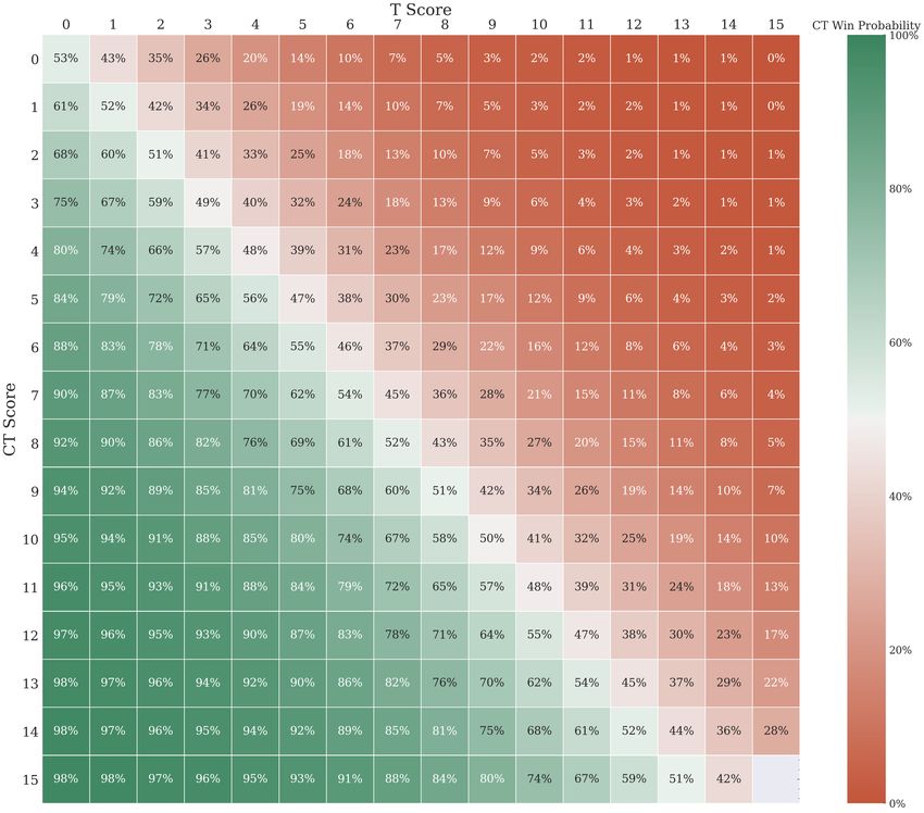
of winning the game. If a player saves equipment from a Figure 2: CT win probability by score on the map Inferno from our
previous round, but the team elects to either eco or half buy, baseline logistic regression model that uses team scores. Winning
they these are referred to as “hero” buys. Finally, if a team’s the first two rounds can increase a team’s chance of winning the
starting equipment value, plus their round monetary spend, is game by roughly 15%.
$20,000 or greater, the team’s buy is referred to as a full buy.
We define the main buy types in Table 1.
Past win probability works have considered a variety
3.2 Data Acquisition of models. For example, logistic regression and gradient
CSGO games take place on a game server, to which the clients boosted trees are often used to model win probability, par-
(players) connect. Each client persists a local game state, con- ticularly because they provide good performance and allow
taining information such as where other players are standing, for easy interpretability measures [Makarov et al., 2017;
team scores and so on. When a client performs some input Decroos et al., 2019; Yang et al., 2017; Semenov et al.,
that changes the game, that input is sent to the game server 2016]. At the same time, neural network approaches are
which then reconciles the global game state across all con- relatively untested for win probability prediction, particu-
nected clients. As the game server updates the global game larly in esports. Therefore, we consider three modeling tech-
state, and sends it to each client, the game server also writes niques: (1) logistic regression, (2) XGBoost, and (3) neu-
the change to a demofile [Bednárek et al., 2017a]. Demofiles ral networks [Chen and Guestrin, 2016]. Logistic regression
are limited to a single map, so for a best-of-three game, at serves as our baseline model, and we show the predicted game
minimum, two demofiles are generated. One can parse a de- win probabilities given different score combinations on the
mofile into a JSON format using a demo parser [Xenopoulos Inferno map in Figure 2. We use the default parameters for
et al., 2020]. logistic regression and fine tune the parameters of the other
model as described in Section 4.2. We train a separate model
4 Modeling Win Probability for each of the seven competitive maps in CSGO, as well as a
In previous win probability works, the objective is typically model where we one-hot encode the map as a feature, denoted
a regression problem starting with a game state Gr,t , which “OHE Map”. We evaluate each model by using log-loss, de-
encapsulates the game information, such as player locations, fined as
equipment values and so on, in round r at time t [Xenopoulos
et al., 2020]. Using this aforementioned game state, the goal
N −1 K−1
is to estimate P (Yr = 1|Gr,t ), where Yr is 1 if the CT side 1 X X
wins round r and 0 otherwise. We vary from this formulation − yi,k log pi,k (1)
N i=0
by instead considering Rg,i , which is the game information k=0
at the start of round i for game g. We can represent Rg,i as
a vector including each side’s current score, the difference in where K is the number of labels, N is the number of ob-
score, each side’s starting equipment value and money, and servations. Each model’s log-loss on the test set is shown in
the buy decisions for both sides in round i. Using Rg,i , we Table 2. While more complex models, like XGBoost and neu-
want to estimate P (Yg |Rg,i ), where Yg represents the game ral networks, clearly outperform our logistic regression base-
outcome decision for game g. Yg can represent three unique line, the performance differences between XGBoost and our
values: (1) the game is won by the current CT side, (2) the neural network are minimal. We found a small performance
current T side, or (3) the game ends in a draw. benefit to using one-hot encoding for the map feature.Logistic Neural Model Hyperparameter Lower Upper Step
Map Rounds XGBoost
Regression Network Learning rate 0.05 0.31 0.05
dust2 8144 0.820 0.766 0.767 Max depth 3 10 1
XGBoost
inferno 10508 0.769 0.708 0.709 Min. child weight 1 8 1
mirage 7712 0.876 0.827 0.830 Colsample 0.3 0.8 0.1
nuke 8266 0.773 0.716 0.716 Dense 1 16 128 16
overpass 6230 0.717 0.673 0.660 Dense 2 16 128 16
NN
train 7565 0.824 0.767 0.766 Dropout 0.1 0.6 0.1
vertigo 6080 0.768 0.710 0.707 Learning rate 10−3 10−5 0.1*
Weighted Average 0.793 0.739 0.736
Table 3: Range of values and step sizes considered for each hyper-
OHE Map - 0.730 0.732 parameter. For the learning rate of the neural network, we instead
use a exponential step increment and multiply each value by 0.1.
Table 2: Log-loss results by map for each of our candidate models.
The logistic regression baseline uses only team scores. The tuned
XGBoost model and the tuned neural network have similar results,
with the neural network having a slightly smaller weighted average explored for each hyperparameter. We use the same range for
loss. Using map as a feature, instead of a separate model for each both tuning a model per map and for the OHE Map models.
map, performs slightly better.
5 Discussion
4.1 Data 5.1 Investigating Common Buy Strategies
We use 6,538 demofiles from matches between April 1st,
2020 to April 20th, 2021. We use this time period as all One benefit of our approach is that we can estimate the game
matches were played online, however, for matches before win probability for a variety of possible buy types. We would
April 2020, it was common for matches to be played on lo- expect that different buys should naturally change a team’s
cal area networks, where players were in the same room to probability of winning a game. We show the effects of dif-
lower game server ping. Liu et al. find that lower latencies ferent buys on predicted team win probability in Figure 3. In
can drastically affect player performance [Liu et al., 2021]. doing so, we can determine the optimal buy type for a side
Therefore, matches held in LAN tournaments versus those in a given round by observing which buy type maximizes a
held online may not be directly comparable. We acquired team’s game win probability. We present a confusion matrix
our demofiles from the popular CSGO fan site, HLTV.org. in Table 4 which shows the optimal buy types, along with
For training, we use matches from April 1st, 2020 to the the actual performed buy types for each side. While some
end of September 2020 (3,308 demofiles), for validation, we buy types are overwhelmingly taken when optimal, such as
use matches from October and November 2020 (1,108 de- the Full Buy, others, like an Eco buy, are performed more of-
mofiles), and finally, for testing, we use matches from De- ten than is predicted optimal. For example, out of the nearly
cember 1st, 2020 to April 20th, 2021 (2,122 demofiles). 2,000 rounds where CT side performed an Eco buy, the pre-
dicted optimal buy was either a Low or Half buy, in over 90%
of rounds, leading to an average lost win probability of about
4.2 Hyperparameter Tuning 3%.
For XGBoost, we use the Hyperopt [Bergstra et al., 2013] The first few rounds of any CSGO game are crucial for
optimization library with default parameters to fine-tune the both sides. As we see from Figure 2, by winning the first
learning rate, maximum tree depth, minimum child weight two rounds, the CT side achieves a 68% game win rate on
and the subsample ratio of columns for each level. We use the Inferno map. Such a high game win rate for winning the
the validation set indicated in Section 4.1. On the final model first two rounds is standard across all maps. The side which
we use early stopping on the validation loss with a patience loses the first round must then decide what their buy type will
of 10 iterations to also tune the number of boosting rounds. be for the second round. Almost always, the possible buys
For the neural network, we create a two-layer fully- will be an eco, low buy or half buy. The rational behind half
connected network, where each layer has a ReLU activation buying is that the team which won the first round will still not
function and dropout applied [Srivastava et al., 2014]. We have the best equipment available, thus by half buying, they
base our two-layer design choice on the work of Yurko et al. , will have a better chance of winning the second round and
where they considered a two layer fully-connected network to forcing their opponents to have a low loss bonus. However, if
predict an American football ball carrier’s end position as one a team chooses to eco, they may save more money to spend in
of their candidate models [Yurko et al., 2020]. We fine-tune the third or fourth rounds. In Table 5, we show the buy rates
the amount of hidden units in each layer, the dropout proba- by side for second rounds where a team lost the first round.
bility and the learning rate using random search and use early It is clear that in general, opting to half buy in the second
stopping with a patience of 10 epochs on the final model. Our round is a popular strategy, but in almost 40% of rounds, the
output layer contains three units, one for a CT win, T win and T side will either eco or low buy. At the same time, our model
draw, the three possible game outcomes, to which we apply a overwhelmingly predicts that a team should half buy in the
softmax activation function. In Table 3 we specify the range second if they lose the first.ACTUAL
O CT Eco Low Buy Half Buy Hero Low Buy Hero Half Buy Full Buy
P Eco 47 136 141 0 0 756
T Low Buy 258 270 1218 0 0 2880
I Half Buy 1675 2126 3557 0 0 2173
M Hero Low Buy 0 0 0 680 86 1081
A Hero Half Buy 0 0 0 1926 568 4453
L Full Buy 3 86 114 31 29 25967
ACTUAL
O T Eco Low Buy Half Buy Hero Low Buy Hero Half Buy Full Buy
P Eco 20 23 26 0 0 1
T Low Buy 174 706 1647 0 0 1378
I Half Buy 1582 2283 4726 0 0 157
M Hero Low Buy 0 0 0 159 247 1794
A Hero Half Buy 0 0 0 241 196 4225
L Full Buy 0 63 623 30 13 29946
Table 4: Confusion matrices of predicted optimal side buy types and actual side buy types for our test set. We see that in many instances, the
predicted optimal buy type differs from the actual buy type, particularly for eco and low buy situations.
5.2 Assessing Team Economic Decisions
Aside from observing community-wide team buy tendencies,
we can also rank teams by how well their buys correlate with
the optimal ones determined from our model. To that effect,
we introduce Optimal Spending Error, defined as
X
OSET = (WT,r − OT,r )2 (2)
r∈RT
which is the mean-squared error between the predicted win
probability, and the optimal buy win probability, for team T
across all rounds which team T plays, denoted RT . Thus,
teams with low OSEs are making economic decisions in line
with what our model predicts as optimal. We calculate OSE
for all teams in our test set, and report the results for teams
ranked in the top 50 in Table 6. We see that in general teams
with a top HLTV ranks have low OSEs, although the relation-
ship is not completely captured by HLTV ranks, since teams
Figure 3: The estimated win probability for each side in the first half experience different tiers of competition not delineated in the
of a game on the Inferno map. We show two alternate buys, one data. For example, a top 50 team is not often playing against a
where buying less (Eco instead of Half Buy) would have decreased team ranked below the top 50. Therefore, we consider the re-
the T’s chance of winning, and one where buying more (Hero Half lationship between a team’s round win rate and their OSE. We
Buy instead of Hero Low Buy) would have decreased the T’s chance would expect that teams which attain low OSEs, and therefore
of winning.
make optimal buy decisions, would also have high round win
rates. We confirm this relationship between team OSE and
round win rates in Figure 4. We find a slight (r = −0.45) re-
Low Half lationship between team OSE and round win rate, indicating
Eco
Buy Buy that teams with higher OSEs have lower round win rates.
T 27% 10% 63%
Actual
CT 6% 3% 91% 5.3 Accounting for New Maps
T 0% 0% 100%
Optimal One interesting consideration is understanding how our mod-
CT 4% 0% 96%
els behave when a new map is added to the Active Duty
Table 5: Actual and optimal buy type rates, by side, for second Group, which is the list of active competitive maps. To study
rounds where the team lost the first (pistol) round. Our model pre- the generalization abilities of our models, we train a neural
dicts that half buy is the most optimal buy type in most situations, network with no map features on six out of the seven avail-
increasing able maps, and then evaluate the test loss on the held out map,
imitating a scenario where a brand new map is introduced.Top 5 Bottom 5
Average CT T HLTV Average CT T HLTV
Team Team
OSE OSE OSE Rank OSE OSE OSE Rank
FPX 0.00024 0.00043 0.00005 16 ENCE 0.00352 0.00501 0.00178 26
Gambit 0.00133 0.00090 0.00114 1 HAVU 0.00309 0.00348 0.00271 14
SKADE 0.00141 0.00114 0.00165 23 Liquid 0.00306 0.00312 0.00300 8
Copenhagen
Dignitas 0.00160 0.00143 0.00176 25 0.00265 0.00387 0.00155 33
Flames
NIP 0.00176 0.00122 0.00230 13 Anonymo 0.00247 0.00264 0.00229 47
Table 6: Top and Bottom 5 teams by OSE. Only teams in the Top 50 HLTV.org rankings on April 26th, 2021, and have played at least 300
rounds in our test set, are included.
Previous
Held out map Initial model Fine Tuned
best NN
dust2 0.767 0.759 0.761
inferno 0.709 0.715 0.705
mirage 0.830 0.821 0.822
nuke 0.716 0.718 0.716
overpass 0.660 0.646 0.646
train 0.766 0.768 0.759
vertigo 0.707 0.697 0.695
Table 7: Log-loss results by map for our previous hyperparameter
tuned models, a initial model which was trained with data from all
other maps and one that was fine tuned on the held out map. The
maps trained on more data, either before or after fine-tuning per-
form better in 6 out of 7 cases indicating there is little advantage to
Figure 4: Teams with a high Optimal Spending Error (OSE), which training a model on a specific map only.
translates into more sub-optimal team economic decision making,
typically have lower round win rates (r = −0.45).
We then investigate team buying decisions across the profes-
We maintain the neural network architecture described in sional CSGO community. We find that teams are much more
section 4.2 and use 96 and 32 neurons for the first and second conservative with respect to round buying decisions than our
layer respective, 0.1 dropout probability and a learning rate model predicts is optimal. Particularly in second rounds,
of 10−4 with no hyperparameter tuning. We then fine tune where a team lost the first round of the game, many teams
our model with a lower learning rate of 10−5 on the new map are making sub-optimal buy decisions on the T side, with
and observe the new test loss. Table 7 shows the loss for each respect to our model. We also introduce Optimal Spending
map, where we also repeat the neural network results from Error (OSE), a metric to assess a team’s economic decision
Table 2 for easier comparison. We observe that both the initial making. We find that OSE is correlated with other team suc-
models and the fine tuned models perform better or equal to cess measures, such as round win rate. Finally, we conduct a
our previous neural network trained on a specific map only, test to assess how our model performs for “unplayed” maps,
showing that for our problem the amount of data available or maps that are not part of the active map pool. We find that
for the model is more helpful than explicitly capturing effects our models can easily generalize to win probability prediction
of a specific map. This agrees with our previous results in on new maps.
Table 2 where the OHE model had a lower average loss than We see many avenues of future work. One of the limi-
the individual per map models across both neural networks tations of our work is that our data is limited to organized
and XGBoost. Thus, for future additions to the map pool, semi-professional and professional games. Because these
we can consider a model which uses no map information to games often have teams with dedicated, oftentimes very sim-
achieve a rough win probability estimate. ilar, strategies for particular scenarios, in some cases there
may not be much variation buy types. Consider the exam-
ple in Table 5. While there is variation in T buys for second
6 Conclusion rounds, the CT round buys have a high imbalance. One way
This work introduces a game-level win probability model to alleviate this issue is to also consider data from amateur,
for CSGO. We consider features at the start of each round, unorganized matches, which typically display more variation
such as the map, team scores, equipment, money, and buy in buys. As buy decisions also exist in other FPS esports, such
types. We consider a variety of modeling design choices, as Valorant, future work will be directed towards extending
from model architecture to how to encode map information. our framework to other games.References Drachen. Win prediction in multi-player esports: Live pro- [Bednárek et al., 2017a] David Bednárek, Martin Krulis, fessional match prediction. IEEE Transactions on Games, Jakub Yaghob, and Filip Zavoral. Data preprocessing 2019. of esport game records - counter-strike: Global offen- [Kim et al., 2020] Dong-Hee Kim, Changwoo Lee, and Ki- sive. In Proceedings of the 6th International Confer- Seok Chung. A confidence-calibrated MOBA game win- ence on Data Science, Technology and Applications, DATA ner predictor. In IEEE Conference on Games, CoG 2020, 2017, Madrid, Spain, July 24-26, 2017, pages 269–276. Osaka, Japan, August 24-27, 2020, pages 622–625. IEEE, SciTePress, 2017. 2020. [Bednárek et al., 2017b] David Bednárek, Martin Krulis, [Liu and Schulte, 2018] Guiliang Liu and Oliver Schulte. Jakub Yaghob, and Filip Zavoral. Player performance Deep reinforcement learning in ice hockey for context- evaluation in team-based first-person shooter esport. In aware player evaluation. In Proceedings of the 27th Inter- Data Management Technologies and Applications - 6th In- national Joint Conference on Artificial Intelligence, pages ternational Conference, DATA 2017, Madrid, Spain, July 3442–3448, 2018. 24-26, 2017, Revised Selected Papers, volume 814 of [Liu et al., 2021] Shengmei Liu, A Kuwahara, J Scovell, Communications in Computer and Information Science, J Sherman, and M Claypool. Lower is better? the effects pages 154–175. Springer, 2017. of local latencies on competitive first-person shooter game [Bergstra et al., 2013] James Bergstra, Daniel L K Yamins, players. Proceedings of ACM CHI. Yokohama, Japan, and David Daniel Cox. Making a science of model search: 2021. Hyperparameter optimization in hundreds of dimensions [Luo et al., 2020] Yudong Luo, Oliver Schulte, and Pascal for vision architectures. In Proceedings of the 30th Inter- Poupart. Inverse reinforcement learning for team sports: national Conference on International Conference on Ma- Valuing actions and players. In Proceedings of the Twenty- chine Learning - Volume 28, ICML’13, page I–115–I–123. Ninth International Joint Conference on Artificial Intelli- JMLR.org, 2013. gence, IJCAI 2020, pages 3356–3363. ijcai.org, 2020. [Cervone et al., 2014] Dan Cervone, Alexander D’Amour, [Makarov et al., 2017] Ilya Makarov, Dmitry Savostyanov, Luke Bornn, and Kirk Goldsberry. Pointwise: Predict- Boris Litvyakov, and Dmitry I. Ignatov. Predicting ing points and valuing decisions in real time with nba winning team and probabilistic ratings in ”dota 2” and optical tracking data. In Proceedings of the 8th MIT ”counter-strike: Global offensive” video games. In Anal- Sloan Sports Analytics Conference, Boston, MA, USA, vol- ysis of Images, Social Networks and Texts - 6th Interna- ume 28, page 3, 2014. tional Conference, AIST 2017, Moscow, Russia, July 27- [Chen and Guestrin, 2016] Tianqi Chen and Carlos Guestrin. 29, 2017, Revised Selected Papers, volume 10716 of Lec- Xgboost: A scalable tree boosting system. In Balaji Kr- ture Notes in Computer Science, pages 183–196. Springer, ishnapuram, Mohak Shah, Alexander J. Smola, Charu C. 2017. Aggarwal, Dou Shen, and Rajeev Rastogi, editors, Pro- [Semenov et al., 2016] Aleksandr M. Semenov, Peter Ro- ceedings of the 22nd ACM SIGKDD International Con- mov, Sergey Korolev, Daniil Yashkov, and Kirill Neklyu- ference on Knowledge Discovery and Data Mining, San dov. Performance of machine learning algorithms in pre- Francisco, CA, USA, August 13-17, 2016, pages 785–794. dicting game outcome from drafts in dota 2. In Analysis ACM, 2016. of Images, Social Networks and Texts - 5th International [Decroos et al., 2019] Tom Decroos, Lotte Bransen, Jan Van Conference, AIST 2016, Yekaterinburg, Russia, April 7-9, Haaren, and Jesse Davis. Actions speak louder than goals: 2016, Revised Selected Papers, volume 661 of Communi- Valuing player actions in soccer. In Proceedings of the cations in Computer and Information Science, pages 26– 25th ACM SIGKDD International Conference on Knowl- 37, 2016. edge Discovery & Data Mining, KDD 2019, Anchorage, [Sicilia et al., 2019] Anthony Sicilia, Konstantinos Pelechri- AK, USA, August 4-8, 2019, pages 1851–1861. ACM, nis, and Kirk Goldsberry. Deephoops: Evaluating micro- 2019. actions in basketball using deep feature representations of [Fernández et al., 2019] Javier Fernández, Luke Bornn, and spatio-temporal data. In Proceedings of the 25th ACM Dan Cervone. Decomposing the immeasurable sport: A SIGKDD International Conference on Knowledge Discov- deep learning expected possession value framework for ery & Data Mining, KDD 2019, Anchorage, AK, USA, Au- soccer. In 13th MIT Sloan Sports Analytics Conference, gust 4-8, 2019, pages 2096–2104. ACM, 2019. 2019. [Srivastava et al., 2014] Nitish Srivastava, Geoffrey E. Hin- [Hodge et al., 2017] Victoria J. Hodge, Sam Devlin, Nick ton, Alex Krizhevsky, Ilya Sutskever, and Ruslan Sephton, Florian Block, Anders Drachen, and Peter I. Salakhutdinov. Dropout: a simple way to prevent neu- Cowling. Win prediction in esports: Mixed-rank match ral networks from overfitting. J. Mach. Learn. Res., prediction in multi-player online battle arena games. 15(1):1929–1958, 2014. CoRR, abs/1711.06498, 2017. [Wang et al., 2020] Kai Wang, Hao Li, Linxia Gong, Jian- [Hodge et al., 2019] Victoria Hodge, Sam Devlin, Nick rong Tao, Runze Wu, Changjie Fan, Liang Chen, and Peng Sephton, Florian Block, Peter Cowling, and Anders Cui. Match tracing: A unified framework for real-time
win prediction and quantifiable performance evaluation. In
  CIKM ’20: The 29th ACM International Conference on
  Information and Knowledge Management, Virtual Event,
  Ireland, October 19-23, 2020, pages 2781–2788. ACM,
  2020.
[Xenopoulos et al., 2020] Peter Xenopoulos, Harish Do-
  raiswamy, and Cláudio T. Silva. Valuing player actions
  in counter-strike: Global offensive. In IEEE International
  Conference on Big Data, Big Data 2020, Atlanta, GA,
  USA, December 10-13, 2020, pages 1283–1292. IEEE,
  2020.
[Yang et al., 2017] Yifan Yang, Tian Qin, and Yu-Heng
  Lei. Real-time esports match result prediction. CoRR,
  abs/1701.03162, 2017.
[Yang et al., 2020] Zelong Yang, Zhu Feng Pan, Yan Wang,
  Deng Cai, Shuming Shi, Shao-Lun Huang, and Xiao-
  jiang Liu. Interpretable real-time win prediction for
  honor of kings, a popular mobile MOBA esport. CoRR,
  abs/2008.06313, 2020.
[Yurko et al., 2019] Ronald Yurko, Samuel Ventura, and
  Maksim Horowitz. nflwar: A reproducible method for of-
  fensive player evaluation in football. Journal of Quantita-
  tive Analysis in Sports, 15(3):163–183, 2019.
[Yurko et al., 2020] Ronald Yurko, Francesca Matano, Lee F
  Richardson, Nicholas Granered, Taylor Pospisil, Kon-
  stantinos Pelechrinis, and Samuel L Ventura. Going deep:
  models for continuous-time within-play valuation of game
  outcomes in american football with tracking data. Jour-
  nal of Quantitative Analysis in Sports, 1(ahead-of-print),
  2020.
You can also read