Direction of arrival estimation of partial sound sources of vehicles with a two-microphone array
←
→
Page content transcription
If your browser does not render page correctly, please read the page content below
Acta Acustica 2021, 5, 18
Ó G.D. Rocha et al., Published by EDP Sciences, 2021
https://doi.org/10.1051/aacus/2021011

                                                                                                                        Available online at:
                                                                                                         https://acta-acustica.edpsciences.org

    TECHNICAL & APPLIED ARTICLE

Direction of arrival estimation of partial sound sources of vehicles
with a two-microphone array
Gabriela Dantas Rocha1, Julio Cesar B. Torres1, Mariane Rembold Petraglia1, and Michael Vorländer2,*
1
    Federal University of Rio de Janeiro, Electrical Engineering Program, 21941-901 Rio de Janeiro, Brazil
2
    RWTH Aachen University, Institute of Technical Acoustics, 52062 Aachen, Germany

             Received 31 December 2020, Accepted 15 March 2021

             Abstract – The generalized cross-correlation with phase transform (GCC-PHAT) algorithm has proved to be
             useful for blindly estimating the direction of arrival of compact sound sources from microphone array record-
             ings. In applications with distributions of partial sources, such as the tires of vehicles in urban environments,
             the GCC-PHAT needs to be improved, otherwise the detected sound directions change values between direc-
             tions of the main sources or correspond to an intermediate value between these directions. This paper presents
             an extension of the GCC-PHAT, based on post-processing of the output delay matrix and on image processing
             techniques, in order to separately identify directions of the sound produced by the front and rear tires of moving
             vehicles. The proposed approach can be extended to identify the tire noise directions produced by vehicles with
             multiple axles. The algorithm performance is analyzed using pass-by measurements of two-axle vehicles,
             acquired by a two-microphone array. The experiments were conducted with passenger vehicles of four distinct
             models, running at different speeds. The experimental results show that the proposed method is able to esti-
             mate the vehicle speed with an average error of 10.8 km/h and the vehicle wheelbase with 26 cm on average.
             A possible application is multiple source characterization for parametric vehicle sound synthesis in auralization.

             Keywords: Vehicle pass-by, Partial source separation, Array measurement, Source characterization, Traffic
             noise auralization

1 Introduction                                                              contributions from the main vehicle sound sources, which,
                                                                            as observed in previous recordings, are produced by the
    Noise maps are the main tool for assessing the sound                    front and rear tires on two-axle vehicles. The sound of each
distribution in urban environments. However, it does not                    individual source, corresponding to tires of one of the axles,
portray the real auditory perception of a given urban area,                 is obtained by modifying time delay estimation methods
because it is essentially a visual tool displaying long-term                originally designed for a single sound source.
sound level averages. An additional approach is the use of                      In [13], generalized cross-correlations associated to par-
auralization [1] in order to extend the noise assessment into               ticle filtering were employed for tracking vehicle sounds.
audible sound, using recordings and/or simulated data                       The vehicle noise was modeled as bi-modal source signal
[2–5]. The simulation of an urban acoustic scene must be                    to account for the sound coming from both axles. From this
based on an accurate model for the sound signals from                       model, more accurate estimates of car speed and wheelbase
the main sources and for propagation effects due to multiple                were produced, compared to those obtained with the uni-
paths of reflections and diffractions. In the context of urban               modal source model. In a subsequent work [14], the authors
noise, the most relevant sound sources in road traffic are                   proposed a methodology for choosing the appropriate inter-
produced by light and heavy vehicles [6–9].                                 sensor distance to improve the accuracy of wheelbase esti-
    Car noise emissions contain contributions from various                  mations from pass-by observations, and addressed the
separate sources, whose spectral content are distinct and                   problem of tracking road vehicles. However, the separate
spatially distributed throughout the vehicle. Among these                   identification of sound directions coming from front and
sources are the tires, the engine and the exhaust system,                   rear axles has not been addressed in [14], nor, as far as we
the first one being dominant for vehicle speeds above                        know, in any other publication.
30 km/h [10–12]. This work aims at developing a signal                          It is relevant to consider complex partial sound sources
processing method in order to track and separate noise                      in their spatially specific components. In far-field condi-
                                                                            tions, a sound source may well be characterized by a
*Corresponding author: mvo@akustik.rwth-aachen.de                           concentrated source with a directional pattern. This might
This is an Open Access article distributed under the terms of the Creative Commons Attribution License (https://creativecommons.org/licenses/by/4.0),
              which permits unrestricted use, distribution, and reproduction in any medium, provided the original work is properly cited.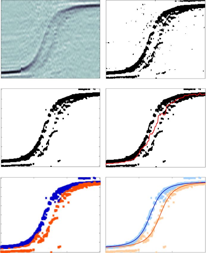
2                                         G.D. Rocha et al.: Acta Acustica 2021, 5, 18

apply to street vehicles or airplanes in very large distance.
When it comes to the simulation of dynamic scenes with
moving sound sources and moving listeners, near-field
conditions are also relevant, so that the vehicle source is
perceived as a spatially extended source. This is obvious
for trains and trams. However, for street vehicles such as
cars there is no comprehensive approach to this aspect. In
this paper, we develop a technique to extract data for
extended sound sources. This data can be used for physi-
cally-based synthesis of virtual sources in virtual acoustic
environments.
    The estimations of speed and wheelbase from acoustic
signals have been reported in the literature, with larger pre-
dominance of the former [13, 15–18] over the latter [14, 15].
In [16], for instance, a maximum likelihood approach is pro-      Figure 1. Two-microphone setup for delay s0 and direction of
posed for speed estimation, which resulted in more accurate       arrival / estimation.
and robust estimates when compared to the conventional
analysis of sequential short-time cross-correlations.                 Assuming free-field conditions, the DoA needed for
    The direction of arrival (DoA) method proposed in this        tracking the source and represented by azimuth angle /,
paper combines time difference of arrival (TDoA) estimates        might be estimated by,
of audio signals in a pair of microphones during a determined                                    cs
                                                                                                     0
observation interval. From the results presented in [19],                             / ¼ arccos       ;              ð3Þ
which compared several DoA estimation algorithms for car                                           d
pass-by recordings, it was concluded that the best TDoA           where c is the sound speed and s0 denotes the TDoA
estimates were obtained with the generalized cross-               between the two microphone signals.
correlation with phase transform (GCC-PHAT) method                   The estimator presented next was tested for DoA esti-
[20, 21]. In light of this result, in this work the GCC-PHAT      mation of vehicle sound sources in a previous work [19],
algorithm was employed with the purpose of generating             in which five algorithms were compared when executing
cross-correlation estimates of the signals simultaneously         such task. The results indicated two algorithms as suitable
acquired by the two-microphones, for different time-lags.         choices, as shown next.
A matrix containing the cross-correlation values of succes-
sive time intervals, while the car is close to the microphone     2.1 Generalized cross-correlation method
array, is formed. By applying image processing techniques
to this matrix, the time arrival differences of the predomi-          The cross correlation is a measure of similarity between
nant source signals are emphasized. Then, using a curve           two signals, which is expressed as a function of the delay s0
fitting procedure, which employs a dynamical model for             between them. For white noise signals that differ only by a
the vehicle sound signal, the directions of sound arrival from    time delay s0, the cross-correlation function presents a well-
the front and rear tires are obtained. From parameters            defined peak, with the maximum value occurring for a lag s
extracted from these curves, car speed and wheelbase esti-        equal to s0. For colored noise, such as present in tire noise,
mates can be obtained. Since information from the entire          the generalized cross-correlation method applies a normal-
pass-by time range is employed to generate such estimates,        ization function to the cross-power spectrum of the two-
they are more accurate than those based on data from short        microphone signals in order to obtain a more prominent
periods.                                                          peak in the cross-correlation function [20], making it easier
                                                                  to estimate the TDoA.
                                                                      The cross-power spectrum of the two-microphone dis-
2 Direction of arrival estimation                                 crete-time signals, x1(n) and x2(n), can be recursively esti-
                                                                  mated by [22],
    Acoustic source localization might be achieved by time-
delay estimation when more than one input channel is               S^x1x2 ðm; kÞ ¼ aS^x1x2 ðm  1; kÞ þ ð1  aÞX 1 ðm; kÞX 2 ðm; kÞ;
available. Let us consider the setup depicted in Figure 1.
A two-microphone array with inter-sensor distance d is                                                                             ð4Þ
placed parallel to a road lane. If a single source contribution
                                                                  where X1(m, k) and X2(m, k) are, respectively, the N-point
is assumed, microphone signals are modeled as,
                                                                  discrete Fourier transforms (DFT) of the windowed micro-
                     x1 ðtÞ ¼ sðtÞ þ n1 ðtÞ;               ð1Þ    phone signals w(n  mJ)x1(n) and w(n  mJ)x2(n), with m
                                                                  being the frame index and k 2 {0, . . ., N  1} the discrete
                  x2 ðtÞ ¼ sðt  s0 Þ þ n2 ðtÞ;            ð2Þ    frequency index. The N-length sequence w(n) usually
                                                                  employed in audio applications is the Hamming window
where s(t) is the source signal and n1(t), n2(t) are the noise    with shift-size J = N/2. The exponential weighting coeffi-
components.                                                       cient a is empirically set to a = 0.7.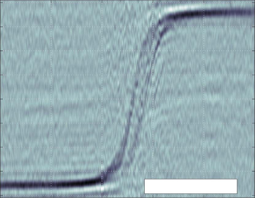
G.D. Rocha et al.: Acta Acustica 2021, 5, 18                                          3

   The generalized cross-correlation function for frame m is
then calculated as,
                             X
                             N 1 ^
                                    S x1x2 ðm; kÞ j2pN nk
           ^ x1x2 ðm; nÞ ¼ 1
           R                                    e ;     ð5Þ
                           N      S^x1x2 ðm; kÞ
                            k¼0

with n 2 {0, . . ., N  1}. The power spectrum normaliza-
tion factor employed in Equation (5) is the cross-power
estimate magnitude, resulting in a spectral function
known as phase transform (PHAT) of S^ x1x2 ðm; kÞ. The
inverse DFT of such function produces the generalized
cross-correlation function R    ^ x1x2 ðm; nÞ, which presents
sharper peaks for most audio signals and gives rise to
the GCC-PHAT method [20].
     Finally, the TDoA for frame m is estimated from
^ x1x2 ðm; nÞ as follows:
R
               s0m                       ^ x1x2 ðm; nÞ;
                    n0 ðmÞ ¼ arg max R                   ð6Þ
                T                    n                           Figure 2. TDoA estimate obtained by the GCC-PHAT
                                                                 algorithm.
where T is the sampling period of the discrete-time micro-
phone signals x1(n) and x2(n).

3 Two-axle vehicle tracking
    The TDoA estimation of Equation (6) provides a unique
value for each time window, corresponding to the sound of
the dominant source captured by the microphone signals.
Therefore, one can conclude that the GCC-PHAT algo-              Figure 3. Schematic diagram of the proposed two-source DoA
rithm, derived for a single sound source, is not suitable for    estimation system.
detecting separately the various noises produced by vehicles.
The generalized cross-correlation function of Equation (5)
                                                                     Single-source estimators in their original formulation
calculated from the signals of a car pass-by acquired by a
two-microphone horizontal array is shown in Figure 2,            provide a single DoA estimated curve as output, formed
where the darker the gray level, the higher the generalized      by the maximum value estimations for the various time
cross-correlation value. The GCC-PHAT estimates,                 frames. Such single-source estimate stage is ignored in the
obtained from the dominant GCC peaks by Equation (6),            proposed system and is replaced by the processing which
are shown by the blue curve. It can be observed that when        accounts for two sources. The matrix A(t, s) is used as an
the car passes in front of the microphone array, the esti-       input data for the image processing stage, which handles
mated TDoA alternates between the directions of the front        the information of all relevant time frames together. This
and rear vehicle axles.                                          is possible for offline applications such as the one aimed in
                                                                 this project.
    To overcome this problem, we propose the two-source
                                                                     Besides the data from the single-source TDoA estimator,
DoA estimation system depicted in Figure 3, where image
                                                                 the curve fitting algorithm must be fed with a curve model.
processing techniques followed by a curve fitting method
are appended to the single-source GCC-PHAT algorithm.            A rough model for TDoA curves is derived in agreement to
Although GCC-PHAT is used throughout this work, the              pass-by dynamic and geometric characteristics, as shown in
system was developed to allow changing and testing differ-       Section 3.1. Moreover, the steps comprised in the “Two-
ent single source TDoA estimators, such as those examined        source Extension” block are explained in Sections 3.2 and
in [19]. Optional algorithms, such as maximum-variance           3.3. Data pre-processing stage aims at cleaning and adjust-
distortionless response (MVDR) [23, 24] and least-mean           ing input matrix A(t, s) by removing spurious and irrelevant
square (LMS) [25, 26] algorithms, can obtain the TDoA            data. This is carried out in order to improve the curve fitting
estimations using different criteria, but they must have         performance.
essential characteristics that are exploited in our system.
All single-source estimation algorithms must use two-chan-       3.1 Theoretical TDoA model
nel audio recordings and provide as output a matrix A(t, s),
which is a function of the time index t and of the possible         The theoretical evolution of TDoA over time is obtained
discrete time delays s between the microphone signals. In        by calculating the difference in sound path between the
GCC-PHAT algorithm, this matrix corresponds to auto-             source and the two microphones separated by a distance d.
correlation matrix estimate R  ^ x1x2 ðm; nÞ, since the delays      In the following derivation, it is assumed that: the
are obtained from Equation (6).                                  source is at ground level, in the z = 0 plane; the microphone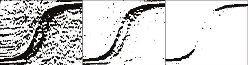
4 G.D. Rocha et al.: Acta Acustica 2021, 5, 18
array is in the y = 0 plane, with its axis parallel to the z = 0 0.8
plane and at the height h, measured from the floor up to the
0.6
array center; the vehicle velocity v is parallel to the x-axis
and has constant magnitude vx.1 From simple trigonometric 0.4
relations and assuming that the vehicle speed is much
(ms)
smaller than the sound speed, it can be demonstrated that 0.2
the time difference of arrival of the source sound in the two 0
sensors in a given snapshot t is given by,
Delay
-0.2
l2 ðtÞ l1 ðtÞ
s ; ð7Þ -0.4
vx
-0.6
where,
2 -0.8
l21 ðtÞ ¼ h2 þ s2y þ ðsx ðtÞ d=2Þ ; ð8Þ 0 0.5 1 1.5 2 2.5 3
Time (s)
2
l22 ðtÞ ¼ h2 þ s2y þ ðsx ðtÞ þ d=2Þ ; ð9Þ
Figure 4. Theoretical TDoA curve for a 60 km/h moving
vehicle.
with sx and sy equal to the distances between the source
and the x = 0 and y = 0 planes, respectively.
An illustration of the theoretical TDoA behavior for
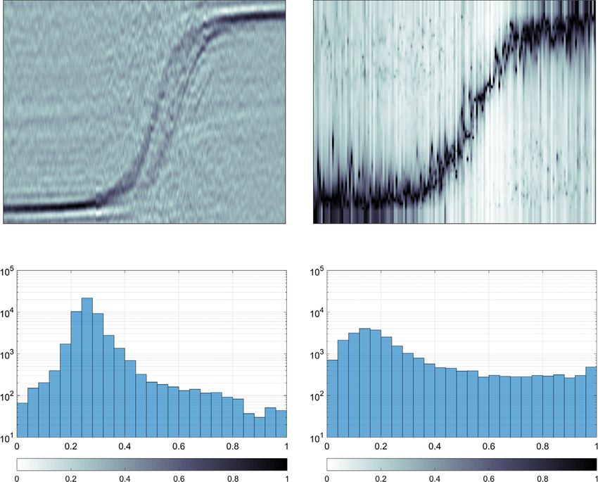
the performance of the curve fit method. For this reason,
constant speed is shown in Figure 4, where s was obtained
the input data is appropriately filtered, in an attempt to
from Equations (7)–(9) with vx = 60, sy = 3, d = 0.25, and,
reduce noise.
sx ðtÞ ¼ ðt t0 Þvx ; ð10Þ First, the grayscale image is converted into a binary
image using a threshold value, selected based on empirical
where t0 = 1.5 s is the time instant in which the vehicle tests. A binary image, composed of either zero or one val-
passes exactly in front of the microphone array. ues, is required by signal processing algorithms to perform
morphological operations, such as dilation and erosion.
3.2 Data pre-processing Such operations are used to reduce noise and to provide
more precise edge detection to fit the DoA estimation. This
The data provided by the single-source DoA estimation empirical optimization leads to different threshold values
algorithm goes through a pre-processing stage consisting of for the alternative single-source DoA estimators, as a conse-
level scaling and noise reduction to adjust it to the curve quence of the diversity in the pixel distribution of the
fitting algorithm. Using the GCC-PHAT, the matrix generated images. To illustrate this effect, the images gen-
A(t, s) contains the generalized cross-correlation between erated by GCC-PHAT and MVDR are shown in Figure 5,
the two-microphone signals for different time windows together with the respective histogram plots. The histogram
and lag values. Alternative DoA estimation algorithms graphs indicate how pixel gray-levels are distributed across
can provide metrics other than the cross-correlation. The intensity levels. While for GCC-PHAT pixels are highly
scaling of the input data is, therefore, needed in order to concentrated around the 0.3 level, for the MVDR they
adjust the two-dimensional data contained in A(t, s), so are more evenly distributed across the different levels. This
that it can be treated as a digital image representation, with clear difference between images indicates the relevance of
values in the grayscale range. This image will be further choosing an appropriate threshold value. Binary images
processed to reduce noise by two-dimensional filters. generated for different thresholds are depicted in Figure 6.
Due to the decreasing amplitude of the sound propagat- A trade-off between removing noise and maintaining suffi-
ing over long distances between the source and the micro- cient relevant data is observed.
phones, the relevant audio data is concentrated around Next, we describe the image processing approach pro-
t = t0, when source-receiver distance is minimum and posed for noise reduction, with the illustrative results of
signal-to-noise ratio is maximum. Thus, the data scaling the main steps shown in Figure 7. The morphological open-
is followed by cropping, which aims to discard irrelevant ing operation (dilatation followed by erosion [27, 28]) is per-
audio recordings, acquired when the vehicle is far away formed on the binary image using a square structuring
from the microphones. A 3-length data window is selected element, which eliminates isolated black pixels. Most noise
around the sample corresponding to maximum signal power is removed after the opening operation, as can be observed
(t = t0) and the rest is ignored. in Figure 7c.
In a real pass-by scenario, the interfering noise generated In this image, two main parallel curves are highlighted,
by other sources, instead of the vehicle, can corrupt the indicating the presence of two dominant noise sources.
recordings. Depending on noise source position, intensity The time shift between them is in accordance with the
and spectral content, this interference can seriously impair sounds emitted by sources whose distance is the average
1
Similar TDoA derivation can be performed for other config- wheelbase in passenger cars. Therefore, it can be concluded
urations. that these sound components resulted from the noiseG.D. Rocha et al.: Acta Acustica 2021, 5, 18 5
Figure 5. Images obtained with (a) GCC-PHAT and (b) MVDR single-source estimators, with respective pixel histograms in
(c) and (d).
Figure 6. Binary images after applying the following threshold values: (a) 0.025, (b) 0.1 and (c) 0.25.
generated by the vehicle’s front and rear axles. This assump- non-zero values of each column of the binary image. Then,
tion is supported by the work presented in [14], in which a this curve is used as the border line to separate the data into
pair of loudspeakers was placed in front of the vehicle’s two sets. The data to the left of the average curve, repre-
wheels and the resulting TDoA estimate exhibits the same sented in blue in Figure 7e, is associated with the emission
pattern observed in Figure 7a. of the front-axle tires (since the left curve appears ahead
In order to track the noise emitted by the tires of in time). Likewise, the data to the right of the average
each axle separately, two distinct data sets must be pro- curve, displayed in orange in Figure 7e, is associated with
vided to the curve fitting algorithm. Firstly, an “average the emission of the rear-axle tires. These two data sets,
curve” is calculated to define the points which belong to corresponding to the left and right pixels with respect to
each axle. This curve is represented by the red line in the average TDoA curve, respectively, are delivered to
Figure 7d and is obtained by averaging the indexes of the the curve fitting stage.6 G.D. Rocha et al.: Acta Acustica 2021, 5, 18
0.8
0.6
0.4
(ms)
0.2
0
Delay
-0.2
-0.4
-0.6
-0.8
0.8
0.6
0.4
(ms)
0.2
0
Delay
-0.2
-0.4
-0.6
-0.8
0.8
0.6
0.4
(ms)
0.2
0
Delay
-0.2
-0.4
-0.6
-0.8
0 1 2 3 0 1 2 3
Time (s) Time (s)
Figure 7. Illustration of pre-processing and curve fitting results. (a) Gray-scale image; (b) binary image; (c) image after
morphological opening; (d) mean TDoA curve; (e) selected data; (f) fitted curves.
3.3 Curve fitting method The cost function is weighted iteratively using bisquare
weights [33, 34].
The theoretical model obtained for the TDoA in The curve parameters are initialized with random
Equation (7) serves here as prototype to fit the data, and values from a Gaussian distribution. The unknown vari-
the least-squares algorithm is used as optimizer. In light of ables in Equation (7) are the instant t0, distance sy and
the non-linear theoretical TDoA graph in Figure 4, the curve the speed vx. For each of them, we can define lower and
fitting method is applied to the image resulting from the upper limits. These intervals can be used as prior knowledge
pre-processing stage using a trust region for non-linear for initialization by setting the mean values of the random
optimization [29–32]. In addition, spurious data may not distributions as the centers of the defined intervals. The
be eliminated in pre-processing and may appear as anomaly result is a fitted curve for each data vector, as shown in
in the selected data. This is especially problematic, given the Figure 7f.
known sensitivity of least-squares algorithms to outliers. In The fitting algorithm finds the model parameter values
this sense, a robust least squares approach is employed. that minimize the mean squared error between data pointsG.D. Rocha et al.: Acta Acustica 2021, 5, 18 7
Table 1. Vehicles used in pass-by tests.
Vehicle ID Car model Transmission
1 Volkswagen Gol 1.0 Manual
2 Jeep Renegade 1.8 Automatic
3 Mitsubishi ASX 2.0 Automatic
4 Hyundai Creta 1.6 Automatic
70
60
Figure 8. 3D representation of the measurement setup: micro-
phone array parallel to the vehicle trajectory; height h from the 50
Speed (km/h)
floor up to the array center; distance l between the source and
40
the reference sensor.
30
and the corresponding fitted curve values. The speed is a 20
parameter of the model of Equation (7) and is estimated
10
directly in the optimization process. The two curves are Estimate Real
adjusted independently and the estimated parameters, 0
1 2 3 4 5 6 7 8 9 10 11 12 13 14 15 16 17 18 19 20 21 22 23
including speed, may be slightly different for each axle.
Test ID
For simplicity, the average value is used as speed estimate.
On the other hand, the wheelbase is estimated as the dis- Figure 9. Speed estimates obtained using the proposed system
tance between the fitted curves. This distance is evaluated with random parameter initialization.
when the delay s = 0, that is, when each axle is symmetri-
cally in front of the microphone array. In a controlled test
scenario, the optimized parameters can be compared to the On the other hand, if only the experiments with measured
actual values as a measure of the accuracy of the algorithm. speed above 50 km/h are considered, the average absolute
error increases to 18.1 km/h.
A tendency of underestimating the car velocity is
4 Experimental results observed in Figure 9, especially for speeds above 50 km/h.
One possible cause could be the simplistic model used for
A set of experiments was conducted with signals the theoretical evolution of the TDoA over time, which
acquired by an array of two microphones, aligned horizon- assumed constant speed much smaller than the speed of
tally and spaced by d = 0.25 m. It consisted of cars passing sound and did not take into account the Doppler effect.
on front of the array, one at a time, in a quiet region, with- The curves obtained for Test 22, which presented the
out traffic and with negligible background noise, located at largest speed error, are shown in blue in Figure 10. Despite
the Brazilian National Institute of Metrology (INMETRO), the poor speed estimation result, the fitted curves are well
Rio de Janeiro, Brazil. Four different passenger cars were adjusted to the delays obtained for the noise of the two
used in the experiments, as detailed in Table 1. Each car axles of the vehicle, indicating that the error is not caused
passed by the microphone array at constant speeds of by the fitting optimization process, but by the theoretical
around 30, 50, 60 and 70 km/h and with a distance model of the curve.
sx = 2.0 ± 0.2 m from the array origin, as depicted in The wheelbase estimation results are presented in
Figure 8. A GPS device placed inside the vehicle was used Figure 11 for the experiments in ascending speed order.
to estimate the speed, based on the car position and time. Blue circles and red stars indicate estimated and measured
The vehicle wheelbases were obtained from information values, respectively. The average estimation error was
provided by their respective manufacturers. 26 cm. Unlike speed estimation, wheelbase results do not
The performance of the proposed system was evaluated appear to be correlated to the vehicle speed. This is in
by comparing the actual values of the speed and wheelbase agreement with the sensitivity study carried out in [13],
of the vehicles, measured during the experiments, with the where the increase of vehicle speed had no influence in
estimated ones. The speed estimates are represented by blue wheelbase estimation, but caused larger mean error and
circles in Figure 9 for each test, while measured values are standard deviation in speed estimation.
represented by red stars. Test results were sorted in ascend- Tests 3 and 8 stand out in Figure 11 for presenting high
ing order of the measured speed values for visualization pur- errors. These two tests share similarities which explain
poses. The average absolute error was 10.8 km/h. It can be the obtained result. The audio files used in Tests 3 and 8
seen in this figure that the estimation error clearly increases contain sound emissions from the same vehicle, identified
for higher speeds, especially for values above 50 km/h. If as Car 2 in Table 1. Car 2 emissions were also registered
only the experiments with measured speed below 50 km/h in Tests 4, 15, 16, 19 and 22, which resulted in estimation
are considered, the average absolute error is 6.3 km/h. errors below 30 cm. However, for pass-by trials 3 and 8,8 G.D. Rocha et al.: Acta Acustica 2021, 5, 18
4
0.8
3.5
0.6
Wheelbase (m)
0.4 3
(ms)
0.2 2.5
0
2
Delay
-0.2
1.5
-0.4 GCC Real
1
-0.6 1 2 3 4
Estimated TDoA Vehicle ID
-0.8
0 1 2 3 4 5 Figure 12. Average wheelbase estimate for each vehicle.
Time (s)
Figure 10. Tracking results for the highest-speed-error test. 70
60
4
50
Speed (km/h)
40
3
Wheelbase (m)
30
20
2
10
Estimate Real
0
1
1 2 3 4 5 6 7 8 9 10 11 12 13 14 15 16 17 18 19 20 21 22 23
Test ID
GCC Real
0 Figure 13. Speed estimates obtained using the proposed
1 2 3 4 5 6 7 8 9 10 11 12 13 14 15 16 17 18 19 20 21 22 23
system and parameter initialization with measured speed values.
Test ID
Figure 11. Wheelbase estimates obtained using the proposed 4
system with random parameter initialization. Errors of Test IDs
3 and 8 are due to the loud engine noise of Car 2, which was
forced to not change gears during the passage. 3
Wheelbase (m)
the vehicle was forced to travel in low gear and high engine
2
speed. Engine noise is affected by engine speed [4] and could
increase to a level comparable to or higher than tire noise.
The proposed system assumes that the tire noise is the 1
dominant sound source and, when this condition is not
maintained, such as in Tests 3 and 8, it is expected that GCC Real
the estimation of delay and wheelbase will fail. 0
1 2 3 4 5 6 7 8 9 10 11 12 13 14 15 16 17 18 19 20 21 22 23
Given that the same four vehicles were used throughout
Test ID
the 23 experiments, an average wheelbase estimate is calcu-
lated and depicted in Figure 12. For each vehicle, blue circle Figure 14. Wheelbase estimates obtained using the proposed
indicates the wheelbase estimate averaged over all trials in system and parameter initialization with measured speed values.
which the vehicle was recorded and red star indicates the
measured value. Vehicle 2 presented the highest wheelbase
estimation error, equal to 32 cm, due to increased engine this scenario is 4.9 km/h. The underestimate tendency is
noise, whereas Cars 1, 3 and 4 presented errors of 14, 24 even more noticeable, as it happens for 22 (or 95%) of the
and 12 cm, respectively. 23 tests. The increasing error for higher speeds is still
A second set of estimations is performed using measured present, although the absolute error for speeds above
speed values to initialize the parameters, instead of random 50 km/h decreased to 7.4 km/h.
initialization. As expected, speed estimation error decreases, In contrast, wheelbase estimation is barely affected by
as depicted in Figure 13, and the average absolute error in this change in initialization. The estimates in Figure 14G.D. Rocha et al.: Acta Acustica 2021, 5, 18 9
are almost identical to the ones in Figure 11 and the same to the National Institute of Metrology, Standardization
26 cm average error was obtained. The wheelbase is esti- and Industrial Quality (INMETRO), in the figures of
mated as the distance between both fitted curves when Paulo M. Massarani and Zemar M. D. Soares for record-
s = 0. Therefore, this value is highly correlated to parame- ings assistance and to prof. Fernando A. N. C. Pinto, from
ter t0, which indicates the instant when the curve crosses Laboratory of Acoustics and Vibration from COPPE/
s = 0. Speed parameter, in contrast, affects the curve slope UFRJ, for instrumentation support.
around t0 and for that reason does not present an impact on
wheelbase estimates.
Conflict of interest
5 Conclusion Author declared no conflict of interests.
In this paper, we presented a method for separately
tracking the axles of a two-axle vehicle using a pair of References
microphones. The approach is divided in two main steps:
1. M. Vorländer: Auralization: Fundamentals of Acoustics,
first, a time difference of arrival estimator calculates Modelling, Simulation, Algorithms and Acoustic Virtual
short-time cross-correlations between the microphone Reality, 2nd ed. Springer Nature, 2020.
signals over an observation time interval, which are pre- 2. B. Masiero, W.D. Fonseca, M. Müller-Trapet, P. Dietrich,
processed and stored in a data matrix. Secondly, the matrix Auralization of pass-by beamforming measurements, in EAA
with the accumulated treated data is used to obtain two EUROREGIO, 15–18 September 2010, Ljubljana, Slovenia.
curves, corresponding to the direction of the tire noise of 2010.
the two axles. From the curve fitting results, the speed 3. M. Nilsson, J. Forssén, P. Lundén, A. Peplow, B. Hellström:
Listen Auralization of Urban Soundscapes. Stockholm
and wheelbase of the vehicle are estimated. This modular- University, Chalmers University of Technology, Sonic
ized approach allows easier testing new algorithms and Studio, KTH Royal Institute of Technology, University
models and comparing their performance. College of Arts, Crafts and Design, 2011.
In the pre-processing stage, the concatenated cross- 4. R. Pieren, T. Bütler, K. Heutschi: Auralization of accelerat-
correlation data is processed altogether using image pro- ing passenger cars using spectral modeling synthesis. Applied
cessing techniques. Thresholding and opening operations Sciences 6, 1 (2016) 5.
5. L. Jiang, M. Masullo, L. Maffei, F. Meng, M. Vorländer: A
are applied to the image for noise reduction. The choice
demonstrator tool of web-based virtual reality for participa-
of the threshold value is critical for the overall system per- tory evaluation of urban sound environment. Landscape and
formance and should be further investigated and optimized. Urban Planning 170 (2018) 276–282.
Image pixels are then separated into two data vectors, 6. P.H.T. Zannin, F.B. Diniz, W.A. Barbosa: Environmental
which are separately used in the two-curve fitting model. noise pollution in the city of Curitiba, Brazil. Applied
The proposed system relies on a theoretical model for the Acoustics 63, 4 (2002) 351–358.
time difference of arrival which should be improved in 7. P.H. Zannin, A. Calixto, F.B. Diniz, J.A. Ferreira: A survey
of urban noise annoyance in a large Brazilian city: The
further studies. importance of a subjective analysis in conjunction with an
The results for vehicle noise tracking were satisfactory objective analysis. Environmental Impact Assessment
and can be applied, as intended, for obtaining source models Review 23, 2 (2003) 245–255.
to be used in acoustic virtual reality systems. The speed 8. B. Jakovljevic, K. Paunovic, G. Belojevic: Road-traffic noise
estimate is not accurate, especially at high speeds, with and factors influencing noise annoyance in an urban popu-
the absolute mean speed estimate calculated only over lation. Environment International 35, 3 (2009) 552–556.
low speed experiments equal to 6.3 km/h and calculated 9. S. Agarwal, B.L. Swami: Road traffic noise, annoyance and
community health survey – a case study for an Indian city.
over all experiments equal to 18.1 km/h. In contrast, the Noise and Health 13, 53 (2011) 272–276. https://doi.org/
wheelbase estimation errors were not correlated to the 10.4103/1463-1741.82959.
speed estimation errors, with average absolute error equal 10. K. Heutschi, E. Bühlmann, J. Oertli: Options for reducing
to 26 cm. With this, we can continue to build improved noise from roads and railway lines. Transportation Research
models of virtual vehicles as sources in virtual acoustic Part A: Policy and Practice 94 (2016) 308–322.
environments. 11. U. Sandberg: Tyre/road Noise: Myths and Realities. Statens
väg-och transportforskningsinstitut, 2001.
It is planned to apply the technique in long-term
12. D. O’Boy, A. Dowling: Tyre/road interaction noise –
measurements at busy roads. With additional methods to numerical noise prediction of a patterned tyre on a rough
identify categories of vehicle types and their speeds by video road surface. Journal of Sound and Vibration 323, 1–2 (2009)
annotation, the aim is to fill a database of parametric data 270–291.
of street vehicles. 13. P. Marmaroli, J.-M. Odobez, X. Falourd, H. Lissek: A
bimodal sound source model for vehicle tracking in traffic
monitoring, in 2011 19th European Signal Processing Con-
ference, IEEE. 2011, pp. 1327–1331.
Acknowledgments 14. P. Marmaroli, M. Carmona, J.-M. Odobez, X. Falourd, H.
Lissek: Observation of vehicle axles through pass-by noise:
The authors would like to thank CAPES and DAAD A strategy of microphone array design. IEEE Transactions on
for partially supporting this research. We are also grateful Intelligent Transportation Systems 14, 4 (2013) 1654–1664.10 G.D. Rocha et al.: Acta Acustica 2021, 5, 18
15. V. Cevher, R. Chellappa, J.H. McClellan: Vehicle speed 25. F. Reed, P. Feintuch, N. Bershad: Time delay estimation
estimation using acoustic wave patterns. IEEE Transactions using the lms adaptive filter–static behavior. IEEE Transac-
on Signal Processing 57, 1 (2008) 30–47. tions on Acoustics, Speech, and Signal Processing 29, 3
16. R. López-Valcarce, C. Mosquera, F. Pérez-González: Esti- (1981) 561–571.
mation of road vehicle speed using two omnidirectional 26. E. Ferrara: Fast implementations of lms adaptive filters.
microphones: A maximum likelihood approach. EURASIP IEEE Transactions on Acoustics, Speech, and Signal Pro-
Journal on Advances in Signal Processing 2004, 8 (2004) cessing 28, 4 (1980) 474–475.
929146. 27. R.M. Haralick, L.G. Shapiro: Computer and Robot Vision,
17. P. Borkar, L.G. Malik: Review on vehicular speed, density Vol. 1. Addison-Wesley Reading, 1992.
estimation and classification using acoustic signal. Interna- 28. R.M. Haralick, S.R. Sternberg, X. Zhuang: Image analysis
tional Journal for Traffic & Transport Engineering 3, 3 using mathematical morphology, in IEEE Transactions on
(2013) 331–343. Pattern Analysis and Machine Intelligence, no. 4, IEEE.
18. F. Peréz-González, R. López-Valcarce, C. Mosquera: Road 1987, pp. 532–550.
vehicle speed estimation from a two-microphone array, in 29. J.J. Moré, D.C. Sorensen: Computing a trust region step.
2002 IEEE International Conference on Acoustics, Speech, SIAM Journal on Scientific and Statistical Computing 4, 3
and Signal Processing, Vol. 2, IEEE. 2002, p. II–1321. (1983) 553–572.
19. G.D. Rocha, F.R. Petraglia, J.C.B. Torres, M.R. Petraglia: 30. M.A. Branch, T.F. Coleman, Y. Li: A subspace, interior, and
Direction of arrival estimation of acoustic vehicular sources, conjugate gradient method for large-scale bound-constrained
in Proceedings of the 23rd International Congress on minimization problems. SIAM Journal on Scientific Com-
Acoustics, 9–13 September, Aachen, Germany. 2019. puting 21, 1 (1999) 1–23.
20. C. Knapp, G. Carter: The generalized correlation method for 31. R.H. Byrd, R.B. Schnabel, G.A. Shultz: Approximate
estimation of time delay. IEEE Transactions on Acoustics, solution of the trust region problem by minimization over
Speech, and Signal Processing 24, 4 (1976) 320–327. two-dimensional subspaces. Mathematical Programming 40,
21. D. Hertz, M. Azaria: Time delay estimation between two 1–3 (1988) 247–263.
phase shifted signals via generalized cross-correlation meth- 32. T.F. Coleman, Y. Li: An interior trust region approach for
ods. Signal Processing 8, 2 (1985) 235–257. nonlinear minimization subject to bounds. SIAM Journal on
22. G. Doblinger: Localization and tracking of acoustical sources, Optimization 6, 2 (1996) 418–445.
in Topics in Acoustic Echo and Noise Control, Springer. 33. P.W. Holland, R.E. Welsch: Robust regression using
2006, pp. 91–122. iteratively reweighted least-squares. Communications in
23. S. Vorobyov: Principles of minimum variance robust adap- Statistics-Theory and Methods 6, 9 (1977) 813–827.
tive beamforming design. Signal Processing 93, 1 (2013) 34. J.O. Street, R.J. Carroll, D. Ruppert: A note on computing
3264–3277. robust regression estimates via iteratively reweighted least
24. J. Capon: High-resolution frequency-wavenumber spectrum squares. The American Statistician 42, 2 (1988) 152–154.
analysis. Proceedings of the IEEE 57, 8 (1969) 1408–1418.
Cite this article as: Rocha GD, Torres JCB, Petraglia MR & Vorländer M. 2021. Direction of arrival estimation of partial sound
sources of vehicles with a two-microphone array. Acta Acustica, 5, 18.You can also read