Early Detection of Defects through the Identification of Distortion Characteristics in Ultrasonic Responses - MDPI
←
→
Page content transcription
If your browser does not render page correctly, please read the page content below
mathematics

Article
Early Detection of Defects through the Identification of
Distortion Characteristics in Ultrasonic Responses
Pietro Burrascano *                and Matteo Ciuffetti

                                          Dipartimento di Ingegneria, Università di Perugia, 06125 Perugia, Italy; matteo.ciuffetti@studenti.unipg.it
                                          * Correspondence: pietro.burrascano@unipg.it

                                          Abstract: Ultrasonic techniques are widely used for the detection of defects in solid structures. They
                                          are mainly based on estimating the impulse response of the system and most often refer to linear
                                          models. High-stress conditions of the structures may reveal non-linear aspects of their behavior
                                          caused by even small defects due to ageing or previous severe loading: consequently, models suitable
                                          to identify the existence of a non-linear input-output characteristic of the system allow to improve
                                          the sensitivity of the detection procedure, making it possible to observe the onset of fatigue-induced
                                          cracks and/or defects by highlighting the early stages of their formation. This paper starts from an
                                          analysis of the characteristics of a damage index that has proved effective for the early detection of
                                          defects based on their non-linear behavior: it is based on the Hammerstein model of the non-linear
                                          physical system. The availability of this mathematical model makes it possible to derive from it a
                                          number of different global parameters, all of which are suitable for highlighting the onset of defects
                                          in the structure under examination, but whose characteristics can be very different from each other.
                                          In this work, an original damage index based on the same Hammerstein model is proposed. We
                                          report the results of several experiments showing that our proposed damage index has a much higher

                                   sensitivity even for small defects. Moreover, extensive tests conducted in the presence of different
                                          levels of additive noise show that the new proposed estimator adds to this sensitivity feature a better
Citation: Burrascano, P.; Ciuffetti, M.
                                          estimation stability in the presence of additive noise.
Early Detection of Defects through
the Identification of Distortion
Characteristics in Ultrasonic             Keywords: non-destructive evaluation; pulse compression; non-linear systems; Hammerstein model
Responses. Mathematics 2021, 9, 850.
https://doi.org/10.3390/math9080850

Academic Editor: Mario Versaci            1. Introduction
                                               The use of techniques to detect non-linear behaviors in systems, aimed at early stage
Received: 8 March 2021                    detection and identification of defects in structures and materials, is a rapidly evolving
Accepted: 12 April 2021
                                          research field with great potential for application in industrial production and in peri-
Published: 13 April 2021
                                          odic tests aimed at safety and durability. Increasingly sophisticated techniques are being
                                          consolidated for the early detection of imperfections, defects, and micro-fractures due to
Publisher’s Note: MDPI stays neutral
                                          oxidation or resulting from the fatigue behavior of materials [1–3]. The usual ultrasonic
with regard to jurisdictional claims in
                                          techniques can detect flaws of the order of wavelength. To detect defects of smaller size
published maps and institutional affil-
                                          using ultrasonic excitations of the same frequency, particular phenomena that induce
iations.
                                          non-linear behavior in the response must be considered, and this allows the detection of
                                          the much smaller flaws.
                                               Non-destructive techniques for defect detection can be divided into linear and non-
                                          linear. Taking ultrasonic techniques as a reference, linear methods are based on the esti-
Copyright: © 2021 by the authors.         mation of parameters such as attenuation, transmission, and reflection coefficients, thus
Licensee MDPI, Basel, Switzerland.
                                          implicitly likening the analyzed system to a linear one whose impulse response is measured.
This article is an open access article
                                          Based directly on propagation phenomena, these techniques are capable of detecting, in
distributed under the terms and
                                          the material, discontinuities of a size comparable to the wavelengths involved: this makes
conditions of the Creative Commons
                                          these techniques unsuitable for detecting extremely small fractures, if smaller than this size;
Attribution (CC BY) license (https://
                                          increasing the frequency of the signal used may allow the detection of defects of propor-
creativecommons.org/licenses/by/
4.0/).
                                          tionally smaller size, but is faced with limitations in the availability of suitable transducers

Mathematics 2021, 9, 850. https://doi.org/10.3390/math9080850                                             https://www.mdpi.com/journal/mathematics
Mathematics 2021, 9, 850 2 of 14
and significant increases in propagation attenuation. The non-linear techniques have the
potential to overcome, within certain limits, the wavelength constraint, as they aim at
detecting how the waveform of the signal injected into the system changes due to the intro-
duction of further harmonic components in the response of the non-linear system, which
can make the signal waveform significantly different from that of the excitation signal.
The mechanism behind the formation of non-linear components in the response can
be interpreted in a very simple way by considering the interaction between the crack facing
surfaces when they are hit by the ultrasonic wave propagating through the medium: in the
phase in which the propagating wave generates compression, a contact is created between
the two faces of the crack, and this contact causes the propagation of the ultrasonic wave
to occur in an unattenuated manner; in the semi-period in which the propagating wave,
instead, generates tension in the medium, the two walls detach and the propagation occurs
in a strongly different manner, such that the tension half-waves are significantly more
attenuated. The mechanism that makes the behavior of the compression and tension phases
different during each period is such as to produce a non-linear distortion of the propagating
signal, which generates additional harmonic components in the response of the system,
and this occurs even if the transverse dimensions of the crack are small compared to the
wavelength of the propagating signal [4,5].
A number of defect detection techniques based on non-linear behavior can be de-
fined according to the particular aspect that is considered, among the features resulting
from the non-linear characteristic of the examined system; one can distinguish between
methods that detect the presence of higher order harmonics [6–8], methods that analyze
the frequency shift of resonances [9,10], vibro-acoustic modulation methods [5,11], and
frequency mixing methods, which highlight the production of non-linear combinations
of harmonic components that have been generated due to different phenomena or propa-
gation modes [12,13]. In the first case, the response is analyzed to detect the presence of
higher order harmonics: e.g., in [6], it is shown how non-linearity due to the presence of
damages manifests itself as sideband components in the spectrum of the received signal,
while in [8], a technique based on pulse compression and the scalar subtraction method
are compared under the same experimental conditions to highlight their respective sen-
sitivities: a laboratory test experiment on mortar samples is performed to compare their
ability to detect spectral components due to early damage in samples showing a non-linear
response. To give a quantitative idea of the improvement that can be achieved in terms of
resolution by considering non-linear phenomena, we report that in [8], the experimental
results carried out on concrete bar adopting a swept sine signal, whose center frequency
is 55 kHz, allowed the detection of an U-shaped notch in the middle of the bar, whose
dimension in the direction of propagation is approximately λ/12, i.e., allowing a range res-
olution at least 3 or 4 times higher than that of the usual ultrasound techniques. Nonlinear
resonance acoustic spectroscopy studies nonlinear phenomena by analyzing the resonance
modes of a material. Granular and micro-fractured materials always show a non-linear
attenuation of the modulus of elasticity, even at very low strain levels. As a result, their
resonance frequency shifts, harmonics are generated, and amplitude-dependent damping
characteristics are observed. In undamaged materials, these phenomena are very weak.
In damaged materials, they are considerably more pronounced. In [11], it is shown that
non-fully bonded interfaces exhibit highly non-linear behavior: one of the consequences
of such non-linear behavior is the modulation of a high-frequency ultrasonic wave by a
low-frequency vibration. The vibration varies the contact area by modulating the phase
and amplitude of the higher frequency test wave passing through the damaged interface.
In [13], the authors consider the non-linear interaction of counter-propagating Lamb waves
and the resulting resonance phenomenon, and analyze the resulting overall signal in the
time domain in order to make a precise localization of the damage in the structure.
In our case, we will mainly refer to techniques that analyze higher order harmonics.
These techniques have led to extremely interesting application results: for example, [14]
explores the possible use of non-linear ultrasonic techniques, and in particular, the inter-Mathematics 2021, 9, 850 3 of 14
modulation components, for detecting the cracking due to corrosion of steel reinforcements
in concrete; in [15], a non-linear technique based on second-order harmonics is adopted to
characterize the damage present in granite samples subjected to compressive loads, and it
is shown that the non-linear parameter used is significantly more sensitive to the presence
of damage than parameters based on linear techniques.
In the present paper, we show how a well-established technique for the identification
of the non-linear Hammerstein model of the structure under investigation allows to define
a new reliable damage indicator for an early detection of possible flaws, based directly on
the parameters of the identified model. The validation of the procedure on a consolidated
integral model of the physical structure allows to compare the reliability of the proposed
method with that of a different damage indicator, proposed in the technical literature.
The comparison is also performed in the presence of high levels of additive noise: even
under these conditions, the innovative estimator we propose shows a higher sensitivity to
small-sized defects and a higher stability in the estimated value.
The paper is organized as follows: in Section 2, the theoretical aspects of the procedure
are described: Section 2.1 provides a description of the technique for the identification
of non-linear systems based on the Hammerstein model. The identification technique
adopted in this paper is based on (i) the use of a swept sine exponential signal as a pilot
input to the nonlinear system and on (ii) the processing of the corresponding response by
means of a pulse compression technique: the latter is described in Section 2.2; in the same
Section 2.2, it is also highlighted how this technique is associated with an improvement
of the signal-to-noise ratio (SNR) at the output of the matched filter. Section 2.3 then
describes the damage indicators and the simulation system adopted for the subsequent
experiments, and in particular, Section 2.3.1. describes the damage indicator proposed
in the technical literature, and Section 2.3.2. defines the original harmonic index damage
indicator that we propose in this paper. Section 2.3.3. describes the model adopted to
generate the data considered to simulate the non-linear system that was adopted for the
subsequent simulation experiments, an integral model known in the technical literature.
Section 3 describes the experimental tests performed using the proposed new estimator, the
results of which are compared with those of the other estimator considered, on synthetic
experiments; the results obtained by using the two damage indicators are discussed and
compared. In Section 4, some conclusions are drawn and the possible evolution of the
research work is indicated.
2. Modeling Non-Linearity for Damage Detection
In principle, one of the simplest methods of assessing the non-linearity characteristics
of a structure or material would be to measure the magnitude of the harmonics present
in the system’s response to a single sinusoidal excitation tone. This technique is difficult
to apply in practice, except for systems operating in a frequency range close to DC. This
is because the harmonic components quickly reach frequencies that are either outside the
operating range of the system, or outside the measurable frequency range of the sensors
used. This problem can be overcome by using different input signals, such as a couple of
sinusoidal tones: this input produces, at the output of the non-linear system, harmonic
components at frequencies which are linear combinations with integer coefficients of the
tones at the input. Among these components, we can choose an intermodulation frequency
close to the useful band of the system. The amplitude of this component allows to define
other types of estimators of the degree of non-linearity in the behavior of the system. The
amount of distortion, and therefore the amount of harmonic intermodulation components
associated with the input signal, depends on the measuring modes and increases as the
excitation signal level increases. For these reasons, the procedures for its measurement are
codified in international standards [16].
These techniques, however, are based on the frequency analysis of the signal produced
at the output of the system. They have undoubted advantages linked to their simplicity
and are computationally efficient, but they involve all the limitations of spectral analysis,Mathematics 2021, 9, 850 4 of 14
whether they refer to parametric methods based on the Fourier transform of the autocor-
relation estimate (Blackman and Tukey) or are based on the direct application of the Fast
Fourier Transform to the data (periodogram). These methods, due to the strong presence of
sidelobes associated with them, imply the impossibility of detecting harmonic components
of limited amplitude [17]. This can be a major disadvantage if we are interested in the
early detection of the onset of non-linear effects and to the first occurrence of additional
harmonic components related to such phenomena. The use of appropriate windows can
only partially limit these effects.
Alternatives have been proposed to the frequency methods, as for instance, those
based on a comparison of the input and output signals in the time domain, as is done for
example with the scaling subtraction method (SSM) technique: it extracts the non-linear
characteristic of the output waveform relying on the breaking of the superposition principle
that is induced by the elastic non-linearity of the system considered [7,8].
In our case, we focus on methods based on spectral analysis, so we can increase their
sensitivity through the use of physical system modeling techniques. In fact, one often has
more knowledge of the process generating the data than is available from the data alone, or
at least is able to make reasonable assumptions about the nature of the system generating
the data. The use of a priori information or assumptions makes it possible to define a
model that is a good approximation of the generating process [17]. This is what is done,
using the Hammerstein model of the non-linear system.
2.1. Identification of the Hammerstein Model of Non-Linear Systems
Phenomenological models are widely used to characterize the non-linear link between
input and output in a non-linear system: this approach to the study of non-linear systems
was first proposed by Volterra, who defined a functional representation that gives an
explicit input/output relationship when both input and output are bounded [18,19].
However, the Volterra series consists of an infinite number of terms and therefore
in practical applications its truncation is necessary. Furthermore, even if the order of the
Volterra series is truncated, the number of coefficients required to define the model quickly
becomes very large as the degree of non-linearity increases.
Consequently, several techniques have been developed that can be interpreted as sim-
plified versions of those proposed by Volterra. Among them, the generalized Hammerstein
model of order NH has been defined: the corresponding structure consists of NH parallel
branches, each of which includes a static non-linearity followed by a linear filter, as shown
in Figure 1. Although less general than the Volterra series expansion, the Hammerstein
model shows the ability to define accurate models even in the case of strong non-linearities,
while using a reduced number of parameters [20]. Furthermore, a very efficient method for
the identification of the Hammerstein model by using swept-sine signals has been defined
in the literature [21], based on a Pulse Compression (PuC) technique, i.e., the use of a coded
signal as excitation and a corresponding matched filter.
Figure 1. The Hammerstein models.Mathematics 2021, 9, 850 5 of 14
We briefly summarize the Hammerstein model identification procedure based on
the PuC technique. Let us assume that the non-linear system can be represented by
its Hammerstein model of order NH , and that the input signal is of the harmonic type:
d φ(t)
x (t) = cos(φ(t)), whose angular frequency ω (t) = d t varies in time. In this case, the
h [cos(k φi(t))] of harmonics of the input signal,
following relation holds between the vector
up to the NH − th, order, and the vector cos(φ(t))k of its powers up to the NH − th:
h i
[cos(k φ(t))] = [ Ac ] cos(φ(t))k ; 1 ≤ k ≤ NH , (1)
in which [ Ac ] is the matrix of the coefficients of the Chebyshev polynomials of the first
kind. Using the inverse of (1), we can express the output y H (t) of the model as:
h iT h iT
y H (t) = cos(φ(t))k ⊗ [h(t)] = [ Ac ]−1 cos(k φ(t)) ⊗ [h(t)]
h iT (2)
= [cos(kφ(t))]T ⊗ [ Ac ]−1 [h(t)] = [cos(kφ(t))]T ⊗ [ g(t)],
where ⊗ indicates convolution and the vector [h(t)] contains the ordered sequence of the
NH impulse responses which characterize the branches of the Hammerstein model and the
h iT
functions gk (t) in the vector [ g(t)] = [ Ac ]−1 [h(t)] are linear combinations of the hk (t)
in the vector [h(t)].
The identification technique of the Hammerstein model is based on the above formu-
lation: let us consider a signal of the harmonic type whose angular frequency increases
in time according to an exponential law; in this case, the frequencies associated with two
different time instants, namely t1 and t2 = t1 + ∆t, will be in a fixed ratio, whatever t1 is,
and the value of their ratio will depend only on ∆t. In particular, we can choose ∆t = ∆tk
in such a way that the corresponding frequency ratio is equal to an integer k, i.e., it is in the
ratio of harmonics. Consider that such a signal x (t) is input to the non-linear system and
that we define a filter ψ(t) matched to the excitation signal, i.e., such that when the signal
x (t) is input to ψ(t) the response of the filter is the Dirac delta function δ(t). If we filter
the output y H (t) of the Hammerstein model through ψ(t), the output u(t) of the matched
filter will be: n T o
u(t) = y H (t) ⊗ ψ(t) = [cos[kφ(t)]c ] T ⊗ [ g(t)] ⊗ ψ(t) = δ̂(t + ∆tk ) ⊗ [ g(t)], (3)
where:
• each element δ̂(t + ∆tk ) is an approximate version of the Dirac delta function, delayed
by the quantity ∆tk = L ln(k) associated with the k-th harmonic of the signal;
• L = ln( f 2 / f 1 )/T defines the time variation rapidity of the instantaneous frequency
of the exponential swept sine signal, which sweeps between the frequencies f 1 and f 2
in a time T;
The functions gk (t) can be obtained by extracting appropriate time sections from
the output signal u(t); using relations in accordance with (2), it is easy to obtain the
functions hk (t) that characterize the Hammerstein model from the gk (t) obtained in this
way, evaluating them through a simple linear transformation whose coefficients are directly
derived from those of the Chebyshev polynomials of the first kind [21,22]. Namely, we
can write:
[h(t)] = [ Ac ] T [ g(t)]. (4)
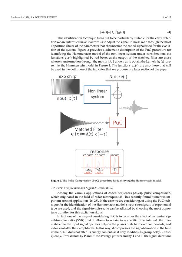
This identification technique turns out to be particularly suitable for the early detec-
tion we are interested in, as it allows us to adjust the signal-to-noise ratio through the
most opportune choice of the parameters that characterize the coded signal used for the
excitation of the system. Figure 2 provides a schematic description of the PuC procedure
for identifying the Hammerstein model of the non-linear system under consideration: the
functions gk (t) highlighted by red boxes at the output of the matched filter are those whose
transformation through the matrix [ Ac ] allows us to obtain the kernels hk (t) present in theMathematics 2021, 9, 850 6 of 14
Hammerstein model in Figure 1. The functions gk (t) are also those that will be used in the
definition of the indicator that we propose in a later section of the paper.
Figure 2. The Pulse Compression (PuC) procedure for identifying the Hammerstein model.
2.2. Pulse Compression and Signal-to-Noise Ratio
Among the various applications of coded sequences [23,24], pulse compression, which
originated in the field of radar techniques [25], has recently found numerous important
areas of application [26–28]. In the case we are considering, of using the PuC technique
for the identification of the Hammerstein model, swept sine signals of exponential type
are used, and the signal-to-noise ratio can be adjusted by choosing the most opportune
duration for this excitation signal.
In fact, one of the ways of considering PuC is to consider the effect of increasing signal-
to-noise ratio (SNR) that it allows to obtain in a specific time interval: the filter matched to
the input signal operates only on the phases of its harmonic components, and it does not
alter their amplitudes. In this way, it compresses the signal duration in the time domain,
but does not alter its energy content, as it only modifies its group delay. Consequently, if
we denote by P and P’ the average powers and by T and T’ the signal durations before and
after compression, we will then have P × T = P’ × T’, from which the average signal power
after compression can be written as P’ = P × (T/T’). This way of expressing the average
power shows that the ratio (T/T’) can be seen as an equivalent power gain. For impulsive
signals, such as that occurring after compression, the duration of the signal is inversely
proportional to their bandwidth: B ∝ 1/T; consequently, in many cases the equivalent
power gain is expressed as TB: if we have an amplifier capable of providing a power of P
[W], after compression in the interval of duration T’ of the compressed signal, we have a
signal equivalent to what we would have had with an amplifier TB times more powerful.
If the noise has the same power, TB therefore translates into a gain in SNR.
2.3. Innovative Indices for Early Damage Detection
Having available accurate modeling techniques makes it possible to define highly
sensitive indicators for the early detection of damage to the structure, based on the non-
linear nature of the response of the system under consideration. We will examine an
indicator, proposed in [22], that has demonstrated excellent characteristics, analyze its
behavior and propose an original indicator.Mathematics 2021, 9, 850 7 of 14
2.3.1. The DI1 : Ratio of the Non-Linear Energy to the Linear Energy
The DI1 damage indicator is based on a brilliant method to separate the linear con-
tribution from the non-linear one. The method is based on the Hammerstein model of
the physical structure: having identified the Hammerstein model of the non-linear system
allows to extract from it an indicator of the degree of non-linearity of the system by separat-
ing the contribution to the output signal due to the branches of the model representing the
non-linear components of the system, and comparing this contribution to the one related
to the branch representing the linear part. In [22], the authors make use of this model to
define, among others, the indicator:
f2 2
S NL ( f ) d f
R
f
DI1 = R1 f 2
, (5)
2
f1 |S L ( f )| d f
where S L ( f ) and S NL ( f ) are, respectively, the Fourier transforms of the response of the
linear branch and the sum of the responses of the non-linear branches of the Hammerstein
model, once identified, when the exponential sine sweep signal is input; f 1 and f 2 are the
extreme frequencies of the exponential sine sweep signal that is used as input to the system
in the phase of identification of the non-linear system, the same signal used as input to the
Hammerstein model, once identified, to estimate the damage index DI1 .
2.3.2. The Proposed Harmonic Index
The definition of an estimator for the degree of non-linearity can only be based on the
separation of the linear and non-linear parts. The good results produced by the damage
index DI1 show that, in this field too, the use of a priori information, in the form of a model
of the structure to be represented, significantly improves the estimation sensitivity.
The aspect that we have considered to focus on in examining the performances of
the estimator, is the degree of immunity to noise of the data collected: the conditions in
which the acquisition of the measurement data take place are in fact very frequently limited
in power, thus noise level overrides small signal variations and this makes it difficult to
detect small differences between the responses of an intact specimen and a faulty one of
the system under examination, in case we are interested in an early manifestation of a
possible defect.
The DI1 technique implies that once the Hammerstein model is identified, it is used
by injecting the noise-affected swept sine signal at its input: the sum of signal and noise is
processed by each of the parallel branches in the model. The sum of the energies of the
output signals from the non-linear branches is divided by the energy of the output signal
from the linear branch: this ratio is the DI1 index. The effect of the input noise, altered by the
processing phases in the different branches of the model, directly reflects on the estimated
value for the DI1 index. This estimator therefore does not make use of the improvements
in the SNR ratio that can be achieved through the PuC technique, even though the PuC
technique was used in the previous Hammerstein model identification phase.
As far as the damage index is concerned, our proposal is therefore to define the
indicator using quantities calculated in the PuC phase, a procedure that is in any case
implemented for the identification of the Hammerstein model: following this approach has
the advantage of using the PuC procedure for two purposes, and furthermore of having a
defect index estimated under more advantageous equivalent SNR conditions.
There is a second argument in support of the potential offered by a damage index
definition based on quantities calculated in the PuC phase, thus considering the signal
u(t) at the output of the matched filter: the estimator proposed in [22] makes use of the
Hammerstein model once identified, and measures the energy of the linear and non-linear
parts of the output signal of the model when an exponential sine sweep signal feeds
into the parallel branch structure: this input signal has, by definition, a spectral energy
distribution strongly unbalanced towards one of the extremes of the covered band: in the
case of a signal with exponentially increasing frequency (up-chirp), the harmonic contentMathematics 2021, 9, 850 8 of 14
is mainly concentrated towards the lowest range of frequencies. Assuming that the noise
superimposed in the measurement phase is assimilable to a Gaussian white noise, it is
evident how the ratio between useful signal and noise is strongly unequal in the different
frequency ranges. This fact makes the estimator proposed in [22] particularly exposed to the
effects of noise in the frequency ranges where the signal-to-noise ratio is less advantageous,
frequency bands that might be particularly important for detecting small defects, which are
important for early detection: it is therefore particularly important to check the sensitivity
and robustness of the estimator in the presence of noise. In order to verify these aspects,
we report in the next paragraph the results of some simulations carried out in a wide range
of signal-to-noise ratios, evaluation including also very low SNR values.
The proposal of a new estimator starts from the above considerations and, being
always based on the Hammerstein model, does not use the energy of the signal at the
model output, separated between linear and non-linear components, but directly the
energy associated to the impulsive functions gk (t) in the vector [ g(t)] which are estimated
during the model identification phase, as reported in equation (3). These functions directly
carry information about the different harmonics that are generated in the response of the
non-linear system; moreover, their estimation, carried out downstream of the matched
filter, compensates in this way the non-uniformity in the energy content of the excitation
signal, which is automatically equalized by the matched filter.
Based on this consideration, we propose the following harmonic index of damages in
the structure:
N R 2
∑k=H2 (gk (t)) dt
HI = , (6)
(g1 (t))2 dt
R
where the integrals are carried out in the time domain, extended to the entire duration of
each gk (t) function.
2.3.3. The Simulated System
The experiments were performed by generating synthetic signals using the same
model used in [22], a model previously proposed and used in [29]. The system that has
been chosen is a one degree of freedom system, of the spring-mass-damper (SMD) type as
shown in Figure 3. The damage in these systems has been introduced through a bi-linear
stiffness k [ x (t)], and allows to simulate in a very simple way a breathing fracture [29]. For
these fractures there is a lower stiffness when the fracture is open than when it is closed.
Consequently, the bi-linear stiffness is defined as follows:
(
kI
k[ x (t)] = . (7)
(1 − α )k I
Figure 3. The one degree of freedom system, of the spring-mass-damper.
In this definition, k I indicates the linear stiffness of the original undamaged system
and the damage parameter of the simulation model is the coefficient α. If α = 0, the stiffness
is fully linear and the system is intact. If α = 1, the stiffness is zero when the fracture is
open, and consequently the system is fully damaged.Mathematics 2021, 9, 850 9 of 14
We have chosen a single-input, single-response (SISO) system whose input is the force
f (t) applied to the mass M; the output is the displacement x (t) of the mass M, as shown
in Figure 3.
The effect of noise, in this case, may affect the quality of the estimation of the gk (t)
functions if the output signal used in the identification phase is affected by additive noise.
3. Experimental Results
In accordance with [22], we generated data from the system defined by relation (7)
using the following parameters: M = 1 [kg], B = 2 [N s/m], and k I = 20 000 [N/m].
An input signal with the characteristics of an exponential sine sweep with increasing
frequency was used to identify the Hammerstein model and subsequently to estimate the
value of the damage indicators under comparison. The resonance frequency of the mechan-
ical system described above is f R = 22.5 [Hz] for the undamaged system. Consequently,
according to [22], we selected the initial frequency f 1 = 2.25 [Hz] and final frequency
f 2 = 225 [Hz]. The duration chosen for the excitation signal was T = 9.36 [s].
The response of this system was simulated within the Mathematica(r) environment.
A zero mean, white Gaussian noise was added to the input of the simulator to consider the
environmental noise. In order to allow a complete comparison with the data reported in
the paper [22], we assumed that the measurement system does not add any perceptible
noise component to the signal detected. The variance of the noise was chosen according to
the desired signal-to-noise ratio: initially the results for SNR of 60 and 30 dB are reported,
as in [22]. Measurements with much higher noise levels were also carried out, such that
the SNR ratio was brought down to a value of 0 dB. Each simulation was performed for
the same range of α damage parameter: the values considered were between α = 0% and
α = 50% for all simulations. For each value of α and for each value of the signal-to-noise
ratio, the simulation was repeated 30 times in order to calculate the mean value and the
standard deviation of each one of the damage estimators under comparison in the presence
of noise.
Figure 4 shows, in the four panels, the trend in the case of SNR = 60 dB and in the
case of SNR = 30 dB of the mean value and the standard deviation (±2σ) of the estimator
of the two damage indicators being compared. The abscissa shows the extent of damage α,
whose value varies between 0% and 50%. The mean value and the standard deviation are
calculated, as in all subsequent cases, on 30 independent tests.
Figure 4. Mean value and standard deviation (±2σ) of the estimators depending on the amount
of damage α. (a) Damage indicator DI1 @ SNR = 60 dB; (b) The proposed damage indicator HI @
SNR = 60 dB; (c) damage indicator DI1 @ SNR = 30 dB; (d) The proposed damage indicator HI @
SNR = 30 dB.Mathematics 2021, 9, 850 10 of 14
At such high levels of the signal-to-noise ratio, and with this type of representation,
the trend of the mean values of each damage indicator in the case of 30 and 60 dB is actually
indistinguishable: both indicators at these noise levels provide very stable indications.
Only a greater variability around the mean value in the case of noise at 30 dB for DI1 can
be seen.
In addition to highlighting the stability of both estimators, Figure 4 shows some
interesting aspects for comparing the two damage indicators: (1) the greater stability of
the estimate obtained with the HI indicator that we propose compared to that with the
DI1 indicator, as can be seen from the significantly lower σ values in the first case; (2) the
more gradual decrease in the value of the estimator as the magnitude of the damage index
α decreases. This latter aspect is particularly interesting if we want useful indications for
early detection of damage, i.e., for low values of α. To analyze this aspect in more detail,
it may be useful to report the same values of Figure 4, panels (c) and (d), in a double
logarithmic scale, in order to better evaluate the regularity of the variation of the trend of
the indicators as α varies, especially in the lower range. In panels (a) and (b) of Figure 5, the
trends of the two indicators in the case of SNR = 30 dB are plotted on a double logarithmic
scale: their comparison shows a flattening of the curve of the DI1 as α decreases, while
the HI indicator decreases in a regular way up to the minimum α values. The HI therefore
shows greater sensitivity than the DI1 to even minimal damage, at the same noise level.
Figure 5. Mean value and standard deviation (±2σ) of the estimators depending on the amount
of damage α. (a) Double logarithmic scale representation of damage indicator DI1 @ SNR = 30 dB;
(b) double
logarithmic scale representation
of the proposed damage indicator HI @ SNR = 30 dB;
σ σ
(c) µ for DI1 @ SNR = 30 dB; (d) µ for HI @ SNR = 30 dB.
Panels (c) and (d) of the same Figure 5 show a comparison of the trends of the ratio
σ
µ between the estimated standard deviation σ and average value µ, plotted as the entity
α of the damage varies: the comparison between the two curves shows for both a value
of the ratio that decreases as the extent of the damage α increases: as expected, a more
evident damage gives rise to more stable estimates. The values of the ratio are however
very different between the two curves, confirming the greater stability of the estimate of
the HI indicator in the presence of noise.
We decided to further investigate the comparison between the two damage indicators
in relation to their sensitivity to small damage, and their ability to provide a reliable
estimated value even in the presence of high noise levels. To this end, we have carried out
further tests in conditions of increasing noise level, down to SNR = 0 dB. The results are
reported in Figures 6–8, relating respectively to SNR values of 10, 5, and 0 dB. The three
Figures 6–8 are organized in the same way as Figure 5: in each, the panels (a) and (b) report,
for the two indicators considered, the average value and the standard deviation, estimatedMathematics 2021, 9, 850 11 of 14
on 30 repetitions, as a function the values of the entity of the damage α. Ineach figure,
σ
panels (c) and (d) show, for the two indicators considered, the trend of the µ ratio as
the extent of the damage parameter α varies. As with all other tests, each σ and µ value is
estimated on 30 independent tests.
Figure 6. Mean value and standard deviation (±2σ) of the estimators depending on the amount
of damage α. (a) Double logarithmic scale representation of damage indicator DI1 @ SNR = 10 dB;
(b) double
logarithmic scale representation
of the proposed damage indicator HI @ SNR = 10 dB;
σ σ
(c) µ for DI1 @ SNR = 10 dB; (d) µ for HI @ SNR = 10 dB.
Figure 7. Mean value and standard deviation (±2σ) of the estimators depending on the amount
of damage α. (a) Double logarithmic scale representation of damage indicator DI1 @ SNR = 5 dB;
(b) double
logarithmic scale representation
of the proposed damage indicator HI @ SNR = 5 dB;
σ σ
(c) µ for DI1 @ SNR = 5 dB; (d) µ for HI @ SNR = 5 dB.
The figures clearly show how, as the noise level increases, the quality of the estimate
for both damage indicators worsens. In particular for SNR equal to 0 dB, both demonstrate
that they are unable to modify their average value as a function of the parameter α. For
SNR equal to 5 dB, the HI indicator we propose shows some, albeit limited, ability to
detect the presence of damage exceeding α = 10%, while the DI1 shows no variation. These
different behaviors of the two damage indicators appears more evident for SNR = 10 dB.Mathematics 2021, 9, 850 12 of 14
Figure 8. Mean value and standard deviation (±2σ) of the estimators depending on the amount
of damage α. (a) Double logarithmic scale representation of damage indicator DI1 @ SNR = 0 dB;
(b) double
logarithmic scale representation
of the proposed damage indicator HI @ SNR = 0 dB;
σ σ
(c) µ for DI1 @ SNR = 0 dB; (d) µ for HI @ SNR = 0 dB.
It is also interesting to observe that the σ value significantly decreases starting from
the α damage values for which its average value µ begins to change, showing that the
defect can be detected by the damage index considered. In all these cases the µσ ratio
relating to the HI indicator that we propose is lower than that relating to the DI1 indicator,
thus showing that, even in conditions of high noise level, the damage HI indicator tends in
any case to be more reliable.
A fundamental aspect which emerges from a comparative analysis of the different
figures describing our experiments is that, in the case of a very low SNR, and especially for
small alterations of this signal due to defects (low α values), neither of the two methods is
able to detect the presence of defects (see for example the curves for SNR = 0 dB: the value
of both indices does not change when the entity of the defect, i.e., the value of α, varies).
On the other hand, when the SNR is extremely high, especially for high α values, the
presence of the defect is so evident that both indicators detect it without problems (see for
example the curves for SNR = 60 or 30 dB: the value of both indices grows with regularity
as α increases, i.e., as the extent of the defect raises).
The comparison between the two indicators is therefore played in verifying which
method is able to detect first (i.e., for a lower α value, SNR being equal) the presence of
defects. We can verify this, for each SNR, by increasing the α value. For very low α values,
none of the indicators does change its value as the size of the defect increases: in fact, the
noise is such, compared to the variations due to the defect, that the estimator does not
change its value, that is, it does not detect the defect. The α value by which the estimator
value begins to increase, evidences the beginning of the sensitivity zone for that indicator.
So, it is not so much the absolute value of the estimator to be relevant, as it is going to
verify for which α value the index begins to modify its value.
For example, the curves for SNR = 5 dB show a substantially constant DI1 for the
whole range, up to α = 50%, while the HI estimator begins to increase its value regularly
starting from α = 13%; further confirmation of this behavior is highlighted by the significant
decrease in the variability of the estimates around their average value starting from the
same values of the α parameter (13%). We have decided to further highlight these aspects,
which weconsider interesting for the comparison, by reporting—for each SNR—the trends
of the µσ ratio as the α varies. Consistently with the observations just made, the trend of
this curve confirms that the HI indicator shows that it detects the presence of defects evenMathematics 2021, 9, 850 13 of 14
in situations in which the DI1 is still made insensitive by the environmental noise present
in the data.
Similar behaviors are found in the case of the curves for SNR = 10 dB, for which the
indicator DI1 enters the sensitivity zone for parameter α = 30%, while the HI indicator we
propose is sensitive to variations in the extent of the defect already for α = 10%.
4. Conclusions
The non-linear techniques appear as a frontier for an improvement of the defect
detention capacity at the early stage of defect formation. We have taken as a reference
the DI1 , a technique that has proved to be effective and we have analyzed it thoroughly
in order to improve its performance in the ability to provide reliable indications even
in the presence of minor defects and in the presence of significant noise levels during
data acquisition.
We have verified the possibility of using parameters that the DI1 technique already
considered in a preliminary phase, and we have used them to define the harmonic index
HI, a novel damage indicator. The experimental tests carried out by repeating the same
experiment reported in the technical literature, in addition to finding the same values for
the reference index DI1 , made it possible to find that the hypotheses of greater robustness
to noise of the new proposed HI indicator are verified.
An accurate analysis of the trend of the two indicators for low damage values also
highlighted a greater sensitivity of the new HI indicator for small damage, an aspect that is
particularly important if one is interested in early detection of defects. Finally, we carried
out numerous tests with remarkably high noise levels, to compare the robustness level
of the two damage indicators and to obtain indications of the operating limits of both
damage indicators. In addition, the new HI indicator we proposed has shown to have
greater sensitivity and to provide indications less affected by the measurement noise.
The aim of the present work was to report the results of evaluations comparing the
innovative indicator we defined with an indicator of very good performance that was
already available in the technical literature. The comparisons had to be made under the same
operating conditions, and this was done accurately using data obtained through simulations.
The extremely comforting results in terms of the stability of the estimated value
as the extent α of the damage varies, and the robustness with respect to measurement
noise, push this research activity towards carrying out a verification of the technique on
experimentally measured data: this will allow a further comparison with other techniques
of early damage detection.
Author Contributions: Conceptualization, P.B. and M.C.; Formal analysis, P.B. and M.C.; Software,
P.B. and M.C.; Writing—original draft, P.B. and M.C. Both authors contributed substantially to the
present work and have read and agreed to the published version of the manuscript.
Funding: This research received no external funding.
Institutional Review Board Statement: Not applicable.
Informed Consent Statement: Not applicable.
Data Availability Statement: Experiments carried out with data generated by the described syn-
thetic model.
Acknowledgments: The authors thank the editor of this Special Issue for the encouragement and
patient support.
Conflicts of Interest: The authors declare no conflict of interest.
References
1. Tsyfansky, S.; Beresnevich, V. Detection of fatigue cracks in flexible geometrically non-linear bars by vibration monitoring. J. Sound
Vib. 1998, 213, 159–168. [CrossRef]
2. Bayma, R.S.; Zhu, Y.; Lang, Z.Q. The analysis of non-linear systems in the frequency domain using non-linear output frequency
response functions. Automatica 2018, 94, 452–457. [CrossRef]Mathematics 2021, 9, 850 14 of 14
3. Su, Z.; Zhou, C.; Hong, M.; Cheng, L.; Wang, Q.; Qing, X. Acousto-ultrasonics-based fatigue damage characterization: Linear
versus non-linear signal features. Mech. Syst. Signal Process. 2014, 45, 225–239. [CrossRef]
4. Broda, D.; Staszewski, W.J.; Martowicz, A.; Uhl, T.; Silberschmidt, V.V. Modelling of non-linear crack–wave interactions for
damage detection based on ultrasound—A review. J. Sound Vib. 2014, 333, 1097–1118. [CrossRef]
5. Burrascano, P.; Laureti, S.; Ricci, M. Harmonic Distortion Estimate for Damage Detection. In Proceedings of the NAECON
2018-IEEE National Aerospace and Electronics Conference, Dayton, OH, USA, 23–26 July 2018; pp. 274–279.
6. Sutin, A.M.; Johnson, P.A. Non-linear elastic wave NDE II. Non-linear wave modulation spectroscopy and non-linear time reversed
acoustics. In AIP Conference Proceedings; American Institute of Physics: College Park, MD, USA, 2005; Volume 760, pp. 385–392.
7. Bruno, C.L.E.; Gliozzi, A.S.; Scalerandi, M.; Antonaci, P. Analysis of elastic non-linearity using the scaling subtraction method.
Phys. Rev. B 2009, 79, 064108. [CrossRef]
8. Burrascano, P.; Di Bella, A.; Gliozzi, A.; Laureti, S.; Ricci, M.; Rizwan, M.K.; Tortello, M. A comparison of scaling subtraction and
pulse compression methods for the analysis of elastic non-linearity. In Proceedings of Meetings on Acoustics ICU; American Institute
of Physics: College Park, MD, USA, 2019; Volume 38, p. 065013.
9. Novak, A.; Bentahar, M.; Tournat, V.; El Guerjouma, R.; Simon, L. Non-linear acoustic characterization of micro-damaged
materials through higher harmonic resonance analysis. Ndt E Int. 2012, 45, 1–8. [CrossRef]
10. Mechri, C.; Scalerandi, M.; Bentahar, M. Separation of damping and velocity strain dependencies using an ultrasonic monochro-
matic excitation. Phys. Rev. Appl. 2019, 11, 054050. [CrossRef]
11. Donskoy, D.; Sutin, A.; Ekimov, A. Non-linear acoustic interaction on contact interfaces and its use for non-destructive testing.
Ndt E Int. 2001, 34, 231–238. [CrossRef]
12. Metya, A.K.; Tarafder, S.; Balasubramaniam, K. Non-linear lamb wave mixing for assessing localized deformation during creep.
Ndt E Int. 2018, 98, 89–94. [CrossRef]
13. Sun, M.; Xiang, Y.; Deng, M.; Tang, B.; Zhu, W.; Xuan, F.Z. Experimental and numerical investigations of non-linear interaction of
counter-propagating lamb waves. Appl. Phys. Lett. 2019, 114, 011902. [CrossRef]
14. Climent-Llorca, M.Á.; Miró-Oca, M.; Poveda-Martínez, P.; Ramis-Soriano, J. Use of higher-harmonic and intermodulation
generation of ultrasonic waves to detecting cracks due to steel corrosion in reinforced cement mortar. Int. J. Concr. Struct. Mater.
2020, 14, 1–17. [CrossRef]
15. Chen, J.; Xu, Z.; Yu, Y.; Yao, Y. Experimental characterization of granite damage using non-linear ultrasonic techniques. Ndt E Int.
2014, 67, 10–16. [CrossRef]
16. Sound System Equipment—Part 5: Loudspeakers; IEC 60268-5; International Electrotechnical Commission: Geneva, Switzerland,
2003.
17. Kay, S.M.; Marple, S.L. Spectrum analysis—A modern perspective. Proc. IEEE 1981, 69, 1380–1419. [CrossRef]
18. Daniell, P.J.; Volterra, V. The theory of functionals and of integral and integro-differential equations. Math. Gaz. 1932, 16, 59.
[CrossRef]
19. Schetzen, M. The Volterra and Wiener Theories of Non-Linear Systems; Wiley: Hoboken, NJ, USA, 1980.
20. Schoukens, J.; Pintelon, R.; Dobrowiecki, T. Linear modeling in the presence of non-linear distortions. IEEE Trans. Instrum. Meas.
2002, 51, 786–792. [CrossRef]
21. Novak, A.; Simon, L.; Kadlec, F.; Lotton, P. Non-linear system identification using exponential swept-sine signal. IEEE Trans.
Instrum. Meas. 2010, 59, 2220–2229. [CrossRef]
22. Rébillat, M.; Hajrya, R.; Mechbal, N. Non-linear structural damage detection based on cascade of Hammerstein models. Mech.
Syst. Signal Process. 2014, 48, 247–259. [CrossRef]
23. Carpentieri, M.; Ricci, M.; Burrascano, P.; Torres, L.; Finocchio, G. Wideband microwave signal to trigger fast switching processes
in magnetic tunnel junctions. J. Appl. Phys. 2012, 111, 07C909. [CrossRef]
24. Carpentieri, M.; Ricci, M.; Burrascano, P.; Torres, L.; Finocchio, G. Noise-like sequences to resonant excite the writing of a
universal memory based on spin-transfer-torque MRAM. IEEE Trans. Magn. 2012, 48, 2407–2414. [CrossRef]
25. Cook, C. Pulse compression-key to more efficient radar transmission. Proc. IRE 1960, 48, 310–316. [CrossRef]
26. Laureti, S.; Colantonio, C.; Burrascano, P.; Melis, M.; Calabrò, G.; Malekmohammadi, H.; Sfarra, S.; Ricci, M.; Pelosi, C. Development
of integrated innovative techniques for paintings examination: The case studies of The Resurrection of Christ attributed to Andrea
Mantegna and the Crucifixion of Viterbo attributed to Michelangelo’s workshop. J. Cult. Herit. 2019, 40, 1–16. [CrossRef]
27. Burrascano, P.; Ricci, M.; Battaglini, L.; Senni, L. Non-linear convolution and fourier series coefficients estimate. In Proceedings
of the 2014 IEEE China Summit & International Conference on Signal and Information Processing (ChinaSIP), Xi’an, China,
9–13 July 2014; pp. 728–732.
28. Burrascano, P.; Laureti, S.; Ricci, M.; Terenzi, A.; Cecchi, S.; Spinsante, S.; Piazza, F. A swept-sine pulse compression procedure for
an effective measurement of intermodulation distortion. IEEE Trans. Instrum. Meas. 2019, 69, 1708–1719. [CrossRef]
29. Andreaus, U.; Baragatti, P. Cracked beam identification by numerically analysing the non-linear behaviour of the harmonically
forced response. J. Sound Vib. 2011, 330, 721–742. [CrossRef]You can also read