Coevolution Pigeon-Inspired Optimization with Cooperation-Competition Mechanism for Multi-UAV Cooperative Region Search - MDPI
←
→
Page content transcription
If your browser does not render page correctly, please read the page content below
applied
           sciences
Article
Coevolution Pigeon-Inspired Optimization with
Cooperation-Competition Mechanism for
Multi-UAV Cooperative Region Search
Delin Luo 1, * , Jiang Shao 1 , Yang Xu 1 , Yancheng You 1 and Haibin Duan 2,3
 1    School of Aerospace Engineering, Xiamen University, Xiamen 361005, China;
      shaojiang@stu.xmu.edu.cn (J.S.); xuyang0108@xmu.edu.cn (Y.X.);
      yancheng.you@xmu.edu.cn (Y.Y.)
 2    School of Automation Science and Electrical Engineering, Beihang University, Beijing 100191, China;
      hbduan@buaa.edu.cn
 3    State Key Laboratory of Virtual Reality Technology and Systems, Beihang University, Beijing 100191, China
 *    Correspondence: luodelin1204@xmu.edu.cn

 Received: 19 January 2019; Accepted: 21 February 2019; Published: 26 February 2019

 Featured Application: Authors are encouraged to provide a concise description of the specific
 application or a potential application of the work. This section is not mandatory.

 Abstract: In this paper, a dynamic two-stage closed search (DTSCS) scheme for the unmanned aerial
 vehicle (UAV) cooperative region search is designed, which satisfies the range constraint (RC) and
 orientation constraint (OC). The closed trajectory is composed of two coupling stages, the search
 stage and the return stage. The position and orientation at the end of the search stage are the starting
 cell and orientation of the return stage. In the first stage, a coevolution pigeon-inspired optimization
 (CPIO) algorithm based on the cooperation-competition mechanism is proposed for multi-UAV
 cooperative search. In the return stage, inspired by region searching and trajectory tracking, a search
 tracking (ST) approach is presented to obtain the lowest-cost path under OC. The simulation results
 show that: (i) Np = 5 is the best prediction time step. (ii) CPIO algorithm performs better than the
 compared intelligent algorithms in region searching. (iii) ST has high tracking performance than
 other algorithms. (iv) The DTSCS scheme enables every UAV to make the best use of its fuel to cover
 more region and return to the airport within the RC, and the average range utilization of UAVs is
 97% under the 3OC.

 Keywords: multi-UAV cooperative search; dynamic two-stage scheme; closed search trajectory; range
 constraint; orientation constraint; coevolution pigeon-inspired optimization; cooperation-competition
 mechanism; the lowest-cost path

1. Introduction
     In the wide-area, complex and changeable environment, multiple unmanned aerial vehicles
(UAVs) cooperative control is a critical research field [1–4] of unmanned system. In particular,
multi-UAV cooperative search (MUCS) can be applied to prevent forest fires, patrol the border and
probe potential safety hazards in cities and other aspects. Therefore, the study of MUCS strategy has
practical significance. In [5], Sujit uses k-shortest path algorithm to search the target in an uncertain
environment, but this algorithm cannot adapt to the situation that the edge weights of the search cell
changes with the number of UAV passes. In [6], Bertuccelli models the uncertainty in the environment
as the prior probabilities in the region and uses the Beta distribution to predict the minimum number
of times required by UAV to search the target. This method, however, only considers a single UAV.

Appl. Sci. 2019, 9, 827; doi:10.3390/app9050827                                  www.mdpi.com/journal/applsci
Appl. Sci. 2019, 9, 827 2 of 20
Riehl transforms MUCS into a finite sequence of updates to a dynamic graph via sampling region
with a high probability of target existence in [7], but ignores the orientation constraint (OC) of UAV.
In [8], Tian maps the search rewards of the target to fitness function and proposes a coevolution genetic
algorithm to search the random target under the OC of UAV. In [9], Hu designs a multi-agent mapping
fusion scheme based on distributed control, which converges the individual search probability of agent
to the whole searching region. Nevertheless, this method does not take into account the impacts of
environmental conditions.
Currently, almost all achievements on MUCS have mentioned that the range limits the application
of UAV. To our knowledge, however, there is no study of the search strategies of MUCS under the
range constraints (RC). The motivation of this paper is to present a new search strategy considering
the range constraint (RC) and the OC. The search path of UAV under RC should be a closed trajectory.
UAVs set out from the airports and need to return to their respective airports after completing the
search task. The search algorithm based on an intelligent algorithm has been proved to be superior to
the traditional optimization algorithm in [10–12]. Intelligent algorithms start the optimization with a
series of possible solutions, and their performances depend primarily on the parameter initializations.
Therefore, the constant parameters are not entirely consistent with the evolutionary spirit of the
algorithm itself [13–15]. The results of optimization may be premature, divergent or locally optimal.
Duan presents the pigeon-inspired optimization (PIO) algorithm based on a dynamic size of solution
agents in [16]. Map and compass operator and landmark operator are used respectively by the distance
of the pigeons from the target. Although there are only two switching operators, the optimization
ability of PIO has been verified to be better than other heuristic algorithms in many applications [17–19].
The grid map can accurately describe the size, location, and shape of obstacles. Eight non-obstacle
neighbor cells are reachable nodes for every cell. Its center is the allowed waypoint [20,21].
The lowest-cost path in grid model corresponding to finding a suitable sequence of cells to move the
UAV from the original cell to a goal cell such that its total accumulated expenditure is minimized.
The least-cost path solved by Dijkstra algorithm [22] or A* algorithm [23] does not take into account
the OC of the UAV. It is assumed that the cells sequence of the lowest path a without the OC is
P a ( L a ) = { L a (1), ..., L a (h), ..., L a ( Na )}(h = 1, ..., Na ), in which L a (h) is the cell that path a contains.
After adding the OC, if an element of P a ( L a ) is not in the feasible region, path a will become a illegal
path. Therefore, A* algorithm and other algorithms cannot find the lowest-cost path under the OC.
Our contributions: (i) We apply the concept of the closed search to MUCS for the first time, and
design a dynamic two-stage closed search (DTSCS) scheme to realize the closed path search of UAV.
The first stage is the search stage, and the second stage is the return stage. The pose, position and
orientation, at the end of the search stage is the starting pose of the return stage. (ii) Inspired by
the cooperation-competition relationship between subgroups within a population in nature, a CPIO
algorithm based on the cooperation-competition mechanism is used as the search algorithm for MUCS
in the first stage. Every subgroup pigeons is abstracted as one UAV. The cooperation-competition
relationship between pigeons reflects the cooperative relationship between UAVs. (iii) In the second
stage, a search tracking approach (ST) is proposed. The cells containing in the lowest-cost path without
the OC are modeled as the key regions in the region searching. The basic PIO algorithm is used to
obtain the lowest-cost path from the starting point to the goal point which satisfies the OC. Maximizing
search rewards is equivalent to minimizing tracking errors.
The rest of the paper is organized as follows. Section 2 introduces the concept of the closed path
and the basics of region searching. In Section 3, A CPIO algorithm based on the cooperation-competition
mechanism is proposed for MUCS. A ST approach is given to obtain the lowest-cost path with the OC
in Section 4. Section 5 describes the DTSCS scheme. Numerical simulations and analysis are drawn in
Section 6. Concluding remarks are given in the final section.Appl. Sci. 2019, 9, 827 3 of 20
2. Problem Formulation
The searching region is usually divided into grid cells. The target existence probability (TEP)
represents the probability of target existence in a cell. Environmental uncertainty (EU) indicates the
degree to which UAVs do not know about the environment. These two variables are regarded as prior
information. Every cell is modeled as the key or non-key region, and then the search probability graph
of the whole searching region is formed. UAVs accomplish the search task via environment perception
and information interaction. This section includes three parts: the environment model, UAV kinematic
model and the analysis of UAV closed search.
2.1. Region Searching Model
This subsection describes the basic mathematical model of region searching. Firstly, rasterizing
the searching region, and then the environment information is modeled as the prior probability
information. The TEP in the whole search environment is updated by Bayesian rule. And the
environmental uncertainty of every cell is updated according to search number of UAVs.
2.1.1. Environment Modeling
UAVs are assumed to fly on a fixed plane above the searching region. M UAVs search Nt targets.
The searching region R is uniformly divided into L x · Ly cells:
R = {C (m, n) | m = 1, 2, ..., L x ; n = 1, 2, ..., Ly }, (1)
where C (m, n) is the coordinate of cell (m, n). The side length of a cell is the unit length. Discretizing
searching time of U AVi (i = 1, 2, ..., M ), U AVi can search a cell in one time step [24,25]. The real-time
position of U AVi can be described by the geometric center of the cell it searches.
2.1.2. Probability Map Update
It is known that the TEP Pem,n (k) ∈ [0, 1] and the EU χm,n m,n
e ( k ) ∈ [0, 1]. If 0 ≤ Pe ( k ) ≤ 0.3
m,n m,n
and 0 ≤ χe (k) ≤ 0.3, the cell (m, n) is modeled as a known region. If 0.3 < Pe (k) ≤ 0.7 and
0.3 < χem,n (k) ≤ 0.7, the cell (m, n) is modeled as a non-key region. And if 0.7 < Pem,n (k ) ≤ 1 and
0.7 < χem,n (k) ≤ 1, the cell (m, n) is modeled as a key region. Dangerous areas, such as hostile radar
detection regions, peaks, etc., are designated as no-fly zones. Bayesian rule is used to update whether a
cell exists a target [26]. The update equations for the probability that a target exists but is not detected
and that the target does not exist but is reported are written as follows:
Pem,n (k ) Pcm,n (k)
Pem,n (k + 1) = , (2)
( Pcm,n (k) − Pfm,n (k )) Pem,n (k ) + Pfm,n (k)
Pem,n (k )(1 − Pcm,n (k ))
Pem,n (k + 1) = , (3)
( Pfm,n (k) −Pcm,n (k )) Pem,n (k) + 1 − Pfm,n (k)
where Pcm,n (k) ∈ [0, 1] is the detection probability of the airborne sensor to the target [27]. Pfm,n (k) ∈
[0, 1] is the false alarm rate, which indicates the probability that there is no target in the cell but a target
is reported. χem,n (k ) decreases with the search number of UAVs, satisfying the following equation:
1
χm,n
e ( k + 1) = N f (m,n)
χm,n
e ( k ), (4)
2
where N f (m, n) ∈ N is the number of times that a cell (m, n) searched by UAVs.Appl. Sci. 2019, 9, 827 4 of 20
2.2. UAV Kinematic Model
The kinematic model of U AVi with constant velocity and OC is obtained as follows:
ẋi (t) = vi (t) cos θi (t),
ẏi (t) = vi (t) sin θi (t),
ẏi (t) = 0, (5)
θ̇i (t) ≤ ε i ,
v̇i (t) = 0,
where ( xi (t), yi (t), zi (t)) is the position of U AVi , vi is its velocity. θi is course angle. The fourth term sets
the constraint on the angle rate, which cannot exceed ε i . In the grid map, U AVi can only move to one
of its eight neighbor cells at a time step, corresponding to the heading Di (k ) = {0, 1, 2, 3, 4, 5, 6, 7} [28].
Definition 1. (D-orientation constraint, DOC). In the grid map, The degree of freedom of the heading in
which the UAV is allowed to walk in the next time step is D.
A slow-moving robot usually satisfies 8OC (equivalent to no constraint ) or 4OC , as shown in
Figure 1a,b. The fast UAV can not turn backward or turn vertically during flying. Therefore, it is
subject to 3OC: go straight (0◦ ), turn left (45◦ ), and turn right (−45◦ ), which can be seen in Figure 1c.
The orientation of the next time step of U AVi can be summarized as follows:
Di (k + 1) = {( Di (k) − 1) mod 8, Di (k) mod 8, ( Di (k) + 1) mod 8}. (6)
Figure 1. OC of motion: (a) 8OC; (b) 4OC; (c) 3OC.
2.3. Preliminary Analysis
In the research of MUCS, we always discuss the cooperative search strategy under the assumption
that there is enough fuel, which is not consistent with the actual situation. Every UAV sets out from
the airport and returns to its airport after completing the search task. The flight path is a closed track.
We divide the closed search into two stages: search stage and return stage.
2.3.1. Closed Path Search
Definition 2. (Closed path). According to the definition of the loop in the directed graph, a closed path is a
flight trajectory of a UAV starting form an airport to carry out task and returning back to the same airport.Appl. Sci. 2019, 9, 827 5 of 20
The closed search in this paper is different from the traveling salesman problem, which to find a
solution that traverses all the reachable nodes from the starting point and returns to the starting point
with the least travel cost. In this paper, the closed search refers to the closed path that UAV returns to
the airport after completing the search task in the grid map.
Rasterizing searing region is consistent with discretizing searching time, so the RC of UAV is
equated with its searching time limit. The closed path of the UAV under the RC should be composed
of two stages: (1) search stage; (2) return stage. Long searching time means that UAV has a limited
time to return and may not even return on time. And the short searching time means that the UAV can
not effectively complete the search task. Ideally, the UAV would return to the airport at the time step
when it is running out of fuel.
2.3.2. Search Stage
UAVs accomplish the search task via environment perception and information interaction.
The principles of MUCS should include the following:
• Get the maximum TEP
• Acquire the maximum reduction of EU
• Avoid UAVs repeatedly searching the same cell
• Prohibit collisions between UAVs
• Fly as far away from the airport as possible to search more unknown cells
• Avoid searching for locally highly remunerated sequences of cells
2.3.3. Return Stage
Definition 3. (The lowest path with D-orientation constraint). The solution that the UAV seeks from
origin to the goal cell with the smallest travel cost under the OC.
The search strategy is no longer considered in the return stage. Our goal is to find a safe and
collision-free lowest path under the OC. This path starts with the current cell and orientation and ends
at the airport.
For the closed search, the primary purpose of this paper is to solve the following three problems:
(1) Set the time step for UAV to return to the airport; (2) Maximize search rewards in the search stage;
(3) The purpose of the return phase is to obtain a shortest path that satisfies the OC.
3. CPIO Algorithm with Cooperation-Competition Mechanism
According to the principle of cooperative search discussed above, we design the reward function
of MUCS and regard it as the fitness function of PIO. In [8,29,30] coevolution genetic algorithm
(GA) is applied to multi-robot platform to find the optimal solution through the cooperation among
robots. In some conditions, the optimal solutions of every robots may sometimes be mutually
exclusive. This conflict is consistent with the competition of subgroups in nature. Inspired by the
cooperation-competition relationship between subgroups within a biological community in nature,
a CPIO algorithm is used as the search heuristics for MUCS in the search stage. The optimal solution
obtained via the CPIO algorithm is the position of a target, which is consistent with the attribute of
region searching.
3.1. Design Reward Function
The MUCS process is modeled as a multiobjective nonlinear programming function with RC, OC,
no-fly zone and collision free and the model is given in Equations (7) and (8):
Np Np Np Np
J1 = ω1 ∑ Pem,n (k + q) + ω2 ∑ ∆χm,n
e ( k + q ) + ω3 ∑ Fr (k + q) + ω4 ∑ Fa (k + q), (7)
q =1 q =1 q =1 q =1Appl. Sci. 2019, 9, 827 6 of 20
Rc ∈ R,
D (k + 1) = {( D (k ) − 1) mod 8, D (k) mod 8, (D (k) + 1) mod 8},
i i i i
s.t. (8)
Ti,1 (k + 1) < Ti ,
dij (k), ..., dij (k + Np ) > 0,
where ω1 , ω2 , ω3 , ω4 are weighting factors, which satisfy ω1 , ω2 , ω3 , ω4 ∈ (0, 1) and ω1 + ω2 + ω3 +
ω4 = 1. Rc is the searchable
q i,1 ( k ) and Ti are the searching time and the range of U AVi
region in R. Tq
respectively. dij (k) = ( xi (k) − x j (k))2 + (yi (k) − y j (k))2 denotes the Euclidean distance of U AVi
and U AVj . Np ≥ 1 is a positive integer. The first and second terms of the J1 are designed to maximize
search rewards, which corresponding to the first and second terms of the principles. The reduction of
EU of the cell (m, n) can be defined as follows:
∆χm,n m,n m,n
e ( k ) = χ e ( k + 1) − χ e ( k ). (9)
The third of the J1 is consistent with the fourth of the principles and is designed to avoid collision
between UAVs: √
−100,
dmin (k) ≤ 2,
Fr (k) = 1 (10)
− dmin (k)
√
e , d (k) > 2, min
where dmin (k) is the minimum element of the dij (k) at time step k, and dij (k) is given√in Appendix A
Equation (A1). When the distance between any two UAVs is less than or equal to 2 unit lengths,
the reward of this term will be −100. And then the rewards of J1 will also be negative. U AVi can only
choose to search cells away from other UAVs. With regard to the fourth term of the J1 , it implies that
the further away U AVi is from the airport, the more rewards it obtains (principle 5):
1
−
Fa (k ) = e d∑ (k ) , (11)
where d∑ (k) is the sum of all the elements in dih (k), which is written in Appendix A Equation (A2).
Definition 4. (Np -step-ahead prediction, Np SAP). Learning from the idea of rolling optimization in model
predictive control theory [31]. In each term of J1 designed in Equation (7), the rewards of the reachable cells to be
calculated is not only the next time step, but also the next Np time steps.
Remark 1. Although n steps are predicted in advance each time, U AVi flies forward only one-time step.
The series of reachable waypoints of Np SAP of U AVi maps the predicted cells sequence Ei (k) =
{Li (k + 1), ..., Li (k + q), ..., Li (k + Np )}(q = 1, ..., Np ) from the step (k + 1) to the future time step
(k + Np ), which is based on the present position Li (k) at time k. The reachable cells included in 3SAP
construct an expanding tree, as shown in Figure 2a. Obviously, the expanding tree generated by
Np SAP contains 3 Np alternative paths and the l-th path can be illustrated as:
Pil (k) = { Lil (k + 1), ..., Lil (k + q), ..., Lil (k + Np )}, (12)
where Lil (k + q) ∈ Li (k + q).Appl. Sci. 2019, 9, 827 7 of 20
45o J 1,1 k " 3 # 1!
path1
!
J 1,1 k " 2 # 1
path2
!
J 1,1 k " 1 # 1
Li k " 1 !
Li k ! !
J 1,2 k " 3 # 3
Li k " 2 ! !
J 1,2 k " 2 # 0.5
Li k " 3 ! !
J 1,2 k " 1 # 0.5
(a) (b)
Figure 2. Schematic diagram of Np SAP: (a) Np = 3; (b) Np SAP to avoid greedy thought.
The positive aspects of Np SAP include:
• Avoid greedy thought corresponding to the sixth term of principles referred in Section 2.3.2
• Circumvent the no-fly zone ahead of time and continue to search the key region
• Prohibit collision between UAVs
• Reduce the impact of communication delays
As given in Figure 2b, Comparing the reward of path1 and path2 , if Np = 1, J1,1 (k + 1) >
J1,2 (k + 1), the path1 is chosen at this time step. Else if Np = 3, J1,1 (k + 1) + J1,1 (k + 2) + J1,1 (k + 3) >
J1,2 (k + 1) + J1,2 (k + 2) + J1,2 (k + 3), the path2 will be chosen. For an extreme situation, if Np = Ti,1 ,
the path with the largest reward in Ei (k) must be the optimal path in the whole search process. As Np
grows, the number of paths increases exponentially. Therefore, we use PIO algorithm to find the
optimal solution that is difficult for conventional optimization algorithms.
3.2. Overview of Basic PIO
Inspired by natural phenomenon of the autonomous homing behavior of pigeon swarms, Duan
proposes the PIO algorithm in [14], which the optimization process can be divided into two operators
based on the distance of the pigeons from the destination.
Operator 1: Map and compass operator
During the prometaphase of the search, pigeons is far away from the goal. The real-time
information of the sun is abstracted into map and compass operator to adjust the flight orientation,
which is a rough navigation process. Suppose the number of pigeons is C1 . The position and velocity
of pigeon a , ( a = 1, 2, ..., C1 ) in the two-dimensional (2D) plane is expressed as:
(
L a = [ x a , y a ],
(13)
Va = [v x,a , vy,a ].
The renewal equations of position and velocity are:
(
Lua = Lua −1 + Vau ,
(14)
Vau = Vau−1 e− R p ·u + rand( Lbest − Lua −1 ),
where u = 1, 2, ..., Nc1 is the current iteration number. R p is the coefficient of the map and compass
operator. rand is a random number from 0 to 1. Lbest denotes the position of the pigeon closest to the
goal in the pigeons in iteration u − 1. After Nc1 iterations, the rough navigation stage is completed.
PIO algorithm enters the second stage of optimization.Appl. Sci. 2019, 9, 827 8 of 20
Operator 2: Landmark operator
When the pigeons arrive near the target, the PIO algorithm switches to the landmark operator.
The landmark information of the nearby environment will provide precise guidance information.
The speed of the pigeon does not change at this stage, while the position is updated:
C2v−1
∑ Lvk −1 · f itness( Lva −1 )
−1 a =1
Lvcenter = , (15)
C2v−1
C2v−1 · ∑ f itness( Lva −1 )
a =1
Lva = Lva −1 + rand · ( Lvcenter
−1
− Lva −1 ), (16)
C2v−1
where v = 1, 2, ..., Nc2 is the current iteration number. C2v = is the number of pigeons in v
2
v −1
iteration. Lcenter denotes the position of the central pigeon in v − 1 iteration. f itness(·) is the fitness
function. The optimal solution will be obtained after Operator 2 is performed Nc2 iterations.
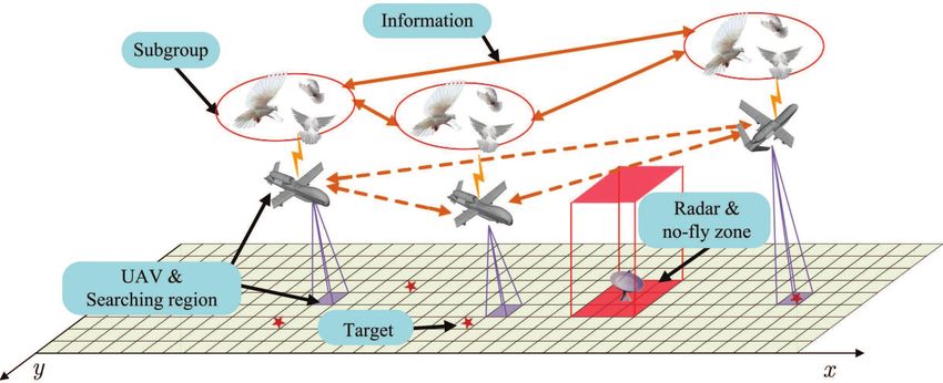
3.3. CPIO and Cooperative Search
In biology, a population may divide into some subgroups [32,33]. In the face of natural enemies,
the subgroups will cooperate to resist. Nevertheless, they also compete with each other in the interests
of food, mating, territory, and so on. Cooperation and competition make the population survive and
evolve better. To simulate these natural behaviors, UAVs work together to complete the search task
via information interaction, in the mean time UAVs compete with each other to search the specific
vital cells. We propose a CPIO algorithm based on the cooperation-competition mechanism as the
search algorithm for MUCS, as shown in Figure 3. In which, one subgroup pigeons is abstracted as one
UAV. The cooperation-competition relationship between pigeons reflects the cooperative relationship
between UAVs.
MUCS based on CPIO is composed of three parts: CPIO, UAVs, and environment model.
The principle of which is shown in Figure 4. In the CPIO module, the initial information of the
environment, the environment information detected by the UAVs and the real-time pose signals of the
UAVs are modeled as prior information. This information is then transmitted to the reward function
J1 . Subgroupi transforms the optimal solution obtained by the cooperative-competitive mechanism
into discrete flight signals. And these signals will be transmitted to U AVi at each time step. Thus,
the cooperation-competition mechanism can be described as follows:
Cooperation mechanism
• Get the maximum Pem,n (k) and the maximum ∆χm,n e (k)
• Stay away from airports and search for more unknown regions
• Avoid searching locally highly remunerated cells
Competition mechanism
• Forbid UAVs to search for the same cell at the same time step
• Avoid UAVs repeatedly searching the same cell
• Stay away from other UAVs to search more unknown cells
Under all constraints, the subgroup that maximizes the total rewards will win. Cooperation and
competition are not entirely opposed to each other. The winning subgroup will search the controversial
cell, and the other subgroups compete to search other cells. The result of the competition mechanism
is consistent with the original intention of the cooperation mechanism.Appl. Sci. 2019, 9, 827 9 of 20
Figure 3. CPIO algorithm for MUCS.
Prior information UAV1
Subgroup1
Competition-Cooperation
Maximize Pe m,n k ! Collision free Subgroup2
UAV2
Maximize reduction of e
m ,n
k ! No-fly zone
No repeated search Range constraint UAVi
Unsearched region Subgroupi
Orientation constraint
Subject to
Reward function Constraints UAVs
Pigeons
CPIO No-fly zoneˈ Key regionˈ Non-key regionˈ Known region Environment model R
Figure 4. Schematic diagram of MUCS based on cooperation-competition mechanism.
Let f itness(·) = J1 , thus Equation (15) can be transformed into:
C2v−1
∑ Lvk −1 · J1 ( Lva −1 )
−1 a =1
Lvcenter = . (17)
C2v−1
C2v−1 · ∑ J1 ( Lva −1 )
a =1
In the searching region, Lua and Lva are neighbor cells of Lua −1 and Lva −1 , respectively. Under the
constraint of Equation (6), the position (orientation) in the PIO algorithm can be expressed as:
Lua = {( Lua −1 − 1) mod 8, Lua −1 mod 8, ( Lua −1 + 1) mod 8}, (18)
Lva = {( Lua −1 − 1) mod 8, Lva −1 mod 8, ( Lva −1 + 1) mod 8} = Lua −1 + rand · ( Lucenter
−1
− Lua −1 ). (19)
The MUCS process based on the CPIO algorithm can be expressed as Algorithm 1.Appl. Sci. 2019, 9, 827 10 of 20
Algorithm 1 MUCS based on CPIO algorithm
Input: Initializing environmental information and pose information of U AVi .
Output: The searching trajectory of every UAV and its searching time steps Ti,1 (k).
1: begin:
2: for k = 1, ..., Ti do
3: Predict N time steps in advance, and get the alternative paths.
4: Delete the paths that does not satisfy Equation (8).
5: Use the CPIO algorithm to find the path with the highest fitness value among the remaining paths.
6: while U AVi receives the return order, U AVi returns to the airport.
7: Record the searching trajectory and searching time steps Ti,1 (k) when U AVi returns.
8: end while
9: end for
10: end
4. ST Approach
Inspired by the knowledge of cooperative search and trajectory tracking [34,35], we propose the
ST approach. The lowest path a without the OC of motion is mapped to a trajectory to be followed, and
the cells it passes through are modeled as the key regions. Other blank cells are shaped as non-key
regions, and obstacles are designed as no-fly zones. The input signal is the orientation sequence to
maximize the search rewards of U AVi . The process of tracking path a is the same as that of a UAV
searching from the starting cell to the goal cell. Since the ST approach is only applied to a single UAV,
there is no need to consider the cooperation-competition relationship between UAVs. ST approach
based on basic PIO algorithm consists of four operators.
Operator 1: Obtain path a
We use A* algorithm [23] to find path a , and A* algorithm can be simplified as the following steps:
Step 1: Specify the OC for the UAV.
Step 2: Design a cost function f (m, n) = g(m, n) + h(m, n), where g(m, n) denotes the movement
cost: corresponds to the expenditure of moving the current position (m, n) to other cell moved
into the neighbor. h(m, n) denotes the heuristic cost: corresponds to the expenditure of changing
from current cell to goal cell. When g(m, n) = 0, A* algorithm degenerates to Dijkstra algorithm.
When h(m, n) = 0, A * algorithm degenerates to greedy best first search algorithm.
Step 3: Estimate total expenditure h(m, n) and change to the cell with the least cost.
Step 4: Repeat Step 3 until the goal cell is reached.
Step 5: When reaching the goal, choose the final path with least cost.
Operator 2: Mark key cells
Referring to the concept of the TEP in the region searching, the blank cells are set as the non-key
m,n
regions, which implies Pe,i (k) = 0. The cells that the path of U AVi path a,i passes through are marked
m,n
as the key regions, and their Pe,i (k) are denoted as follows:
1
, 1 < si < Nm,i , N f ,i = 0,
5
si = Nm,i , N f ,i = 0,
(k) = 1,
m,n
Pe,i (20)
0, N f ,i ≥ 1,
0, f or other U AVj (i 6= j),
where si = 1, 2, ..., Nm,i is the serial number of the mark points from the starting cell to the goal cell in
path a,i . si = Nm,i stands for goal point. When the key cell is searched for N f ,i = 0 time, the existence
1
probability of the goal cell is set to be 1, and the probability of the other key cell is . WhenN f ,i ≥ 0,
5
the probability of the corresponding key cell becomes 0.Appl. Sci. 2019, 9, 827 11 of 20
Remark 2. As shown in the fourth term of Equation (20), U AVi will only track path a,i . The key cells marked
for other UAVs are non-key cells for U AVi . This ensures that the tracking process of the UAVs does not affect
each other.
Operator 3: Design fitness function
The reward function of the ST approach relates only to the TEP for every cell in Operation 2:
Np
J1 = ∑ Pem,n (k + q). (21)
q =1
The original cell of path a is the starting position of the ST approach. And its initial flight orientation
is pointed from the starting position to the second cell of path a .
Operator 4: Track path a
The process of tracking is similar to that of Algorithm 1 and can be described as the following steps:
Step 1: Initialize the information of the region to be searched and the pose of the UAVs.
Step 2: Execute Np SAP, and then get the predicted state sequence Ei (k ).
Step 3: Let f itness(·) = J2 , the path pil (k) corresponding to the sequence with the greatest fitness
in Ei (k) solved by basic PIO.
Step 4: U AVi flies forward for a time step.
Step 5: Repeat Step 2 to Step 4 until the goal cell is searched.
Step 6: When reaching the goal, choose the final path with least cost and OC, as well as the total
time steps Ti,2 (k) from the starting point to the goal point.
In light of the knowledge of graph theory, the key cells included by path a is the only directed
connection sequence from the starting position to the goal cell, which is equivalent to a directed path.
Through the four operations described above, we can obtain a lowest path that satisfies 3OC. ST
approach as opposed to path following or trajectory tracking. The errors of the latter two are the
absolute errors between the actual tracking trajectory and the ideal trajectory. ST approach chooses
the path with the highest reward in all alternative paths, and the resulting tracking errors are the
relative errors. Minimizing tracking errors can be converted to maximizing search rewards and it can
be represented as:
max J2 = max f itness(Ei (k)) = f itness( pi∗ (k)) = min k Lr (k) − Lc (k) k2
Np q
(22)
= min( ∑ ( xr (k + q) − ( xc (k + q))2 + (yr (k + q) − (yc (k + q))2 ,
q =1
where pi∗ (k ) denotes the path with the greatest fitness in Ei (k ) at time step k. Lr (k ) = ( xr (k), yr (k ))
is the coordinate of the key cell to be tracked. Lc (k) = ( xc (k ), yc (k)) is the coordinate of the cells
actually tracked.
If Lr (k) ∈ Ei (k), the tracking process with the highest search rewards must be error-free tracking.
Algorithm 2 demonstrates the implementation procedure of the ST approach.
Remark 3. (1) ST approach is not only suitable for A* algorithm. It is effective for other algorithms.
(2) In addition to the 3OC mentioned in this section, the path can also be tracked under 4OC and 8OC.
ST approach is suitable for different types of robots or different environments. (3) This approach can also track
the 3D path or the path under the dynamic environment.Appl. Sci. 2019, 9, 827 12 of 20
Algorithm 2 ST approach
Input: The lowest path a,i without the OC.
Output: The lowest pathb,i with the OC, the tracking time steps Ti,2 (k).
1: begin:
2: Use the A* algorithm to get path a,i .
2: Mark the key cells contained in path a,i .
3: for m = 1, ..., L x
4: for n = 1, ..., Ly do
m,n
5: Assign different Pe,i (k) to the cells of whole map in term of Equation (23).
6: end for
7: end for
8: Let f itness(·) = J2 .
0
9: for k = 1, ..., Ti (k)(unknow)
10: Use basic PIO algorithm to track path a,i under OC.
11: while the goal cell (airport) is reached.
12: Record the return pathb,i and Ti,2 (k).
13: end while
14: end for
15: end
5. DTSCS Scheme for MUCS
According to the analysis and requirements of Section 2.3, we design the DTSCS scheme for closed
search. In the first stage, the CPIO algorithm proposed in the Section 3 is used as the search algorithm
for MUCS. In the return stage, the ST approach proposed in the former section is used to obtain the
shortest path with OC to return to the airport. The two stages are coupled in time. The pose of UAV at
the end of the search stage is the starting pose for the return stage, which in turn determine the time
steps needed for UAV to return to the starting airport.
In the search stage, U AVi needs to calculate its remaining distance and the time steps needed to
return to the airport in real time. Assume the RC of U AVi is Ti . Ti,1 (k) represents the total time steps
of the search stage. Ti,2 (k ) is the total time steps of the return stage. Assume that U AVi has searched
for k time steps and U AVi can still safely return to the airport. Before executing the next-step search,
U AVi need first to calculate the position to be reached at the next step and how long it will take from
the current cell returning back to the airport. If at the next step, the calculated fuel can still guarantee
U AVi safely returning back to the airport, then the U AVi search forward a time step. Otherwise, the
U AVi stop searching and return directly to the airport. Therefore, the time for U AVi returning to the
airport should satisfy the following relationships:
Ti,1 (k) + Ti,1 (k) ≤ Ti , (23)
Ti,1 (k + 1) + Ti,1 (k + 1) > Ti , (24)
where Equation (23) means that the sum of Ti,1 (k) and Ti,2 (k) at any time step cannot exceed the RC.
Equation (24) specifies the condition for the return of the U AVi . The DTSCS scheme can not only
ensure that UAV gets the maximum search rewards, but also maximize the range. Besides, it is not
limited to the fixed range Ti . It can be changed during the task. We can specify the searching time for
the first stage, or we can issue a return order at any time during the search. All of these scenarios are
possible cases in the application of MUCS.
Remark 4. Under return conditions, UAV may have surplus fuel after returning to the airport, which is due to
the OC of itself.
Definition 5. (Range utilization). The proportion of time-of-flight of UAV in Ti is defined as:Appl. Sci. 2019, 9, 827 13 of 20
Ti,1 (k ) + Ti,2 (k)
ηi = × 100%. (25)
Ti
Set the RC for the U AVi to be 100 steps. Taking an example shown in Figure 5, the remaining
range at this time step is assumed to be six steps. If U AVi continues to search, it will take at least
nine steps, as shown in black arrow, for U AVi to return to the airport at the next step. According to
Equations (23) and (24), U AVi should return to the airport at this time step, as shown in red arrow.
In this case, ηi = 95%. Algorithm 3 describes the detailed flows of the DTSCS scheme.
Figure 5. Cause for the remaining range.
Algorithm 3 DTSCS scheme
Input: Initializing environmental information, pose information of U AVi , and Ti .
Output: Ti,1 (k), Ti,2 (k), closed trajectory and ηi .
1: begin:
2: for k = 1, ..., Ti do
3: if Ti,1 (k) + Ti,1 (k) ≤ Ti and Ti,1 (k + 1) + Ti,1 (k + 1) ≤ Ti
4: do the search stage (Algorithm 1).
5: else if Ti,1 (k) + Ti,1 (k) ≤ Ti and Ti,1 (k + 1) + Ti,1 (k + 1) > Ti
6: do the return stage (Algorithm 2).
7: while the airport is reached.
8: end while
9: end for
10: end
6. Numerical Simulation and Analysis
In this section, three simulations are performed to verify the performance of the proposed CPIO
and the effectiveness of the ST approach and the DTSCS scheme. The simulation programs are coded
in Matlab R2016a and implemented on Intel Core I7-2600 3.40 GHz personal computer with 4 GB
random access memory.
6.1. MUCS Based on CPIO Algorithm
The region R consists of 50 × 50 cells, the center of every cell is the allowed waypoint. And
the setting of the coordinate system of R is consistent with Figure 9a. The starting positions, i.e,
the locations of starting airports, and orientations of the four UAVs are as follows.
U AV1 : [(1, 20), 2] where (1, 20) is the position, and 2 is the orientation, U AV2 : [(20, 50), 4], U AV3 :
[(27, 1), 0], U AV4 : [(50, 26), 6]. No-fly zones: 5 ≤ x ≤ 20, 30 ≤ y ≤ 40 and 30 ≤ x ≤ 40, 5 ≤ y ≤ 15.
Known region: 30 ≤ x ≤ 45, 20 ≤ y ≤ 28, where Pem,n (k) = 0, χm,n e ( k ) = 0. Generating 5 randomly
distributed targets shown in pink stars in each key region: 5 ≤ x ≤ 24, 10 ≤ y ≤ 25 and 25 ≤ x ≤ 45,
30 ≤ y ≤ 35, where Pem,n (k) = 0.9, χm,n m,n
e ( k ) = 0.9. Other cells are non-key regions, where Pe ( k ) = 0.5,
m,n
χe (k) = 0.5. The other simulation parameters are listed in Table 1.Appl. Sci. 2019, 9, 827 14 of 20
Table 1. Parameters in MUCS.
Parameters Description Value
Pcm,n (k) Detection probability of the UAV sensor to the goal. 0.9
Pm,n
f (k) False alarm rate. 0.1
ω1 , ω2 , ω3 , ω4 Weight factor of fitness function J1 . 0.3, 0.3, 0.3, 0.1
M Number of UAVs (subgroups). 4
C1 Initial number of pigeons in every subgroup. 40
Rp Coefficient of the map and compass operator. 0.5
Nc1 , Nc2 Number of iterations of Operation 1 and Operation 2 in the CPIO algorithm. 25, 20
Scenario 1: Search for the best Np
The advantages of Np SAP are discussed in Section 3.1. If Np is relatively large, the benefits of
Np SAP will be limited or even negligible. In contrast, the number of alternative paths will increase
exponentially. Figure 6 shows the simulation results and error analysis with different values of Np .
In Figure 6a, the running time Ta of the personal computer increases with the increase of Np .
When Np = 7 and the time steps of the search is 100, the computation time is Ta = 121.7 s. Combined
with the actual search process, it do not meet the requirements of the real-time search task. Figure 6b
shows that if Np = 1 or 2, the average fitness value, average rewards for the search process, decreases
gradually in the later stages of the search, this is because one or two time steps in advance cannot
effectively avoid obstacles or continue to search within the key region. When Np = 4, UAV has enough
time to make obstacle avoidance and continue to search in the key regions. However, the increase of
Np will not significantly improve the rewards. In Figure 6c, when Np ≤ 4, the number of targets found
out is less instead. When Np = 5 to 7, the number of targets found out are the same. Based on the
above analysis, we choose Np = 5 as the best prediction steps. Figure 7 shows the search trajectories of
four UAVs when Np = 5.
Np=1, Np=2, Np=3, Np=4, Np=5, Np=6, Np=7 11
120
10
Average fitness
100
80 9
Ta(s)
60 8
40
7
20
0 6
20 40 60 80 100 10 20 30 40 50
Time step k Time step k
(a) (b)
10
Number of targets
8
6
4
2
0
20 40 60 80 100
Time step k
(c)
Figure 6. Error analysis for different values of Np : (a) Running time; (b) Average fitness value;
(c) Number of targets found.Appl. Sci. 2019, 9, 827 15 of 20
Y-axis
X-axis
Figure 7. Search trajectory with Np = 5.
Scenario 2: Searching performance of CPIO
To demonstrate the effectiveness of CPIO, comparative experiments are conducted with identical
initial conditions. The searching performance of CPIO is compared to the basic PIO, particle swarm
optimization (PSO), and GA. In Figure 8a, The convergence speed of the CPIO algorithm is faster than
the basic PIO, PSO and GA. And the standard deviations of 100 experiments are also the smallest.
Figure 8b shows that when the searching time step is 100, the average number of targets found out
by CPIO is 9.6, which is more than the other three algorithms. Therefore, the CPIO algorithm based
on cooperation-competition mechanism is superior to the compared algorithms in the cooperative
search task.
11 10
8
Number of targets
CPIO CPIO
Fitness
9 PIO 6 PIO
PSO PSO
GA 4 GA
7 2
0
0 5 10 15 20 25 30 35 40 45 50 20 40 60 80 100
Iteration Time step k
(a) (b)
Figure 8. Search performance of CPIO, PIO, PSO, and GA: (a) Convergence speed; (b) Average number
of targets found out.Appl. Sci. 2019, 9, 827 16 of 20
6.2. Tracking Performance of the ST Approach
Definition 6. (Tracking efficiency φ). The proportion of the key cells tracked in the total cells tracked by ST
approach, which is the indicator of tracking performance.
The cells that A* algorithm passes through are modeled as the key regions, and Figure 9a shows
the marked results. Using basic PIO algorithm to track these key cells, the tracking results under 3OC,
4OC, and 8OC are shown in Figure 9b. In some slit areas, φ will be reduced because the key cells cannot
be tracked completely under the 3OC. The A* algorithm and Dijistra algorithm can not satisfy the 3OC
in Area 1 and Area 2. To maximize the rewards, there will be some adaptive path selections, which via
a few steps ahead of the turn or lag a few steps back to track the key cells. The φ for different OCs
are given in Figure 10. Its abscissa represents the unit length after subdividing Figure 9a. The search
efficiency of 8OC is higher than that of 3OC and 4OC. As the grid map is subdivided, The φ of 3OC
and 4OC increases.
2 Obstcales
Start
4 Goal
Dijkstra
5
6 8OC & A*
4OC
8 3OC Area 2
Y-axis
Y-axis
10 10
12
14 Area 1
15
16
18
20 20
5 10 15 20 5 10 15 20
X-axis X-axis
(a) (b)
Figure 9. Effect drawing of the ST approach, A* algorithm and Dijkstra algorithm: (a) Marked key
cells; (b) Result of tracking.
1
0.9 3OC
4OC
φ
8OC
0.8
0.7
20 40 60 80 100
Side length of Figure 9a
Figure 10. Search efficiency under different OCs.
6.3. Closed Trajectory
The numerical simulation is carried out according to the DTSCS scheme designed by Section 5.
Let Ti,1 (k) = 100. The closed trajectory is shown in Figure 11, where the dotted line is the search path,
and the solid line is the return path. Figure 12 shows the relationship between range utilization and
time step for every UAV. The average range utilization of UAVs is 97% under the 3OC. If switching to
the 8OC, the range utilization of every UAV will increases.Appl. Sci. 2019, 9, 827 17 of 20
Y-axis
X-axis
Figure 11. Closed trajectory of UAVs.
1
0.96
UAV
1
0.92 UAV
η
2
UAV
3
UAV
0.88 4
0.84
20 40 60 80 100
Time step k
Figure 12. Range utilization of UAVs.
7. Conclusions
According to the RC of UAV in the search process, we design a dynamic two-stage scheme to
implement the closed search. Every UAV needs to take into account the time steps needed to return
to the airport during searching process. When the searching time and the returning time meet the
Equations (23) and (24), UAVs can return back to the starting airports. To improve the target search
efficiency, the CPIO with cooperation-competition mechanism is proposed and applied to the search
stage problem. The simulation results show that Np = 5 is the best prediction time steps. The CPIO
algorithm outperforms the compared algorithms regarding the number of targets found out and the
convergence speed. In the return stage, the ST approach is presented to ensure UAVs safely return
to the their starting airport. Closed target searching simulations demonstrate the effectiveness and
efficiency of the proposed algorithm. In the future, we will explore the cooperative search strategy and
path planning in dynamic 3D environments.Appl. Sci. 2019, 9, 827 18 of 20
Author Contributions: Conceptualization, D.L. and J.S.; methodology, D.L.; software, J.S.; validation, D.L., J.S.,
Y.X., Y.Y. and H.D.; formal analysis, J.S.; investigation, Y.X.; resources, D.L.; data curation, D.L., Y.X., Y.Y. and H.D.;
writing–original draft preparation, J.S.; writing–review and editing, D.L., Y.X., Y.Y. and H.D.
Funding: This work is supported by the National Natural Science Foundation of China under Grant (No. 61673327)
and the Natural Science Foundation of Fujian Province of China under Grant (No. 2016J06011).
Conflicts of Interest: The authors declare no conflict of interest.
Abbreviations
The following abbreviations are used in this manuscript:
UAV unmanned aerial vehicle
MUCS multi-UAV cooperative search
DTSCS dynamic two-stage closed search
ST search tracking
RC range constraint
OC orientation constraint
Np SAP Np -step-ahead prediction
TEP target existence probability
EU environmental uncertainty
PIO pigeon-inspired optimisation
CPIO coevolution pigeon-inspired optimization
3D three-dimensional
Appendix A
Here, dij (k ) is described as (A1)
d11 (k) d12 (k) ... d1M (k)
d (k) d22 (k) ... d2M (k)
dij (k ) = 21 (A1)
... ... ... ...
d M1 (k) d M2 (k) ... d MM (k)
q q
where dij (k ) = ( xi (k) − x j (k))2 + (yi (k) − y j (k))2 denotes the Euclidean distance of U AVi and
U AVj . M is the number of UAVs. dii (k) = ∞. (xi (k), yi (k)) and (x j (k), y j (k)) are the positions between
U AVi and U AVj in time step k.
dih (k) and dij (k) are similar:
d11 (k) d12 (k ) ... d1H (k)
d (k) d22 (k ) ... d2H (k)
21
dij (k) = (A2)
... ... ... ...
d M1 (k ) d M2 (k) ... d MH (k)
p p
where dih (k ) = (k) ( xi (k) − xh (k))2 + (yi (k ) − yh (k))2 is the Euclidean distance between U AVi
and airporth (h = 1, 2, ..., H), H is the number of airport.
References
1. Xu, Y.; Luo, D.; Li, D.; You, Y.; Duan, H. Affine formation control for heterogeneous multi-agent systems
with directed interaction networks. Neurocomputing 2019, 330, 104–115. [CrossRef]
2. Lan, M.; Xu, Y.; Lai, S.; Chen, B.M. In A modular mission management system for micro aerial vehicles.
In Proceedings of the 14th IEEE International Conference on Control and Automation, Anchorage, AK, USA,
12–15 June 2018; pp. 293–299.
3. Ruan, L.; Chen, J.; Guo, Q.; Jiang, H.; Zhang, Y.; Liu, D. A Coalition Formation Game Approach for Efficient
Cooperative Multi-UAV Deployment. Appl. Sci. 2018, 8, 2427. [CrossRef]Appl. Sci. 2019, 9, 827 19 of 20
4. Xu, Y.; Li, D.; Luo, D.; You, Y. Affine Formation Maneuver Tracking Control of Multiple Second-Order Agents
with Time-Varying Delays. Available online: http://engine.scichina.com/doi/10.1007/s11431-018-9328-2
(accessed on 12 December 2018)
5. Sujit, P.B.; Ghose, D. Search using multiple UAVs with flight time constraints. IEEE Trans. Aerosp.
Electron. Syst. 2004, 40, 491–509. [CrossRef]
6. Bertuccelli, L.F.; How, J.P. In Robust UAV Search for Environments with Imprecise Probability Maps.
In Proceedings of the 44th IEEE Conference on Decision and Control, Seville, Spain, 12–15 December 2005;
pp. 5680–5685.
7. Riehl, J.R.; Collins, G.E.; Hespanha, J.P. Cooperative Search by UAV Teams: A Model Predictive Approach
using Dynamic Graphs. IEEE Trans. Aerosp. Electron. Syst. 2009, 47, 2637–2656. [CrossRef]
8. Tian, J.; Chen, Y.; Shen, L. Cooperative search algorithm for multi-uavs in uncertainty environment. J. Electron.
Inf. Technol. 2007, 29, 2325–2328.
9. Hu, J.; Xie, L.; Lum, K.Y.; Xu, J. Multiagent Information Fusion and Cooperative Control in Target Search.
IEEE Trans. Control Syst. Technol. 2009, 21, 1223–1235. [CrossRef]
10. Shima, T.; Rasmussen, S.J.; Sparks, A.G.; Passino, K.M. Multiple task assignments for cooperating uninhabited
aerial vehicles using genetic algorithms. Comput. Oper. Res. 2006, 33, 3252–3269. [CrossRef]
11. Ge, H.; Chen, G.; Xu, G. Multi-AUV Cooperative Target Hunting Based on Improved Potential Field in a
Surface-Water Environment. Appl. Sci. 2018, 8, 973. [CrossRef]
12. Cai, Y.; Yang, S.X. An improved PSO-based approach with dynamic parameter tuning for cooperative
multi-robot target searching in complex unknown environments. Int. J. Control 2013, 86, 1720–1732.
[CrossRef]
13. Wu, T.H.; Chung, S.H.; Chang, C.C. A water flow-like algorithm for manufacturing cell formation problems.
Eur. J. Oper. Res. 2010, 205, 346–360. [CrossRef]
14. Wu, T.H.; Chung, S.H.; Chang, C.C. Water flow-like algorithm for object grouping problems. J. Chin. Inst. Eng.
2007, 24, 475–488.
15. Aleksandar, J.; Alvaro, G. Distributed bees algorithm parameters optimization for a cost-efficient target
allocation in swarms of robots. Sensors 2011, 11, 10880–10893.
16. Duan, H.; Qiao, P. Pigeon-inspired optimization: A new swarm intelligence optimizer for air robot path
planning. Int. J. Intell. Comput. Cybern. 2014, 7, 24–37. [CrossRef]
17. Yang, Z.; Duan, H.; Fan, Y.; Deng, Y. Automatic Carrier Landing System multilayer parameter design based
on Cauchy Mutation Pigeon-Inspired Optimization. Aerosp. Sci. Technol. 2018, 79, 518–530. [CrossRef]
18. Duan, H.; Wang, X. Echo State Networks with Orthogonal Pigeon-Inspired Optimization for Image
Restoration. IEEE Trans. Neural Netw. Learn. Syst. 2015, 27, 2413–2425. [CrossRef] [PubMed]
19. Deng, Y.; Duan, H. Control parameter design for automatic carrier landing system via pigeon-inspired
optimization. Nonlinear Dyn. 2016, 85, 97–106. [CrossRef]
20. Shirabe, T. A method for finding a least-cost wide path in raster space. Int. J. Geogr. Inf. Sci. 2016, 30,
1469–1485. [CrossRef]
21. Antikainen, H. Comparison of Different Strategies for Determining Raster-Based Least-Cost Paths with a
Minimum Amount of Distortion. Trans. GIS 2013, 17, 96–108. [CrossRef]
22. Dijkstra, E.W. A note on two problems in connexion with graphs. Numer. Math. 1959, 1, 269–271. [CrossRef]
23. Hart, P.E.; Nilsson, N.J.; Raphael, B. A Formal Basis for the Heuristic Determination of Minimum Cost Paths.
IEEE Trans. Syst. Sci. Cybern. 1968, 4, 100–107. [CrossRef]
24. Hu, J.; Xie, L.; Xu, J.; Xu, Z. Multi-Agent Cooperative Target Search. Sensors 2014, 14, 9408–9428. [CrossRef]
[PubMed]
25. Xu, Y.; Ren, G.; Chen, J.; Zhang, X.; Jia, L.; Kong, L. Interference-Aware Cooperative Anti-Jamming
Distributed Channel Selection in UAV Communication Networks. Appl. Sci. 2018, 8, 1911. [CrossRef]
26. Lao, M.; Tang, J. Cooperative Multi-UAV Collision Avoidance Based on Distributed Dynamic Optimization
and Causal Analysis. Appl. Sci. 2017, 7, 83. [CrossRef]
27. Ha, I.-K.; Cho, Y.-Z. A Probabilistic Target Search Algorithm Based on Hierarchical Collaboration for
Improving Rapidity of Drones. Sensors 2018, 18, 2535. [CrossRef] [PubMed]
28. Liu, Z.; Gao, X.; Fu, X. A Cooperative Search and Coverage Algorithm with Controllable Revisit and
Connectivity Maintenance for Multiple Unmanned Aerial Vehicles. Sensors 2018, 18, 1472. [CrossRef]
[PubMed]Appl. Sci. 2019, 9, 827 20 of 20
29. Lei, D. Co-evolutionary genetic algorithm for fuzzy flexible job shop scheduling. Appl. Soft Comput. 2012, 12,
2237–2245. [CrossRef]
30. Antonelli, M.; Ducange, P.; Marcelloni, F. Genetic Training Instance Selection in Multiobjective Evolutionary
Fuzzy Systems: A Coevolutionary Approach. IEEE Trans. Fuzzy Syst. 2012, 20, 276–290. [CrossRef]
31. Mayne, D.Q.; Rawlings, J.B.; Rao, C.V.; Scokaert, P.O.M. Constrained model predictive control: Stability and
optimality. Automatica 2000, 36, 789–814. [CrossRef]
32. Bednekoff, P.A.; Lima, S.L. Risk allocation and competition in foraging groups: Reversed effects of
competition if group size varies under risk of predation. Biol. Sci. 2004, 271, 1491–1496. [CrossRef]
[PubMed]
33. Ridley, J.; Sutherland, W.J. Kin Competition within Groups: The Offspring Depreciation Hypothesis. Biol. Sci.
2002, 269, 2559–2564. [CrossRef] [PubMed]
34. Aguiar, A.P.; Hespanha, J.P. Trajectory-Tracking and Path-Following of Underactuated Autonomous Vehicles
With Parametric Modeling Uncertainty. IEEE Trans. Autom. Control 2007, 52, 1362–1379. [CrossRef]
35. Xu, Y.; Lai, S.; Li, J.; Luo, D.; You, Y. Concurrent Optimal Trajectory Planning for Indoor Quadrotor Formation
Switching. J. Intell. Robot. Syst. 2018, 4, 1–18. [CrossRef]
c 2019 by the authors. Licensee MDPI, Basel, Switzerland. This article is an open access
article distributed under the terms and conditions of the Creative Commons Attribution
(CC BY) license (http://creativecommons.org/licenses/by/4.0/).You can also read