Multi-metric Graph Query Performance Prediction - SCADS
←
→
Page content transcription
If your browser does not render page correctly, please read the page content below
Multi-metric Graph Query Performance
                     Prediction

    Keyvan Sasani, Mohammad Hossein Namaki, Yinghui Wu, Assefaw H.
                            Gebremedhin

                  School of EECS, Washington State University
               {ksasani,mnamaki,yinghui,assefaw}@eecs.wsu.edu
      Abstract. We propose a general framework for predicting graph query
      performance with respect to three performance metrics: execution time,
      query answer quality, and memory consumption. The learning frame-
      work generates and makes use of informative statistics from data and
      query structure and employs a multi-label regression model to predict
      the multi-metric query performance. We apply the framework to study
      two common graph query classes—reachability and graph pattern match-
      ing; the two classes differ significantly in their query complexity. For
      both query classes, we develop suitable performance models and learn-
      ing algorithms to predict the performance. We demonstrate the efficacy
      of our framework via experiments on real-world information and social
      networks. Furthermore, by leveraging the framework, we propose a novel
      workload optimization algorithm and show that it improves the efficiency
      of workload management by 54% on average.

1   Introduction
Query performance prediction (QPP) plays an important role in database man-
agement systems. For example, it can be used to optimize workload allocation
and online queries [1]. Furthermore, since QPP can be used to estimate the qual-
ity of a retrieved answer to a user’s query, it can be used to prioritize search
procedures, where queries with higher quality of answers are favored. Formally,
given a query workload W, a database D, and performance metrics M (e.g.
response time, quality, or memory), the QPP problem is to predict M for each
query instance in W over D.
    This paper studies QPP for structureless graph queries that are fundamental
in a wide range of applications, including knowledge and social media search. A
graph query can represent a complex question that is subject to topological and
semantic constraints. Graph traversal—e.g. regular path queries—and pattern
matching—via subgraph isomorphism or simulation—are two commonly seen
classes of graph queries. While efficient algorithms are studied to process graph
queries efficiently, QPP is nontrivial for these queries. We use the following two
examples to illustrate the unique challenges graph analytical workloads pose.
Example 1. Knowledge search. Consider a query Q1 and a portion of knowledge
graph G1 extracted from DBpedia that finds every “Brad” who worked with a
“Director” and won an award [24]. This query can be represented by a graph
pattern Q1 that carries (ambiguous) keywords, with a corresponding approximate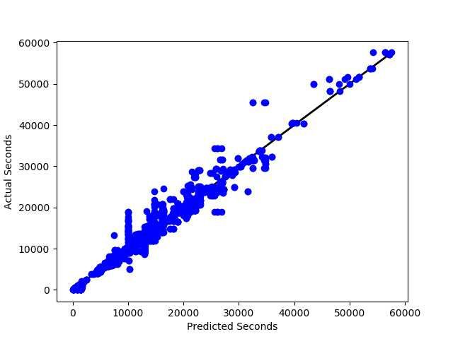
Director
                                                         Director
                                                                                                                         Friend
                                                       Martin Scorsese
                                                                                   *                Student                 ..          Recruiter
                                                                                                         Alex                .                Tim
                             Award                                       Student       Recruiter
              Award          Oscar                                                                              Friend            Colleague

                         Academy Award                                      Query Q2
                                                                                                    Student         Software Eng      HR Manager
                                                                                                         Bob            Adam                  Paul
                                                                                                                 Social Graph G2

     Brad              [Brad Pitt, Brad Dourif, ...]
            Query Q1                      Knowledge Graph G1
                             (a)                                                                   (b)

Fig. 1: Approximate graph querying, (a) Knowledge Search and (b) Social Search
match as illustrated in Fig. 1 (a). Each pattern node in Q1 may have a large
number of candidate matches.
    As shown in this example, graph queries, unlike their relational counterparts,
can be “approximate” or “structureless” [25], i.e. not well supported by rigid
algebra and syntax. The ambiguous keyword “Brad” in this example query can
lead to either “Brad Pitt”, “Brad Dourif”, or many other nodes in our data
graph. It is often hard to exploit algebra and operator-level features (e.g. number
of “join”) [1,8] for graph matching queries—and it is exceedingly much harder for
reachability queries. Furthermore, graph data is often noisy and heterogeneous.
Features from data graph alone may not be reliable for QPP tasks.
Example 2. Social search. Consider a business-oriented social network in which
nodes and edges represent people and their contacts, respectively. Suppose a
researcher wants to know how senior students can use their connections to con-
tact a recruiter and ask the recruiter to evaluate their resume. This question
can be represented as a regular path query from a student typed person to a
company recruiter. A regular path query Q2 as shown in Fig. 1(b) asks “which
recruiters are reachable from a student with at most 2 hops utilizing only friend
and colleague relations?” on the social network G2 . Note that each person might
have several positions at the same time and there might be restrictions on us-
ing connections. In this example, friend and colleague relations are allowed to
be used. Imposing other constraints on the number of connections to reach the
target person is also possible. The query node “Student” and “Recruiter” match
{“Alex”, “Bob”} and {“Tim”, “Paul”}, respectively.
    As illustrated in this example, while a common practice for QPP is to ex-
plore (logical and physical) query plans that are generated following a principled
manner [1], this is inapplicable for approximate graph queries. A regular path
may strict the edges we use to find the target which may change the query plan
dynamically during its computation. In addition, deriving statistics from the
graph data alone is expensive due to the sheer size of data, and the fact that the
underlying graph may change over time makes the process even more complex.
    In this paper, we present effective QPP methods for graph analytical
workloads over multiple metrics. We develop a learning framework that solely
makes use of computationally efficient query-oriented features and statistics
from executed graph queries, without imposing assumptions on query syntax
and algebra. Our goal is to build a general prediction framework for routinely
issued, structureless graph queries. We apply the framework to design a
workload optimization algorithm under bounded resources.
Contributions. Our main contributions are as follows:
– We propose a general learning framework (MGQPP) to predict multiple query
performance metrics for various graph analytical queries. The framework em-
ploys a novel training instance generation and multi-label regression models.
– We use the framework to develop performance prediction methods for
top-k queries [24], approximate matching queries [14], and general regular
expression-based reachability queries [5].
– We apply MGQPP to resource intensive querying, and develop learning-based
workload optimization strategies that make use of a Skyline Querying Algo-
rithm [21] over a “query table” and extract top-k resource-bounded queries
as a prioritized workload.
– We experimentally verify the efficacy of the proposed MGQPP framework
over real-world graphs.
Related Work. QPP has been studied extensively, especially in the informa-
tion retrieval community to either predict quality of answers [9] or resource
consumption [7, 19, 26]. Learning techniques for QPP have been applied in rela-
tional databases for SQL workloads [22] and in semi-structured data for SPARQL
queries [7, 8, 26]. Regression and Support Vector Machines were used to predict
the performance of SPARQL queries [7], where the features are collected from
SPARQL algebra and pattern [8]. A similarity metric was used to find if the
incoming query is similar to one of their training data and this similarity is used
as a part of their features [8]. The problem of SPARQL query execution time
prediction on RDF datasets has been considered by [26]. The authors of [26]
also used algebra and basic graph pattern features to train two support vector
regression and k-nearest neighbor models. In contrast to the mentioned query
languages, graph analytical queries are not well supported by algebra and apriori
query plans. These methods are not applicable to approximate graph querying.
Efficient processing of top-k queries is an essential requirement especially
when trying to manage very large data and multi access scenarios. Top-k pro-
cessing techniques in relational and XML databases are surveyed in [10].
Our framework differs from the related works discussed here in several ways.
(1) It considers performance as a multi-variant metric consisting of response
time, answer quality, and resource consumption. Thus, it uses a multi-label re-
gression model. (2) It does not assume any existing query plan or algebra. (3)
We obtain higher predction by introducing a diversified training instance gener-
ator using query templates of the available benchmarks [15]. (4) We study the
problem of multi-performance metric graph query workload optimization using
skyline algorithm which allows us to select the optimal subset of workload.
2 Problem Formulation
In this section, we formally define graph queries, performance metrics and the
prediction problem which will be used later in the proposed framework.2.1 Graph Queries
Data graphs. We consider a labeled and directed data graph G=(V, E, L),
with node set V and edge set E. Each node v ∈ V (edge e ∈ E) has a label
L(v) (L(e)) that specifies node (edge) information, and each edge represents a
relationship between two nodes. In practice, L may specify attributes, entity
types, and relation names [12].
Graph queries. A graph analytical query Q is a graph GQ = (VQ , EQ , LQ ).
Each query node u ∈ VQ has a label LQ (u) that describes the entities to be
searched for (e.g. type, attribute values), and an edge e ∈ EQ between two
query nodes specifies the relationship between the two entities. A match of Q in
G, denoted as φ(Q), is a subgraph of G that satisfies certain matching semantics,
induced by a matching relation φ. Specifically, each node u ∈ VQ has a set of
matches φ(u), and each edge e ∈ EQ has a set of matches φ(e) [17].
Next, we define the three query classes we study under this framework.
Top-k Subgraph queries [24]. A top-k subgraph query Q(G, k, L) defines the
match function φ as subgraph isomorphism, where the label similarity function
L is derived by a set of functions drawn from a library (e.g. acronym, synonym,
abbreviations), where each function maps nodes and edges (as ambiguous key-
words) in Q to their counterparts in G. A common practice to evaluate a top-k
subgraph query is to follow the Threshold Algorithm (TA) [4] that aggregates
top-k tuples in relational tables.
Approximate graph pattern matching [14]. A dual-simulation query Q(G, SV , θ)
relaxes the strict label equality to approximate matches of ambiguous keywords
as well as the subgraph isomorphism from 1-1 bijective mapping to matching
relations. The semantic has been used recently for event discovery [16, 18, 20].
Given a query Q = (VQ , EQ , LQ ) and a graph G = (V, E, L), a match relation
φ ⊆ VQ × V satisfies the following:
(1) for any node u ∈ VQ , there is a match v ∈ V such that (u, v) ∈ φ and
SV (u, v) > θ, where SV (·) is a similarity function over labels and θ is a threshold
which assures each node has an appropriate match in an answer [24].
(2) for any (u, v) ∈ φ and any child (resp. parent) of u (denoted as u0 ) in Q,
there is a child (resp. parent) of v (denoted as v 0 ) in G, such that (u0 , v 0 ) ∈ φ.
That is, it preserves both parent and child relationships between a node u and
its matches v.
Regular path queries [5]. Applications in traffic analysis, social analysis and Web
mining often rely on queries that carry a regular expression. Similar to [5], we
consider reachability queries as regular expressions.
A reachability query is defined as Qr = (s, t, fe , d, θ), where s and t are
predicates such as node types and labels, θ is a threshold for similarity function
SV (v, s) > θ (resp. SV (v, t) > θ) for accepting each node v, and fe is a regular
expression drawn from the subclass R ::= l | l≤d | RR. Here, l is any potential
relationship type of an edge or a wildcard , where the wildcard is a variable
standing for any L(e); d is a user-specified positive integer that determines the
maximum allowed hops from a source match s to a target match t. That is,
l≤d denotes the closure of l by at most d occurrences; and the operation of RRdenotes the concatenation of two regular expressions. The query finds all pairs
of source match vs and target match vt , where vs matches s and vt matches t
via φ, and there exists a path ρ from vs to vt with a label (concatenated edge
labels) that can be parsed by fe .
2.2 Performance Metrics
We focus on multi-metric QPP for graph analytical queries. We consider the
following metrics: (1) response time t(Q, G, A), the time needed by algorithm
A to return answers to query Q in graph G; (2) quality q(Q, G, A), the highest
quality score of the answers returned by A in G; and (3) memory m(Q, G, A),
the memory needed to answer Q by A in G. For simplicity, we use t, q and m
to denote the three metrics.
Response time and memory are rather familiar performance metrics. In con-
trast, the query answer quality metric is not straightforward. We next introduce
a generic quality function F (·) for graph analytical queries.
Generic quality function. Given a query Q and its match φ(Q), we consider
the following: (1) There is a node scoring function SV (u, φ(u)) that computes
a similarity score (normalized to be in (0, 1]) between a query node u and its
node matches φ(u) induced by φ(Q); and (2) similarly, there is an edge scoring
function SE that computes a score for each edge e in Q and its match φ(e).
A similarity function SV (·) should consider both semantic constraint LV (·)
and topological constraint TV (·). Each node match produces a similarity score
SV (·) = LV (·) ∗ TV (·) ∈ (0, 1]. In practice, LV (·) supports various kinds of
linguistic transformations such as synonym, abbreviation, and ontology e.g. “in-
structor” can be matched with “teacher” which allows a user to pose queries
without having sophisticated knowledge about the vocabulary or schema of the
graph [24]. Furthermore, query topological constraints such as node degrees are
taken into account by TV (·). Analogously, the similarity functions SE and TE
are defined over edge matching. When the similarity functions are common for
both nodes and edges, we do not write the subscript in the rest of the paper.
We consider a general quality function F (·) that aggregates the node and
edge matching scores to produce a matching score defined as:
P P
v∈VQ SV (v, φ(v)) + e∈EQ SE (e, φ(e))
F (Q, φ(Q)) = , (1)
N
where N is a normalizer to get the score in [0, 1]. By default, a normalizer can
be set to |G|, since |φ(Q)| ≤ |G|.
The quality of an answer depends on the query semantics. We will make use
of the general function F (·) as a component to specialize the quality metric q
for specific query classes.
Top-k search quality function. Given a graph query Q, an approximate answer
φ(Q), and an integer k, we define the quality function qtopk for top-k search as
follows: Pk
F (Q, φi (Q))
qtopk (Q, φ(Q), k) = i=1 (2)
kHere in its F (·) , we set topological similarity function T (·) = 1 since φ(Q)
is isomorphic to Q. Note that the value of qtopk lies in (0, 1] and is an average
of qualities over all answers retrieved by top-k querying. That is, the closer the
value is to 1, the more similar the labels of the matches are to that of the query.
Approximate pattern matching quality function. In the F (·) of this algorithm,
since φ(Q) in simulation might be a topological approximation of Q, to compare
the topology of the induced graph on φ(Q) to Q where the degrees of matches
and the number of matched edges can be higher or lower than query nodes and
deg(v) deg(VQ )
edges, respectively, we set TV (VQ ) = min( deg(V Q)
, deg(v) ) , where v ∈ φ(VQ )
and deg(v) (resp. deg(VQ )) is the degree of node match v (resp. query node
VQ ), in order to keep the quality metric in the range(0, 1]. Furthermore, we set
|EQ |
TE (·) = min( |E(φ(Q))|
|EQ | , |E(φ(Q))| ). The quality qSim is then defined as follows:
P
φ(Q) F (Q, φ(Q))
qSim (Q, φ(Q)) = , (3)
|φ(Q)|
where |φ(Q)| is the number of total matches retrieved by a simulation algorithm.
We remark that in addition to considering the linguistic similarity by L(·), topo-
logical constraints are also assessed by T (·) ∈ (0, 1], affecting the overall quality
of F (·). That is, the closer the structure of an answer is to the query, the closer
the quality is to 1.
Regular path quality function. Intuitively, the higher quality for reachability
queries happens when query node pair (s, t) exactly matches the answer pair
(φ(s), φ(t)) and also the length of shortest path between φ(s) and φ(t) is smaller
(fewer number of hops between φ(s) and φ(t)). Hence, given the data graph G
1
and graph query Q, we set SE = 0 and TV = |E(φ(Q)| . Therefore, the quality of
the retrieved answers is defined as follows:
P
φ(Q) F (Q, φ(Q))
qreach (Q, φ(Q)) = , (4)
|VQ ||φ(Q)|
where |φ(Q)| means the number of distinct pairs (φ(s), φ(t)) and |VQ | = 2 for
reachability queries.
2.3 Performance Prediction
In this subsection, our goal is to formulate QPP for graph analytical workloads.
We consider a mixed workload W={Q1 , . . . , Qn } over a set of query classes Q,
where each query Qi is an instance from a query class in Q, and the vector M,
the multi-metrics performance to be predicted. We instantiate M =< t, q, m >,
where t, q, and m are the response time, answers quality, and memory usage
as measure by the number of visited nodes, respectively. The problem of multi-
metric graph query performance prediction, denoted as MGQPP, is to learn a
prediction model P to predict the performance vector of each query instance in
W with maximum accuracy measured by a specific metric.
A metric must measure how well the performance of future queries is likely
to be predicted. We seek to minimize the error depending on the type of theDiversified
Fig. 2: Prediction framework for MGQPP
queries and the scale of their performance values. Therefore, we use R-Squared,
a widely used evaluation metric [8] to evaluate our framework. To empirically
verify the robustness of our models, wePalso consider mean absolute error (MAE)
n
besides R-Squared. MAE, defined as n1 i=1 |ŷ − y|, is an absolute comparison of
predictions and eventual outcomes [6].
GQPP as regression. We approach MGQPP as a regression problem. We use
the following construction:
Input: A data graph G, training workload WT
Output: a prediction model P to predict a set of performance metrics M that
maximizes the prediction accuracy of all metrics in the same time.
The problem is to learn, using a multi-label regression, a function f (x) = y
that maps a feature vector x of a query to a set of continuous values y corre-
sponding to the exact response time, quality of the retrieved answer and number
of visited nodes (as an indicator for memory usage) of the query.
3 The Framework
Our multi-metric graph query performance prediction framework is illustrated in
Fig. 2. Following statistical learning methodology, the framework derives a pre-
diction model based on training sets (learning) and predicts query performance
for test data points based on the derived model (prediction). Our goal is to adapt
the framework to accomplish mixed graph analytical workload prediction.
3.1 Learning Phase
Besides the effect of feature selection, model choice, and loss function definition
in any learning-based predictive frameworks, training data plays an important
role in ensuring that a model is comprehensive enough to predict a wide variety of
future inputs. Here, our training data is a set of queries, called training workload
WT . In order to generate a good, small yet representative training data, MGQPP
is armed with a diversified query generation module, which we describe below.Diversified query generation. Given a query class Q, a data graph G and
a standard evaluation algorithm A, the training workload WT is a set of pairs
−→ −→
(Qi , M(Qi )), where Qi refers to a feature representation of query Qi , and M(Qi )
is the actual performance metrics obtained by evaluating Qi with algorithm A.
An empirical study of over 3 million real-world SPARQL queries has shown
that most queries are simple and include few triples patterns and joins [2]. In-
deed, in order to simulate real-world queries, it is enough to generate small
queries by a bounded random walk on the data graph. However, while a naive
way of generating training queries is sampling the data graph using a random-
walk [13], it does not guarantee the diversification of the training instances to
provide additional information for the predictor. Hence, we adopt a batch mode
active learning [23] to generate diversified queries. Research has shown that an
intelligent selection of training data instances using active learning provides high
accuracy with much fewer instances compared to a blind selection strategy [23].
We formulate the query generation problem as follows. Given a data graph
G, a bound b on the size of the query, the number of training queries N , and a
dissimilarity threshold σ, select a set of queries such that the diversity d(Qi ) of
each query Qi compared to the current training set WT is greater than σ. Given
the query Qi generated at the step i, the diversity is defined as:
d(Qi ) = avg CosDis(Qi , Qj ), (5)
∀Qj ∈WT ;j σ. The algorithm
terminates when N queries are generated and added to the training workload.
Feature generation and learning prediction model. The learning frame-
work generates the training workload WT . In particular, it generates queries (as
discussed), evaluates the queries over the data graph G (stored and managed
by the knowledge base) by invoking standard query evaluation algorithms, and
collects the performance metrics and features for each query to construct WT .
The predictive model is then derived by solving the multi-variable regression
problem (details discussed in section 3.2).
Features. As remarked earlier, graph analytical queries, unlike their relational
counterparts, cannot be easily characterized by features from operators, alge-
bra, and apriori query plans. Features from data alone may also be unreliable.We hence consider four classes of query-oriented features. The classes are called Query, Sketch, Algorithm, and Quality features since they characterize statistics from query instances, accessed data, search behavior, and similarity values, re- spectively. Later in the paper, we will use the shorthands Q, S, A and L to refer these four features, respectively. (a) Query features encode the topological (e.g. query size, degree, cyclic) and semantic constraints (e.g. label, transformation functions [25]) from query terms. (b) Sketch features. The idea is to exploit statistics that estimate the specificity and ambiguity of a query by “sketching” the data that will be accessed by the queries. These features may include the size of candidates (the nodes having the same or similar labels to some pattern query nodes), degree of sampled candi- dates, and statistics of sampled neighborhood of the candidates. By paying an affordable amount of time, these features significantly contribute to the predic- tion accuracy of graph queries (as verified in [19]). (c) Algorithm features refer to the features that characterize the performance of graph querying algorithms. For example, top-k graph search typically decom- poses a query to sub-queries, and assembles the complete results by aggregating partial matches as multi-way joins [24]. We found that features such as the num- ber of decompositions and “joinable” candidates are very informative and critical to predict the cost of top-k search. (d) Quality features. MGQPP also uses statistical features that directly affect the quality of the retrieved results. Such features include minimum, average, and maximum similarity values between a query and the candidates. Since the similarity computation is expensive, to aid efficient features computation at the prediction time, we follow an approach in which a one-time process calculates the features for any pair of nodes (resp. edges) in G and stores them in memory. The proposed features can all be computed efficiently. Indeed, they can be extracted by fast linear scans and sampling over queries and data graphs, and are well supported by established database indexing techniques [24]. Feature analysis. We studied the contribution of features in the framework by calculating their importance. For space considerations, we omit a complete description of the importance analysis we performed to select the features we use for each query algorithm, and instead, we discuss them only at a high level here. Top-k subgraph queries. Algorithm and Sketch features were find to play the most important role in predicting the performance of top-k subgraph queries. Query features were found to be next in the importance ranking. Indeed, the perfor- mance of top-k subgraph queries may highly depend on the algorithm behavior (decomposition, n-way joins in the TA-style computation), which can be more critical than the number of joins (a plan-level feature) in a graph pattern [8]. Approx. pattern matching. Unlike top-k subgraph queries, we find Sketch fea- tures to be the most important for predicting the efficiency of the computation for dual-simulation queries. Next in importance for dual-simulation performance
prediction were candidate size and degrees. Query size, in contrast, was found
to be not as important.
Regular path queries. We found that quality of reachability queries is most de-
termined by “average similarity values of candidates”. Sketch features on source
and target candidates come second in rank and query feature hop bound d comes
third in rank. Indeed, the more candidates and more neighbors they have, and
the more hops a query needs to visit, the more chance a reachability query have
to find a match pair.

3.2   Prediction phase
We use a multi-label learning framework as our primary predictive model. A
multi-label or multi-output problem is a supervised learning problem with several
outputs (potentially with correlations) to predict. In our case, we also observed
that the output values related to the same input are themselves correlated.
Hence, a better way is to build a single model capable of predicting all outputs
at the same time. Such an approach will make the framework save training time,
reduce complexity, and increase accuracy.
    In order to build our multi-label model, we use XGBoost [3], an ensemble
method, as our inner predictive model. XGBoost trains each subsequent model
using residuals of current prediction and true values. Extensive studies have
shown that XGBoost outperforms other methods on regression problems since it
reduces the bias and variance at the same time. We note however that the GQPP
problem has been addressed suitably by random forest regression models in the
study [19].
    In the next step, the prediction model is applied to predict the performance
of new queries. Upon receiving a query workflow, the framework collects the
queries, computes the query features, and predicts the query performance metrics
vector. The predicted results can then be readily applied for resource allocation
and workload optimization (see Section 4). Note that the proposed MGQPP
framework can be specialized by “plugging in” other performance metrics to be
applied for other type of graph queries.

4     Workload Optimization
We use resource bounded workload optimization as a practical application to
illustrate one of the utilities of our MGQPP framework. We consider a mixed
query workload W={Q1 , . . . , Qn } over a set of query classes Q, where each
query Qi is an instance of a query class in Q and is associated with a profit pi .
After execution of the query Qi , a set of performance metrics Mi is associated
with Qi . Now using MGQPP, we can associate a predicted performance metrics
M̂i to each query before its execution.
Resource-bounded query selection. We formalize the multi-metric workload
optimization problem as the most profitable dominating skyline query selection
problem. In a multi-dimensional dataset, a skyline contains the points that are
not dominated by other points in any of the dimensions. A point dominates
another point if it is as good or better in all dimensions and better in at least
one dimension [11]. Using a modified version of a progressive skyline computation
strategy, we propose an algorithm with performance guarantee.
Given workload W, integer k to retrieve top queries, a set of predicted per-
formance metrics M̂, and resource bound C = {c1 . . . cm } corresponding to
the performance metrics M, the problem is to P find the most profitable dom-
n
inating skyline queries W 0 ⊆ W that maximize j=1 pj xj , xj ∈ {0, 1}, where
j =P {1, . . . , n} subject to the following two conditions.
n
1) j=1 wij xj ≤ ci , i = 1, . . . , m where each query Qj consumes an amount
wij > 0 from each resource i (e.g. time, memory, 1-quality). The binary decision
variables xj indicate which queries are selected.
2) Each query Qj ∈ W 0 is a skyline in W or by removing one or more queries in
W 0 , Qj becomes a skyline in the updated W.
Progressive skyline query selection. A skyline operator returns every query
not dominated by any one of the rest of the queries in any of the performance
metrics. Skyline operators have been found to be an important and popular
technique in multidimensional environments for finding interesting and repre-
sentative results. In practice, however, in order to solve the resource intensive
workload optimization problem, the domination constraint may be too restric-
tive to take the resource budget into account. In addition, profit maximization
can be considered as an independent metric to be optimized since it is not an
internal property of the query. Thus, we adapt progressive constrained skyline
computation in order to guarantee selection of both resourced bounded and
most profitable queries among the ones that are not dominated by the rest.
Our algorithm, denoted as skySel, is outlined in Fig. 3. The algorithm uses a
priority queue L sorted in a decreasing order by profit (of queries). The queue L
contains the queries that are not dominated by the rest of queries in W at any
time. The algorithm skySel starts with an empty set of W 0 and uses a skyline
operator S that progressively returns skyline queries (line 1-2). It then populates
the queue L with the first set of skyline queries (line 3). While the queue is not
empty, there exists an available resource on all dimensions, and not enough
queries are selected, it iteratively retrieves the most profitable non-dominated
query Qi from L (line 5), removes Qi from the initial workload W, updates the
set of skyline queries in L with new queries and available resource vector C, and
adds Qi to the set of selected queries (line 6-8). When the algorithm terminates,
W 0 is returned as the optimized query workload.
Correctness & Complexity. The algorithm skySel maintains two invariant at the
beginning of each iteration: I1 ) the queries in L are not dominated by queries in
the current W ∪L; and I2 ) the most profitable query in the set of non-dominated
queries is selected as the top element in L. The correctness of I1 follows from the
correctness of skyline computation and the correctness of I2 follows from priority
queue operations. Thus, the algorithm correctly finds the most profitable non-
dominated queries.
A simple implementation of skyline takes O(nlogn) to find the skyline
queries [11]. The skyline operation is computed at most n times. Thus the overall
complexity of algorithm skySel is O(n2 logn).Algorithm skySel
Input: query workload W = {hQ0 , M̂0 , p0 i, . . .}, integer k
resource bound C = {c1 . . . cm }.
Output: selected queries W 0 .
1. set W 0 ← ∅; let S be a skyline operator;
/* L in a decreasing order by profit pi */
2. let L be a priority queue;
3. L ← L ∪ S.nextSkylineQueries(W);
4. while |W 0 | < k and C has enough resource and L 6= ∅
/* get the most profitable non-dominated query */
5. query Qi ← L.pull();
6. W.remove(Qi );
7. L ← L ∪ S.nextSkylineQueries(W);
8. W 0 ← W 0 ∪ Qi ; C ← C − M̂i ;
9. return W 0 ;
Fig. 3: skySel: Multi-metric Query Workload Optimization Algorithm
5 Experimental Evaluation
Using two real-world graphs, we conduct three sets of experiments to evaluate the
following: (1) Performance of MGQPP over different metrics and a comparison
to baselines; (2) Impact of diversified query workload generation vs. random
generation on the accuracy of the predictors; and (3) Effectiveness of workload
optimization using a case study.
Experimental setting. We used the following setting.
Datasets. For the experiments, we use Pokec and DBpedia, two real-world graphs.
Pokec1 is a popular online social network in Slovakia. It has 1.6M users with
34 labels (e.g. region, language, hair color, etc.) and 30M edges among users.
DBpedia2 is a knowledge graph, consisting of 4.86M labeled entities (where each
label is one of 1K labels such as “Place”, “Person”) and 15M edges.
Workload. We develop two query generators, a random generator using a
random-walk with restart and a diversified query generator (see Section 3.1).
We instantiate each generator for both graph pattern queries and reachability
queries to construct training and test data sets over the two real-world networks.
Graph pattern queries. To generate graph pattern queries, we use the DBPSB
benchmark [15], a DBpedia query benchmark. To achieve this, we use DBPSB
query templates, and subsequently use the query topology to build an unlabeled
graph. The graph is then assigned a type sampled from the top 20% most fre-
quent types in the ontologies of Pokec and DBpedia. Furthermore, we set the
maximum size of queries b = 6 (i.e. max |EQ | = 6) as it has been observed that
most of the real-world SPARQL queries are small [2]. Although this process of
query generation is a common practice [24], since we use these queries as a train-
ing data, it is important to consider the effect of each sample to the learning
phase of the model. To address this, we employ the proposed diversified training
1
https://snap.stanford.edu/data/soc-pokec.html
2
http://wiki.dbpedia.org/query generation to make sure that the generated training data is informative
to our learning model. (Details of the algorithm discussed in Section 3.1).
We draw the matching function L(·) from a library of similarity functions as
in [25]. We then set an integer k drawn from [10, 100].
Reachability queries. For reachability queries Q(s, t, d, G), we set d ∈ [1, 4], and
randomly select a pair of labels, from the top 20% most frequent labels in G.
We sampled 4K queries, 1K for each d.
Algorithms. We implemented the following, all in Java.
(1) Standard query evaluation algorithms (Sec. 3), including:
– STAR, the algorithm of [24] for top-k subgraph queries,
– dual-simulation [14], for dual-sim queries, and
– a variant of Breath-First Search, for reachability queries.
(2) Query workload optimization algorithms for top-k most profitable dominat-
ing queries, including
– a progressive skyline computation algorithm (skySel) and
– Rndk , a baseline algorithm that randomly selects k queries to be executed in
the workload.
Predictive model. We implemented the XGBoost model as our predictive model
by leveraging the scikit-learn3 library and APIs.
Metrics. We use two metrics as remarked in Section 2: R-Squared and MAE.
Test platform. We ran all of our experiments on a Linux machine powered by an
Intel 2.30 GHz CPU with 64 GB of memory. Each test is repeated 5 times and
the averaged results are reported.
Result overview. Here is a summary of our findings. Using the four classes of
features and the XGBoost predictive model, we show the performance of analyti-
cal graph queries can be predicted quite accurately (Exp-1). Diversified training
workload enables constructing a general model (Exp-2). Our case study veri-
fies the effectiveness of our approach for query workload management (Exp-3).
Furthermore, we found that using well-supported graph neighborhood and label
indices [25], it takes on average 15.3 seconds to predict the performance of a
workload of 433 queries, with total response time of 15 minutes. We next discuss
our findings in details.
Exp-1: Performance of MGQPP. We estimate the accuracy of the XGBoost
model using l-fold cross-validation [1]. We set l = 5.
Top-k Dual-Simulation Reachability
DBPedia Pokec DBPedia Pokec DBPedia Pokec
Time 0.819 0.985 0.818 0.926 0.928 0.869
Quality 0.978 0.991 0.827 0.906 0.973 0.985
Memory 0.981 0.998 0.995 0.995 0.938 0.993
Table 1: Performance evaluation measured in R2
Table 1 lists the R-Squared accuracy of XGBoost for the three query classes
and the performance metrics response time, quality, and memory for both of
3
http://scikit-learn.orgthe data sets Pokec and DBpedia. Over all datasets and performance metrics, we
found that XGBoost attains an accuracy ranging between 61.64% and 99.84%. In
addition, we found that the framework yields MAE of 420 milliseconds on time,
less than 0.0008 percent on quality, and 279.4 nodes on predicting the number
of visited nodes as an indicator of memory usage in querying.
Actual vs. predicted. Fig 4.a shows a comparison between predicted and actual
values of the XGBoost model for top-k subgraph query and the performance metric
time for 1K queries. Fig 4.b shows similar comparison for dual simulation query
and performance metric quality, and Fig 4.c for reachability query and metric
memory. In each of the cases, the results for the remaining two performance
metrics are similar and are omitted for space considerations.
0.6 0.6 0.7 0.75 0.8 0.8 0.9 0.95 0.99
60000
6
6
nodes)
60000
0.98
nodes)
50000
5
5
0.95
Actual (Seconds)
50000
visited nodes)
visited nodes)
0.90
of(# of10K
40000
4
4
(# of10K
40000
0.85
Actual
30000
3
3
30000
of
0.80
Act ual
Act ual
Actual (#
Actual (#
0.75 20000
2
2
20000
0.70
10000
1
1
10000
0.65
0
0
0 0
0.60
0.60
0.6 0.65
0.65 0.7 20000
100000.70 0.75 0.80
0.75 0.8 0.85 0.8540000 0.90
0.9 50000
0.95
0.95 0.99
0.98
0 1 2 3 4 5 6 0 30000 60000 00 10000
1 20000
2 30000
3 40000
4 50000
5 60000
6
Predicted (Seconds) Predicted (# of 10K nodes)
Predict Predicted
ed (# of visited nodes)
Predicted (# of 10K nodes)
Predict ed (# of visited nodes)
(a) Top-k; Time (b) DualSim; Quality (c) Reachability; Memory
Fig. 4: Actual vs. Predicted values for different algorithms and metrics
Comparison with related works. As we mentioned in section 1 related work, most
of the related papers use SPARQL for querying semi-structured data. In fact, [19]
is the first attempt that addressed the QPP in the context of general graph
queries, although only on execution time. Anyhow, recent SPARQL query per-
formance prediction approaches [7, 26] used also DBPSB templates to generate
queries and DBpedia as the underlying graph. Thus, we compare our results with
their results (as reported in [7, 26]) using the same metric denoted as “relative
error” in Table 2. The results shows that our general framework outperforms
recent QPP approaches [7, 26] in both accuracy and efficiency of training time.
Model Features Relative Err 1K Q’s Train (sec)
[7] X-means+SVM+SVR Algebra+GED 14.39% 1548.45
[26] SVM+Weighted KNN Algebra+BGP+Hybrid 9.81% 51.36
Ours Multi-label XGBoost Q+A+S+L 6.91% 35.33
Table 2: Performance comparison with the related works
Exp-2: Diversified queries vs. random generation. Table 3 shows the ac-
curacy of prediction using our diversified query generator compared with that
of a simple random generation used as a baseline. It can be seen that diversified
query generation outperforms the baseline by large margins consistently over all
performance metrics.
Exp-3: Query workload optimization. We next conduct a case study to test
the effectiveness of MGQPP for query workload optimization. The workloads are
simulated as follows. (1) We generate a workload of 1K queries for each of the
three query classes top-k subgraph, dual-sim, and reachability. (2) The queriesTest
Time Quality Memory
Rnd Dvs Rnd Dvs Rnd Dvs
Rnd 40.59 25.78 74.51 66.83 62.06 36.2
Train
Dvs 70.41 89.68 78.46 91.44 82.37 90.84
Table 3: Diversified (Dvs) vs. Random (Rnd) query generation accuracy (%)
are sent to each optimizer in batch. Given user input, the optimizer selects
queries to be executed.
RndK RndK RndK
SkySel SkySel SkySel
1.0 1.0
0.9
0.4 0.8
1 - Quality
0.8
1 - Quality
1 - Quality
0.3 0.7
0.6 0.6
0.2 0.5
0.1
0.4 0.4
0.0 0.2 0.3
0.2
0.0
Me 15.0
20
Mem6 5 1518) Me 400300 14
mo 12.5
ry( 10.07.5
15 ds)
10 econ ory(#4 3 1012onds mo 1012ds)
5 8e (Sec
ry( 200
#K M of 2 #K 6 8Secon
of n 5.02.5 5 me (S node1 0 2 of n 100 4 (
ode 0.0
s)
0 Ti s) 0 Tim ode 0
s)
0 2 Tim
e
(a) Top-k (b) Dual-Simulation (c) Reachability
Fig. 5: Actual performance of selected queries, - skySel vs. Rndk over DBpedia
Given workload W and k = 10, we invoke skySel to select k most profitable
dominating queries and Rndk as a random strategy. Fig. 5(a), 5(b), and 5(c)
demonstrate the selected queries by skySel and Rndk for top-k, dual-sim, and
reachability, respectively. The size of points shown in the figures are proportional
to their profit. The closer the points are to the origin of coordinate system and
the larger their size is, the better. The figures tell us that skySel outperforms
Rndk by selecting non-dominated queries with more profits. In addition, the
results show that the query profit utilization of skySel algorithm is 54% more in
comparison to Rndk scenario on average of 10 different workloads.
6 Conclusion
We have presented a learning-based framework to predict performance of graph
queries in terms of their response time, answer quality, and resource consump-
tion. We introduced learning methods for both graph pattern queries, defined
by subgraph isomorphism, dual-simulation, and reachability queries. We showed
that by exploiting computationally efficient features from queries, sketches of
the data to be accessed, and algorithm itself, multi-metric query performance
can be accurately predicted using the proposed multi-label regression model. We
also introduced a workload optimization strategy for selecting top-k best queries
to be executed that maximizes the quality and minimizes the time and mem-
ory consumption. Our experimental study over real-world social networks and
knowledge bases verifies the effectiveness of the learned predictors as well as the
workload optimization strategy.
7 Acknowledgments
Sasani and Gebremedhin are supported in part by NSF CAREER award IIS-
1553528. Namaki and Wu are supported in part by NSF IIS-1633629 and Huawei
Innovation Research Program (HIRP).References
1. Akdere, M., Çetintemel, U., Riondato, M., Upfal, E., Zdonik, S.B.: Learning-based
query performance modeling and prediction. In: ICDE. pp. 390–401 (2012)
2. Arias, M., Fernández, J.D., Martı́nez-Prieto, M.A., de la Fuente, P.: An empirical
study of real-world sparql queries. arXiv preprint arXiv:1103.5043 (2011)
3. Chen, T., Guestrin, C.: Xgboost: A scalable tree boosting system. In: KDD. pp.
785–794 (2016)
4. Fagin, R., Lotem, A., Naor, M.: Optimal aggregation algorithms for middleware.
Journal of computer and system sciences 66(4), 614–656 (2003)
5. Fan, W., Li, J., Ma, S., Tang, N., Wu, Y.: Adding regular expressions to graph
reachability and pattern queries. In: ICDE. pp. 39–50 (2011)
6. Guo, Q., White, R.W., Dumais, S.T., Wang, J., Anderson, B.: Predicting query
performance using query, result, and user interaction features. In: RIAO (2010)
7. Hasan, R.: Predicting sparql query performance and explaining linked data. In:
European Semantic Web Conference. pp. 795–805 (2014)
8. Hasan, R., Gandon, F.: A machine learning approach to sparql query performance
prediction. In: WI-IAT (2014)
9. Hauff, C., Hiemstra, D., de Jong, F.: A survey of pre-retrieval query performance
predictors. In: Proceedings of the 17th ACM conference on Information and knowl-
edge management. pp. 1419–1420. ACM (2008)
10. Ilyas, I.F., Beskales, G., Soliman, M.A.: A survey of top-k query processing tech-
niques in relational database systems. CSUR p. 11 (2008)
11. Kossmann, D., Ramsak, F., Rost, S.: Shooting stars in the sky: An online algorithm
for skyline queries. In: VLDB. pp. 275–286 (2002)
12. Lu, J., Lin, C., Wang, W., Li, C., Wang, H.: String similarity measures and joins
with synonyms. In: SIGMOD (2013)
13. Lu, X., Bressan, S.: Sampling connected induced subgraphs uniformly at random.
In: SSDBM. pp. 195–212 (2012)
14. Ma, S., Cao, Y., Fan, W., Huai, J., Wo, T.: Capturing topology in graph pattern
matching. VLDB pp. 310–321 (2011)
15. Morsey, M., Lehmann, J., Auer, S., Ngomo, A.C.N.: Dbpedia sparql benchmark –
performance assessment with real queries on real data. In: ISWC (2011)
16. Namaki, M.H., Lin, P., Wu, Y.: Event pattern discovery by keywords in graph
streams. In: IEEE Big Data (2017)
17. Namaki, M.H., Chowdhury, R.R., Islam, M.R., Doppa, J.R., Wu, Y.: Learning to
speed up query planning in graph databases. In: ICAPS (2017)
18. Namaki, M.H., Sasani, K., Wu, Y., Ge, T.: Beams: bounded event detection in
graph streams. In: ICDE. pp. 1387–1388 (2017)
19. Namaki, M.H., Sasani, K., Wu, Y., Gebremedhin, A.H.: Performance prediction
for graph queries. In: NDA (2017)
20. Namaki, M.H., Wu, Y., Song, Q., Lin, P., Ge, T.: Discovering graph temporal
association rules. In: CIKM. pp. 1697–1706 (2017)
21. Papadias, D., Tao, Y., Fu, G., Seeger, B.: Progressive skyline computation in
database systems. TODS pp. 41–82 (2005)
22. Wu, W., Chi, Y., Zhu, S., Tatemura, J., Hacigümüs, H., Naughton, J.F.: Predicting
query execution time: Are optimizer cost models really unusable? In: ICDE. pp.
1081–1092 (2013)
23. Xu, Z., Hogan, C., Bauer, R.: Greedy is not enough: An efficient batch mode active
learning algorithm. In: ICDMW. pp. 326–331 (2009)
24. Yang, S., Han, F., Wu, Y., Yan, X.: Fast top-k search in knowledge graphs. In:
ICDE (2016)
25. Yang, S., Wu, Y., Sun, H., Yan, X.: Schemaless and structureless graph querying.
VLDB (2014)
26. Zhang, W.E., Sheng, Q.Z., Taylor, K., Qin, Y., Yao, L.: Learning-based sparql
query performance prediction. In: International Conference on Web Information
Systems Engineering. pp. 313–327 (2016)You can also read