Predicting Food Security Outcomes Using CNNs for Satellite Tasking
←
→
Page content transcription
If your browser does not render page correctly, please read the page content below
Predicting Food Security Outcomes Using CNNs for Satellite Tasking

                                                                              Swetava Ganguli, Jared Dunnmon, Darren Hau
                                                                        Department of Computer Science, 353 Serra Mall, Stanford, CA 94305
                                                                                   {swetava, jdunnmon, dhau}@cs.stanford.edu
arXiv:1902.05433v2 [cs.CV] 25 Apr 2019

                                                                     Abstract                                  Over the last several years, an increasing supply of satel-
                                                                                                            lite data has enabled a variety of important studies in ar-
                                              Obtaining reliable data describing local Food Security        eas of environmental health, economics, and others (Safyan
                                              Metrics (FSM) at a granularity that is informative to
                                                                                                            2015). The unique insight attainable from such datasets has
                                              policy-makers requires expensive and logistically dif-
                                              ficult surveys, particularly in the developing world. We      continued to be integrated into the intelligence operations
                                              train a CNN on publicly available satellite data describ-     of both public and private sector entities to the point that a
                                              ing land cover classification and use both transfer learn-    number of modern processes would not be possible in their
                                              ing and direct training to build a model for FSM predic-      absence (Meyer 2014). Additionally, the increasingly com-
                                              tion purely from satellite imagery data. We then propose      mon integration of hyperspectral sensors into commercial
                                              efficient tasking algorithms for high resolution satel-       satellite payloads has extended the types of conclusions that
                                              lite assets via transfer learning, Markovian search algo-     can be drawn from satellite imagery alone (Romero, Gatta,
                                              rithms, and Bayesian networks.                                and Camps-Valls 2014). Recent developments deep CNNs
                                                                                                            have greatly advanced the performance of visual recogni-
                                                    Introduction and Background                             tion systems. In addition, using convolutional neural net-
                                                                                                            works and GANs on geospatial data in unsupervised or
                                         In a recent paper (Neal Jean 2016), Convolutional Neu-             semi-supervised settings has also been of interest recently;
                                         ral Networks (CNNs) were trained to identify image fea-            especially in domains such as food security, cybersecurity,
                                         tures that explain up to 75% of the variation in local level       satellite tasking, etc. ((Ganguli, Garzon, and Glaser 2019),
                                         economic outcomes. This ability potentially enables policy-        (Dunnmon et al. 2019), (Perez et al. 2019)). In this pa-
                                         makers to measure need and impact without requiring the            per, we demonstrate the use of CNNs for predicting food
                                         use of expensive and logistically difficult local surveys          security metrics in poor countries in Africa using a com-
                                         ((United Nations 2014), (World Bank 2015), (Devarajan              bination of publicly available satellite imagery data from
                                         2013) and (Jerven 2013)). This ability is promising for some       the work of (Saikat Basu 2015) (“DeepSat” dataset) and
                                         African countries, where data gaps may be exacerbated by           UN data made available by the Stanford Sustainability Lab
                                         poor infrastructure and inadequate government resourcing.          (“SustLab” dataset).1 We also demonstrate the use of these
                                         According to World Bank data, during the years 2000 to             prediction models for tasking of relatively expensive, high-
                                         2010, 39 of 59 African countries conducted fewer than two          resolution satellites in a manner that maximizes the amount
                                         surveys from which nationally representative poverty mea-          of imagery collected over food insecure areas. The task con-
                                         sures could be constructed. Of these countries, 14 conducted       sidered in this paper is that of reaching the region of lowest
                                         no such surveys during this period (World Bank 2015). Clos-        food security while traversing a path that is globally optimal
                                         ing these data gaps with more frequent household surveys is        in the sense that the most food-insecure regions possible are
                                         likely to be both prohibitively costly, perhaps costing hun-       traversed.
                                         dreds of billions of U.S. dollars to measure every target of          Our project thus consists of two main challenges: (i) de-
                                         the United Nations Sustainable Development Goals in ev-            signing a CNN that ingests satellite images as an input and
                                         ery country over a 15-year period ((Jerven 2014)) and in-          outputs successful predictions of key food security met-
                                         stitutionally difficult, as some governments see little bene-      rics such as z-scores of stunting or wasting, and (ii) us-
                                         fit in having their lackluster performance documented ((De-        ing the food security predictions as rewards in a reinforce-
                                         varajan 2013), (Sandefur 2015)). A popular recent approach         ment learning process to train a satellite to automatically tra-
                                         leverages passively collected data like satellite images of lu-    verse areas of interest. The first task is a machine-learning-
                                         minosity at night (nightlights) to estimate economic activity      intensive task which requires using a large dataset of images
                                         ((Henderson, Storeygard, and Weil 2011), (Chen and Nord-           to train a CNN model. We first utilize a publicly available
                                         haus 2011), (Pinkovskiy 2017)).
                                                                                                               1
                                         Copyright c 2019, Association for the Advancement of Artificial         Note that the DeepSat dataset is available online while the
                                         Intelligence (www.aaai.org). All rights reserved.                  SustLab dataset is currently proprietary.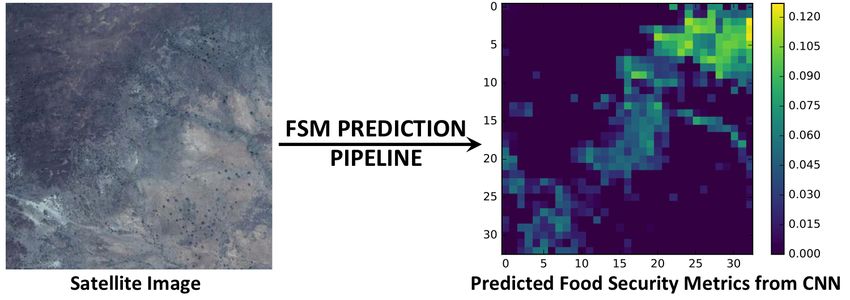
linked problems are described in the section titled “Auto-
mated Satellite Tasking for Food Security Measurements”.
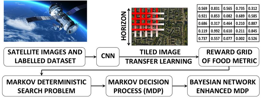
A full diagram describing the setup of this problem can be
found in Fig. 1.
Predicting Food Security Metrics with CNNs
Approach
Our first task is to effectively predict an FSM of interest di-
rectly from satellite data using a CNN. There exist multiple
Figure 1: A schematic describing the methodology for train- potential mechanisms by which to approach this problem,
ing CNN model which acts as an input for the path search and we perform this task with the aim both of generating a
algorithms reward grid for satellite tasking as well as obtaining useful
classification performance. The first approach, which repre-
sents our baseline, entails using the pre-trained network of
labeled dataset of 28 x 28 image tiles at 1m resolution la- (Jean et al. 2016) to extract features directly from the Sust-
beled with one of six ground cover classifications to train Lab images and predict the relevant food security metric.
a CNN focused on making predictions from overhead im- This network used a model originally trained on ImageNet
agery (Saikat Basu 2015). This trained network can be used to predict nighttime light levels from satellite imagery af-
to extract features from satellite imagery, which can in turn ter transfer learning to fine-tune coefficients. Features were
be used as the input to a ridge regression procedure aimed extracted using this network and food security data was pre-
at accurately predicting food security metrics. Alternatively, dicted from these features via ridge regression. The output
we can also use both direct learning and transfer learning was transformed to a ”classification” output by discretely
to enable direct prediction of food security metrics from a binning the stunting percentage (percentage height-for-age
pure CNN model, which will represent an interesting com- Z-scores below two standard deviations of the reference
parison to the regression procedure. We choose to use con- population) in bins of 0, 0−0.1, 0.1−0.2, 0.2−0.3, 0.3−0.4,
volutional neural networks for this task due to their superior and ≥ 0.4, which yielded a reasonably Gaussian distribution
performance on image classification problems. Their perfor- of the training data to the different bins. A ”classification ac-
mance generally results from effective integration of spatial curacy” could then be easily determined by comparing the
locality in convolutional features that aids accurate classi- predicted bin for each example to the bin in which its ground
fication predictions (Alex Krizhevsky 2012). We use a rela- truth value fell. Using this metric, the baseline attains a clas-
tively simple VGG-style architecture in this work (Karen Si- sification accuracy of 39 %.
monyan 2014). We attempt several different approaches to improving this
The second task is using the output FSMs to define the baseline prediction. First, we hypothesize that using a net-
state space for a set of path search algorithms. The general work pretrained on aerial imagery would yield features more
task of training a model to change the orientation of a useful in predicting food security metrics from satellite im-
satellite can be modeled as the problem of an agent finding agery than a network originally trained on ImageNet, which
its way to a high terminal reward on a grid via a Markovian describes optical images of a variety of different objects with
optimal path. For brevity, we will chose demonstrative features very different than those observed in satellite im-
numbers for easier explanation. Consider a very large image ages. We therefore utilize the publicly available DeepSat-6
(e.g. 400 x 400 pixel image showing a 1000 X 1000 km dataset of (Saikat Basu 2015) as an initial dataset, which
area). Let us call our trained CNN H. We train the CNN consists of 405,000 28 x 28 x 4 images (at 1m resolution)
on a dataset of 28 x 28 images (corresponding to 28 m x labeled with one of six ground cover classifications: barren,
28 m areas) and regress on a dataset of values of a given grassland, trees, road, building, and water. In order to enable
poverty/food security metric so that when an image is transfer learning, it is optimal that the resolution of the two
provided to the trained network, the output is a number datasets match – thus, we downsample the 1m DeepSat im-
quantifying this metric. More precisely: agery to an effective resolution of 2.4m to match that of the
SustLab data.
28 x 28 Resolution Image =⇒ H[Image] =⇒ A Once good classification performance on this DeepSat
number corresponding to food security metric. dataset was observed, we performed a tiling operation very
similar to that of (Saikat Basu 2015) on the SustLab data,
We can then tile the large 400 x 400 image into 332 12 where we resized each 400 x 400 image to 420 x 420 and
x 12 tiles, which are then upsampled to 28 x 28 to match then extracted 1089 12 x 12 tiles covering the full field of
the resolution of the original training set. For each tile, we view, which were then upsampled to 28 x 28 x 3 to align with
use our model to generate an associated food security metric the dimensions of the DeepSat data. Note that because the
which is treated as that tile’s reward in a search problem. SustLab data did not include a fourth near-IR channel (only
Given this setup, we will sequentially tackle three linked RGB), the near-IR channel was dropped from this analysis.
sub-problems that each add a layer of complexity and un- This tiling procedure results in a dataset in excess of 500,000
certainty to solve the complete problem. These sequentially image tiles, where each tile is labeled with the discrete bin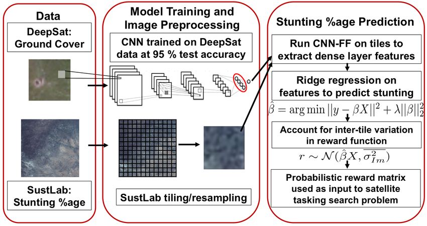
commensurate with the stunting percentage value of the full
image from which it was taken. This tiled dataset can be used
in three different ways: 1) direct learning, where we attempt
to learn the image label directly from the tiles, 2) transfer
initialization learning, where we perform a similar task, but
initialize the network weights with those learned from train-
ing on the DeepSat classification task, or 3) transfer learning
by directly using the DeepSat-trained model to extract fea-
tures from SustLab tiles, then using ridge regression to com-
pute a prediction of stunting percentage from these features.
   While it is possible to treat this as a regression problem,
we have chosen to treat it as a classification problem due
to the following considerations. First, the data from which
FSMs are drawn is survey data taken at a number of house-
holds within a given geographic area, the latitude and lon-
gitude of which are then correlated with those of the corre-
sponding satellite image. This data is fundamentally noisy in
nature, and it is less important that an exact value be recov-
ered than that the general state of food security in these ar-
eas be accurately reflected. Thus, a classification framework
seems appropriate, since binning the continuous results into
discrete classes eliminates some of this noise. Second, the r2
metric characteristic of a regression heavily penalizes large
single errors, whereas in this task, it is far more important to
accurately classify an areas as ”food secure” or ”food inse-         Figure 2: Computational graph for VGG-style network.
cure” than to be exactly correct about its stunting percentage
value, and the differential practical cost of large errors and
small errors in stunting percentage for single observations is     tory, which contains several thousand lines of code. For ex-
negligible.                                                        ample, ”layer utils.py” contains various layer types
                                                                   (i.e. general conv2d, batch normalization, maxpool), and
Infrastructure                                                     several initialization functions (Xavier, He) incorporated
                                                                   from recent literature. Model testing and training scripts can
To enable the studies described above, we created a
                                                                   be found in ”./transfer learning,” which utilize the
custom codebase from scratch, which handles all as-
                                                                   utilities in a modular fashion. Further, Google TensorBoard
pects of the above approach including data extract-
                                                                   functionality is integrated into the underlying training rou-
transform-load (ETL), CNN training/testing, and ridge re-
                                                                   tines in a way that enables direct visualization of training
gression/classification computation. Note that all code can
                                                                   curves, gradient flows, network activations, and the com-
be found in the repository
                                                                   putational graph. A computational graph for the VGG-style
ETL Data for the food security task is drawn from                  network used here for DeepSat classification can be found in
satellite images labeled with FSMs drawn from United               Fig. 2. Further, completed notebooks for training, monitor-
Nations Demographic and Health Surveys (DHS). Data                 ing, and performance of ridge regression can be found in the
is loaded from a set of .npy files describing the food             ”./notebooks” folder in the provided code repository.
security metrics of a target set of household surveys,
and the location (in terms of latitude and longitude) is           Results and Discussion
extracted from each location. These metrics are applied to
                                                                   DeepSat Land Cover Classification Task Before per-
a square of 0.09 in lat-lon coordinate length centered on
                                                                   forming the FSM prediction task, we first want to ensure
each reported survey location. Next, for each image in the
                                                                   that we have a viable network for land cover classification
dataset for Nigeria, which we focus on here, we assign it
                                                                   from which to perform transfer learning. To accomplish this
to the cluster in which its location is contained. All of this
                                                                   task, we have implemented a neural net architecture in the
is accomplished in the create clust dict2.py
                                                                   style of the classic VGGNet in TensorFlow, where the ma-
file in ./test in the code directory. Next, in
                                                                   jority of layers are either 3 x 3 convolutional layers or 2
./test/create test train set.py a number
                                                                   x 2 max pooling layers (Karen Simonyan 2014). Using a
of different options can be specified for creating test/train
                                                                   GPU-powered environment allows us to substantially de-
sets. In our case, we tile one image from each survey cluster
                                                                   crease training time (by over an order of magnitude) using
into 12 x 12 squares (afterwards upsampled to 28 x 28) and
                                                                   an NVIDIA Titan X GPU as opposed to the CPU environ-
populate the train/test sets with an 80/20 split of tiles from
                                                                   ment to which we were previously confined. Our first pass
each image.
                                                                   at training a viable network was performed on the Deepsat
Training and Monitoring Utilities to create, train, and            image set, with an architecture as described in Table 1:
monitor the network can be found in the ”./utils” direc-              Note that in Table 1, ”Lrn” refers to local response nor-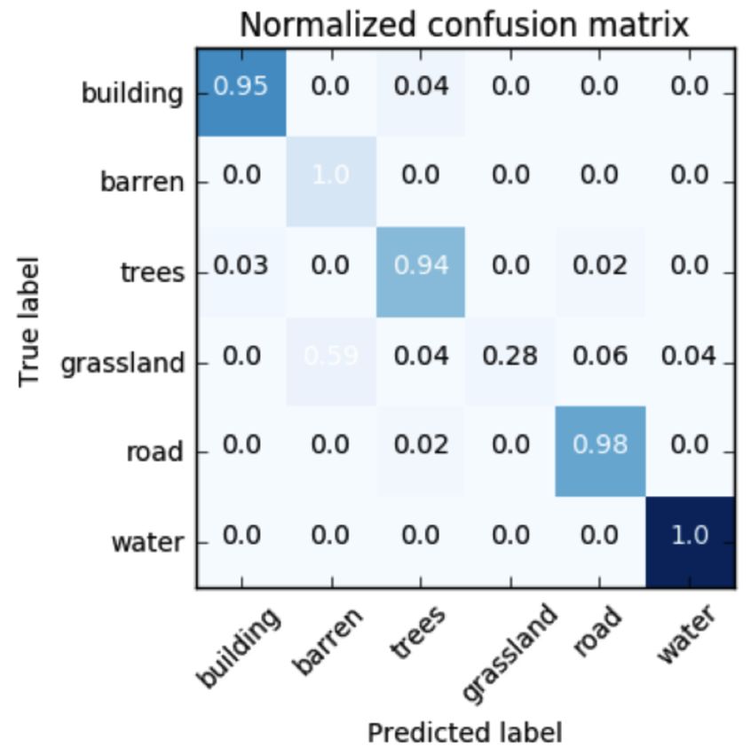
Table 1: Layout of VGG-Style Net Implementation.
          Layer         Type        Parameters
             0          Input      4 x 28 x 28
             1     Conv-Relu-Lrn    96 x 3 x 3
             2     Conv-Relu-Lrn    96 x 3 x 3
             3     Conv-Relu-Lrn    96 x 3 x 3
             4    Maxpool (2 x 2)        -
             5     Conv-Relu-Lrn    32 x 3 x 3
             6     Conv-Relu-Lrn    32 x 3 x 3
             7     Conv-Relu-Lrn    32 x 3 x 3
             8    Maxpool (2 x 2)        -
             9           FC             32
            10         Dropout          0.9
            11         Output            6

                                                                 Figure 4: Confusion matrix for the prediction of land cover
                                                                 classes

                                                                 Food Security Prediction: Stunting Percentage Now
                                                                 that we have attained useful results for the land cover classi-
                                                                 fication problem, we can use this trained network to extract
  Figure 3: Training curve for DeepSat classification task.      features from SustLab imagery that would be relevant for
                                                                 FSM prediction. We use the exact same network architecture
                                                                 specified above in order to enable particularly straightfor-
                                                                 ward transfer learning. Table 2 contains the results of several
malization, a procedure that normalizes pixels over a local      methods for FSM prediction, with stunting percentage as the
spatial domain – each layer was also batch normalized to         target FSM. While only test accuracies are reported here, we
optimize gradient propagation.                                   observed validation accuracies very similar to training accu-
   As shown in Fig. 3, training this network for one run over    racies, indicating that the network is not overfitting on our
the full dataset yields a validation accuracy of 95% and test-   data.
ing accuracy of 87 % – note that these are comparable to            We can now elaborate upon several of the prediction pro-
performance observed in (Saikat Basu 2015), and additional       cedures described in Table 2. One method, referred to as
training facilitated by the GPU environment should yield im-     ”Image-Mean DeepSat Features + RR,” utilized the aver-
proved model performance. We work with 80/20 test-train          age of the features extracted from the SustLab tiles for each
split with a validation set of 10,000 images. We performed       full image and used ridge regression to predict the full im-
a hyperparameter search to ensure effective training, and        age stunting percentage. This gives accuracy nearly 10 %
we use local response normalization, dropout, and L2 reg-        worse than the baseline classification. We suspect that av-
ularization to avoid overfitting. Our best parameters were       eraging may cause some features captured by activations to
0.00071 for learning rate, 0.001 for the L2 regularization co-   be lost, though there may be alternative strategies. The ”Di-
efficient, and 0.1 for the dropout probability. The confusion    rect CNN Learning” models directly train the network on
matrix for this network can be found below in Fig. 4.            SustLab image tiles labeled with the stunting percentage of
   The high level of performance observed above may indi-        their parent image. As shown here, the number of features
cate that the network analyzes these images in a very similar    does not play a particularly important role in the test accu-
way to how a human reader would – for instance, the con-         racy of the classification output, which is generally around
fusion matrix indicates that the most commonly confused          45 %. These results imply that if given a single 28m x 28m
classes are grassland and barren, which many humans would        tile from a given image is supplied, we can predict the stunt-
also have trouble differentiating. These accuracy results in     ing percentage of that image correctly to within 10 % of the
and of themselves are worth noting in comparison to the          actual value with 50 % probability, which is surprising. Fur-
work of (Saikat Basu 2015), who use labor-intensive hand-        thermore, we are able to outperform the nightlight baseline
designed features and do not outperform this deep architec-      by over 5 % just based on these tile scale predictions, which
ture by a significant amount.                                    implies that some features relevant to stunting are on the or-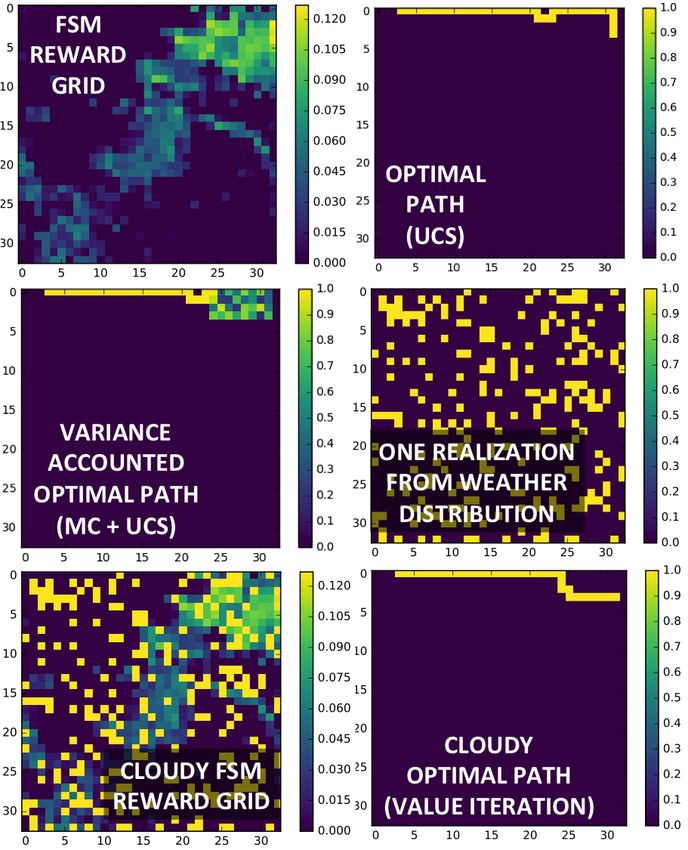
Table 2: CNN FSM Prediction Results.
                      Model                         Output Layer Feature Number     Tile or Full Image   Test Accuracy
                Nightlight Features                            4092                     Full Image            39%
        Image-Mean DeepSat Features + RR                         32                     Full Image          31.1 %
        Image-Mean DeepSat Features + RR                        256                     Full Image          30.8 %
               Direct CNN Learning                               32                         Tile            43.8 %
               Direct CNN Learning                              256                         Tile            45.0 %
               Direct CNN Learning                             1024                         Tile            46.5 %
     Direct Learning with Transfer Initialization               256                         Tile            46.4 %

der of less than 28 meters. In the future, it would be helpful      Sub-Problem 1: Finite Horizon Deterministic Ap-
to look at layer activations to determine the exact nature of    proach: Given our trained CNN H, we can use the constant
the features that are providing this predictive capacity. We     time prediction property of neural networks to traverse
also attempted transfer learning in a different manner, by       through each tile of the large image and create a 33 x 33
initializing the network with weights learned for DeepSat,       grid of predicted food security metrics in O(332 ) time. On
then continuing to train directly on the SustLab images and      this grid, we can start at a randomly chosen location and
associated stunting percentage. This procedure slightly out-     set up a Markovian search problem to find the tile with the
performed the pure Direct CNN Learning approach with a           lowest food metric (corresponding to the poorest region in
similar number of output layer features (256), but did not       our map) in the the least number of tile-to-tile moves (we
provide substantial improvement.                                 choose the number of moves as the metric of cost and define
                                                                 an optimal path as the least cost path, acknowledging that
                                                                 this path is not guaranteed to be unique). We use Uniform
Automated Satellite Tasking for Food Security                    Cost Search for this sub-problem.
              Measurements
Images to Reward Grids: Methodology and                             Sub-Problem 2: Finite Horizon Stochastic Approach:
                                                                 Aleatoric Uncertainty: In the previous model of the
Algorithms                                                       problem, we assumed that there are bounded and finite
The prediction pipeline obtained from the analysis above         horizons to our search space. We also spent time traversing
produces a food security metric (FSM) given an image,            each tile to calculate the food security metric to set up the
which becomes an input for an automated satellite task-          Markovian search problem. Inherent in the prediction task
ing algorithm. The FSM we use is the stunting percentage,        is an error incurred from the model having a finite accuracy.
which is normalized between 0 and 1 such that the numbers        As discussed above, a ridge regression is performed on the
closer to 0 denote food insecure regions whereas numbers         features produced by the CNN when the satellite image
closer to 1 denote regions with higher food security.            is the input. Therefore, the prediction of the FSM that is
    Figure 1 shows the project pipeline. In the prior sec-       obtained is the expected value of the FSM with variance
tions, we have discussed the first stage in this methodology     characterized by the coefficient of determination of the
where we train a model on the labeled images from DeepSat        regression fit. Recall that the coefficient of determination
(Saikat Basu 2015) and SustLab (Jean et al. 2016).               is the deviation from unity of the ratio of the residual sum
    This excercise helps us train a model that can predict       of squares and the total sum of squares. In a general form,
the FSMs over various sub-tiles of a larger image. To give       R2 can be seen to be related to the fraction of unexplained
an analogy, even though the Bay Area is food secure,             variance (FUV), since the ratio compares the unexplained
sub-regions within the Bay Area are not homogenous (i.e.         variance (variance of the model’s errors) with the total
Palo Alto versus East Palo Alto). In other words, transfer       variance (of the data). To get an estimate of this prediction
learning helps us go from a low resolution prediction to         variance, we use the following procedure:
a high resolution prediction. The process of extracting
a reward grid from the tiled image is the quantitative             Input: Images tagged with FSMs
description of this idea. The reward grid is produced by           for Image i = 1, 2, 3, . . . do
tiling the large image into small regions (making sure that            for On Image i, Tile t = 1, 2, 3, . . . do
the resolution of the training dataset for the model matches               Get FSM Prediction on tile t. Call it Pit
the resolution of the tiles) and then using the trained model          end for
to predict the FSM at each tile. Once this matrix has been             V ari = Variance of Pit over all t
created, we can look at the satellite tasking problem as a set     end for
of three sequentially linked sub-problems that each add a          Global Variance = σ 2 = Average of V ari over i
layer of complexity and uncertainty to solve the complete
problem. After pre-processing the SustLab images, we end         This variance characterizes up to the second moment of the
up with a 33 x 33 grid of 28 x 28 pixel images.                  background probabilistic distribution from which the reward
                                                                 grid is predicted. Sampling from this distribution and using
Figure 5: A schematic for the path from an image to generating an FSM
the Monte Carlo approach to calculate the relevant statistics
allows us to account for this uncertainty and calculate a
prediction error margin. This margin is calculated for the
predicted optimal path. The schematic in figure 5 and the
following procedure outlines our approach.
Input: Expected Reward Grid (µ), FSM Model Prediction
Variance (σ 2 )
Each tile on reward grid has added parameter onPath
Create a pathProbabilityMatrix of size equal to the size of
Figure 6: Visualization of the high resolution FSM predicted the reward grid. Initialize this matrix to zeros
by our model for Monte Carlo Realization r = 1, 2, 3, . . ., MCIters do
for On Reward Grid, Tile t = 1, 2, 3, . . . do
Reward Value at tile t sampled from N (µt , σ 2 )
Perform UCS on this realization of reward grid
Assign onPath = 1 to tiles that are on optimal path
Assign onPath = 0 to tiles that are not on path
end forpathProbabilityMatrix += onPathMatrix
end for
pathProbabilityMatrix /= MCIters
The path probability matrix assigns a probability of the
optimal path passing through a given tile. This probability
serves as a metric for a two-pronged validation of the
proposed model. One, a sharper path with less variance
implies that the trained model works well and is sufficient
for the given geographic area and builds confidence in our
prediction of FSMs. Two, a large variance indicates a mis-
match between the dataset on which training is conducted
versus the dataset on which prediction is attempted and
signals that either increasing the training database or adding
Figure 7: The Bayesian Network driven Markov Decision more geographically relevant data into the database would
Process. The Bayesian Network completely specifies the be advisable.
weather distribution which in turn completely specifies the
MDP Sub-Problem 3: Finite Horizon Stochastic Approach:
Epistemic Uncertainty: When satellite images are used, thenatural question that comes up is “What happens when the Conclusions and Future Work satellite view is occluded due to clouds?” To address this, In the end, we have accomplished several goals with this we propose a Markovian cloud cover model with Bernoulli work. First, we have shown that CNNs can accurately pre- probabilities for cloudy tiles. This model is completely spec- dict land cover classification on the DeepSat dataset with ified by the Bayesian network in Fig. 7. Thus, the future up to 87 % accuracy, which is on par with state-of-the-art step in the path search depends on the cloud cover (p(C)) results from other methods. Second, we have shown that that exists in the current state and the probability of tran- specification of a tile-scale CNN model either with direct sitioning (p(C t |C t−1 )) to a tile with/without cloud cover training on tiled SustLab images or via transfer initializa- given the current state of the cloud cover. An additional tion from a network trained on DeepSat data yields accu- binary variable is added to our minimal description of the racy of over 45 % on the test set, which outperforms the state to account for this. Note that both these probabilities baseline of 39 % generated by the current state-of-the-art. (which has a degree of freedom 3 for the 6 required probabil- The fact that this tile-scale CNN sourced from training on ities) can be estimated from historical data using a frequen- satellite-relevant datasets performs better than features ex- tist estimation strategy like maximum likelihood. A more tracted on the whole images from nightlight data implies physical weather model would incorporate spatial correla- that direct training on the metric of interest is indeed a use- tions and temporal statistics which can be modeled using ful contributor to improved accuracy. In the future, there are a deeper Bayesian network and a higher dimensional state- a variety of directions that the machine learning side of this space. Note that the runtimes of all the path search algo- work could be taken, including iterating over network archi- rithms used scale exponentially in the size of the state-space. tectures (GoogLeNet, ResNet, etc.) and obtaining additional For the purposes of this project and a proof-of-concept, data to allow for direct training on the larger-scale image. our limited validity model suffices. Once both p(C) and Use of either GoogLeNet or ResNet seems particularly al- p(C t |C t−1 ) are prescribed, the epistemic uncertainty is in- luring given their ability to incorporate (and simultaneously corporated into the problem specification and transforms the output) features at multiple different scales while incorpo- deterministic search problem into a Markov Decision Pro- rating skip connections, which may be particularly helpful cess. The state subgraph of the full MDP search graph is in ensuring that lower-level features are emphasized in the schematically shown in Fig. 7. On this MDP, value iter- classification layer. ation is performed so as to obtain the optimal movement On the satellite tasking portion of our project, we have policy given a state. It is instructive to note that once this shown that tasking under uncertainty can be handled both policy is computed, we do not need to re-compute the op- by UCS with a CNN-based probabilistic cost function and timal policy since prescribing the probability space of the MDPs driven by Bayesian networks. Future work on this MDP completely determines the optimal policy. This is the front should include incorporating physical, non-Markovian desired and required behavior for an algorithm that needs weather models to more accurately simulate actual satellite to be deployed on light hardwares - typical of satellites. conditions and identification of high-resolution satellite as- We perform this value iteration process on our MDP with sets that could benefit from these types of algorithms in prac- p(C = 1) = 0.2, p(C t = 1|C t−1 = 0) = 0.5 and tice. p(C t = 1|C t−1 = 1) = 0.5. The figure on the right in the middle row of Fig. 8 shows one particular realization of Acknowledgments the cloud cover. The figure on the left in the bottom of Fig. 8 shows the occluded view seen from a satellite due to the Prof. Stefano Ermon, Prof. Marshall Burke, and Stanford cloud cover in contrast to the clean view (top left of Fig. 8) Sustainability and Artificial Intelligence Lab that would otherwise be expected to be seen on a clear day. Value Iteration, in contrast to UCS tries to maximize the re- ward. The reward matrix described above is scaled affinely and linearly so that all values lie between 0 and 1 and the val- ues close to 1 signify lower food security. The goal is once again to reach the most food insecure point while traversing food insecure regions such the path is globally optimal in the sense that the locations traversed pass through the most food insecure regions within the horizon. In order to make sure that the path search avoids clouds, a zero value (high food security) is assigned to the locations where clouds ex- ist. Shown on the bottom right in Fig. 8 is the optimal path found when the realized cloud cover occludes the view. It is seen that the optimal policy learns to meander around the clouds. The optimal path in this case is also significantly dif- ferent than the optimal path obtained from UCS.
Figure 8: The results derived after an image has gone through the entire pipeline
References                                [Sandefur 2015] Sandefur, e. a. 2015. Benefits and costs of
[Alex Krizhevsky 2012] Alex Krizhevsky, Ilya Sutskever,            the data for development targets for the post-2015 develop-
 e. a. 2012. Imagenet classification with deep convolutional       ment agenda. J. Dev. Stud. 51, 116132.
 neural networks. Advances in neural information processing       [United Nations 2014] United Nations. 2014. A world that
 systems.                                                          counts: Mobilising the data revolution for sustainable devel-
[Chen and Nordhaus 2011] Chen, X., and Nordhaus, W. D.             opment.
 2011. Using luminosity data as a proxy for economic statis-      [World Bank 2015] World Bank.               2015.        Pov-
 tics. PNAS.                                                       calnet online poverty analysis tool, http:// ire-
[Devarajan 2013] Devarajan. 2013. Rev. Income Wealth 59,           search.worldbank.org/povcalnet/.
 S9S15.
[Dunnmon et al. 2019] Dunnmon, J.; Ganguli, S.; Hau, D.;
 and Husic, B. 2019. Predicting us state-level agricultural
 sentiment as a measure of food security with tweets from
 farming communities. arXiv preprint arXiv:1902.07087.
[Ganguli, Garzon, and Glaser 2019] Ganguli, S.; Garzon, P.;
 and Glaser, N. 2019. Geogan: A conditional gan with recon-
 struction and style loss to generate standard layer of maps
 from satellite images. arXiv preprint arXiv:1902.05611.
[Henderson, Storeygard, and Weil 2011] Henderson,          V.;
 Storeygard, A.; and Weil, D. N. 2011. A bright idea for
 measuring economic growth. Am. Econ. Rev. 101:194–199.
[Jean et al. 2016] Jean, N.; Burke, M.; Xie, M.; Davis,
 W. M.; Lobell, D. B.; and Ermon, S. 2016. Combining
 satellite imagery and machine learning to predict poverty.
 Science Magazine 353(6301):790–794.
[Jerven 2013] Jerven. 2013. Poor numbers: How we are mis-
 led by african development statistics and what to do about it.
 Cornell Univ. Press.
[Jerven 2014] Jerven. 2014. Benefits and costs of the data for
 development targets for the post-2015 development agenda.
 Data for Development Assessment Paper Working Paper,
 September (Copenhagen Consensus Center, Copenhagen,
 2014).
[Karen Simonyan 2014] Karen Simonyan, e. a. 2014. Very
 deep convolutional networks for large-scale image recogni-
 tion. arXiv.
[Meyer 2014] Meyer, e. a. 2014. Silicon Valley’s new spy
 satellites. The Atlantic.
[Perez et al. 2019] Perez, A.; Ganguli, S.; Ermon, S.; Azzari,
 G.; Burke, M.; and Lobell, D. 2019. Semi-supervised multi-
 task learning on multispectral satellite images using wasser-
 stein generative adversarial networks (gans) for predicting
 poverty. arXiv preprint arXiv:1902.11110.
[Pinkovskiy 2017] Pinkovskiy, M. L. 2017. Growth discon-
 tinuities at borders. J. Econ. Growth.
[Romero, Gatta, and Camps-Valls 2014] Romero, A.; Gatta,
 C.; and Camps-Valls, G. 2014. Unsupervised deep feature
 extraction of hyperspectral images. In IEEE GRSS Work-
 shop on Hyperspectral Image and Signal Processing (WHIS-
 PERS). IEEE, volume 6.
[Safyan 2015] Safyan, e. a. 2015. Overview of the planet
 labs constellation of earth imaging satellites. ITU Sympo-
 sium/Workshop, Prague.
[Saikat Basu 2015] Saikat Basu, Sangram Ganguly, e. a.
 2015. Deepsat a learning framework for satellite imagery.
 arXiv.
You can also read