Adaptive Illumination based Depth Sensing using Deep Learning

Adaptive Illumination based Depth Sensing using Deep Learning

 Qiqin Dai1 , Fengqiang Li2 , Oliver Cossairt2 , and Aggelos K Katsaggelos2
 1
 Geomagical Labs
 2
 Northwestern University
arXiv:2103.12297v1 [cs.CV] 23 Mar 2021

 Abstract tance, and occlusion problems can also be minimized with
 them. Compared to indirect ToF cameras, LiDAR has a
 Dense depth map capture is challenging in existing ac- much longer imaging range (eg., tens of meters) with a high
 tive sparse illumination based depth acquisition techniques, depth precision (eg., mm) which enables it to be a competi-
 such as LiDAR. Various techniques have been proposed to tive depth sensor. LiDAR has been widely used for machine
 estimate a dense depth map based on fusion of the sparse vision applications, such as, navigation in self-driving cars
 depth map measurement with the RGB image. Recent ad- and mobile devices (e.g., LiDAR sensor on Apple iPhone
 vances in hardware enable adaptive depth measurements 12).
 resulting in further improvement of the dense depth map Most LiDAR sensors measure one point of the object at
 estimation. In this paper, we study the topic of estimat- a time, and rely on raster scanning to generate a full 3D im-
 ing dense depth from depth sampling. The adaptive sparse age of the object, which limits its acquisition speed. In order
 depth sampling network is jointly trained with a fusion net- to produce a full 3D image of an object with a reasonable
 work of an RGB image and sparse depth, to generate op- frame rate of a mechanical scanning scheme, LiDAR can
 timal adaptive sampling masks. We show that such adap- only provide a sparse scanning with two adjacent measur-
 tive sampling masks can generalize well to many RGB and ing points being far away. This leads to very limited spatial
 sparse depth fusion algorithms under a variety of sampling resolution with LiDAR sensor. To increase LiDAR’s spa-
 rates (as low as 0.0625%). The proposed adaptive sampling tial resolution and acquire more structural information of
 method is fully differentiable and flexible to be trained end- the scene, other high-spatial-resolution imaging modalities,
 to-end with upstream perception algorithms. such as RGB, are used to be fused with LiDAR’s depth im-
 ages [56, 37]. Traditionally, LiDAR sensors perform raster
 scanning following a regular grid to produce a spatially uni-
 1. Introduction formly spaced depth map. Recently, researchers explore the
 LiDAR scanning or sampling patterns and co-optimize the
 Depth sensing and estimation is important for many ap- sensor’s sampling pattern with a fusion pipeline to further
 plications, such as autonomous driving [35], augmented re- increase its performance [4]. Pittaluga et al. [45] implement
 ality (AR) [20], and indoor perception [18]. on a real hardware device adaptive scanning patterns for the
 Based on the principle of operation, we can roughly LiDAR sensor by using a MEMS mirror. They co-optimize
 divide current depth sensors into two categories: (1) the scanning hardware and the fusion pipeline with an RGB
 Triangulation-based depth sensors (eg., stereo [26]) and (2) sensor to increase LiDAR’s performance.
 Time-of-flight (ToF) based depth sensors (including direct In this paper, we study the topic of adaptive depth sam-
 ToF LiDAR sensor and indirect ToF cameras [14]). The pling and depth map reconstruction. First, we formulate
 depth precision of triangulation-based depth sensors varies the pipeline of joint adaptive depth sampling and depth
 directly with the baseline and inversely with standoff dis- map estimation. Then, we propose a deep learning (DL)
 tance. Therefore, large baselines are required to realize based algorithm for adaptive depth sampling. We show that
 higher depth precision at longer standoff distances. More- the proposed adaptive depth sampling algorithm can gen-
 over, the geometric arrangement of the sensor components eralize well to many depth estimation algorithms. Finally,
 can lead to occlusion problems, which are not plausible we demonstrate a state-of-the-art depth estimation accuracy
 in depth sensing. On the contrary, the depth precision of compared to other existing algorithms.
 ToF-based depth sensors is independent of the standoff dis- Our contribution is summarized as follows:

 4321

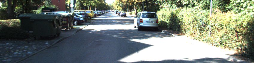
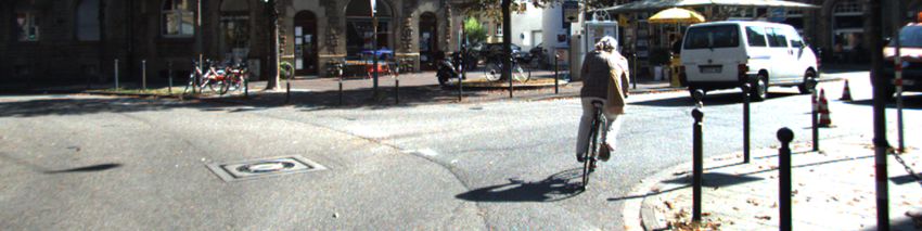
2.1. Depth Estimation
 Given RGB images, early depth prediction methods re-
 lied on hand-crafted features and probabilistic graphics
 RGB Image models. Karsch et al. [27, 28] estimate the depth based
 on querying an RGBD image database. A Markov random
 field model is applied in [51] to regress depth from a set of
 image features. Recently deep learning (DL) and convolu-
 tional neural networks (CNNs) have been applied to learn
 Predicted Depth using Randomly Sampled Depth, RMSE: 2052.5
 the mapping from single RGB images to dense depth maps
 [12, 11, 32, 15, 46, 2, 33, 57]. These DL based approaches
 achieve state-of-the-art performance because better features
 are extracted and better mappings are learned from large-
 Predicted Depth using Adaptively Sampled Depth, RMSE: 1146.9 scale datasets [53, 16, 49].
 Given sparse depth measurements, traditional image fil-
 tering and interpolation techniques [30] can be applied to
 reconstruct the dense depth map. Hawe [19] and Liu [39]
 study the sparse depth map completion problem from the
 Depth Ground Truth compressive sensing aspect. DL techniques have also been
 applied to the sparse depth completion problem. A sparse
Figure 1. LiDAR systems is able to capture accurate sparse depth depth map can either be fed into conventional CNNs [43]
map (bottom). Reducing the number of samples we are able to in-
 or sparsity invariant CNNs [55]. When the sampling rate is
crease the capture framerate. RGB image (top) can be fused with
 low, the sparse depth map completion task is challenging.
the captured sparse depth data and estimate a dense depth map.
We demonstrate that choosing the sampling location is important If both RGB images and sparse depth measurements are
to the accuracy of the estimated depth map. Under 0.25% sam- provided, traditional guided filter approaches [34, 3] can be
pling rate (with respect to the RGB image), using the same depth applied to refine the depth map. Optimization algorithms
estimation method [56], the depth map estimated from the adap- that promote depth map priors while maintaining fidelity to
tively sampled sparse depth (third row) is more accurate than the the observation are proposed in [40, 10, 41]. Various DL
depth map estimated from random samples (second row). based methods have been developed [43, 42, 56, 6, 25, 59,
 61, 52]. During training and testing, most DL approaches
 are trained and tested using random or regular grid sam-
 • We propose an adaptive depth sensing framework pling masks. Because depth completion is an active re-
 which benefits from active sparse illumination depth search area, we do not want to limit our adaptive sampling
 sensors, such as LiDAR and sparse dot-pattern struc- method to a specific depth estimation method.
 tured light sensors.
 2.2. Sampling Mask Optimization
 • We propose a superpixel segmentation based adaptive
 sampling mask prediction network and experimentally Irregular sampling [7, 44, 5] is well studied in the com-
 show better sampling performance compared to exist- puter graphics and image processing literature to achieve
 ing sampling methods. good representation of images. Making the sampling dis-
 tribution adaptive to the signal further improves representa-
 • We propose a differentiable sampling layer, that trans- tion performance. Eldar et al. [13] proposed a farthest point
 lates the estimated sampling locations (x, y coordi- strategy which performs adaptive and progressive sampling
 nates) into a binary sampling mask. of an image. Inspired by the lifting scheme of wavelet
 generation, several progressive image sampling techniques
 • We demonstrate that the proposed adaptive sampling were proposed [9, 47]. Ramponi et al. [48] applied a mea-
 method can generalize well to many depth estimation sure of the local sample skewness. Lin et al. [36] utilized
 algorithms without fine tuning, thus establishing the the generalized Ricci curvature to sample grey scale images
 effectiveness of the proposed sampling method. as manifolds with density. A kernel construction technique
 is proposed in [38]. Taimori et al. [54] investigated space-
2. Related Work frequency-gradient information of image patches for adap-
 tive sampling.
 In this section, we review work on algorithm-based depth Specific reconstruction algorithms are needed for each
estimation and sampling mask optimization and clarify the of these irregular or adaptive sampling methods [7, 13, 47,
relationship to our proposed method. 9, 48, 36, 38, 54] to reconstruct the fully sampled signal.

 4322

NetM

 RGB Image Sampling Mask * NetE

 Sampled Sparse Depth Predicted Depth

 Depth Ground Truth

Figure 2. The proposed pipeline contains two submodules, adaptive depth sampling (N etM ) and depth reconstruction (N etE). The binary
adaptive sampling mask is generated by N etM based on the RGB image. Then, the LiDAR system samples the scene based on this binary
sampling mask and generates the sampled sparse depth map. Finally, both the RGB image and the sampled sparse depth map are input to
N etE to estimate a dense depth map.

Furthermore, handcrafted features are applied to these sam- sampling networks [23, 58] and depth estimation networks
pling methods. Finally, these sampling techniques are all [7, 13, 47, 9, 48, 36, 38, 54] could adapt the sampling net-
applied to the same modality (RGB or grey scale image). work to depth estimation and obtain improved reconstruc-
Recently, Dai et al. [8] applied DL technique to the adap- tion accuracy. Bergman et al. [4] warp an uniform sampling
tive sampling problem. The adaptive sampling network is grid to generate the adaptive sampling mask. The warping
jointly optimized with the image inpainting network. The vectors are computed utilizing DL based optical flow esti-
sampling probability is optimized during training, and bi- mated from the RGB image. A spatial distribution prior is
narized during testing. Good performance is demonstrated enforced by the initial uniform sampling grid. End-to-end
for X-ray fluorescence (XRF) imaging at a sampling rate as optimization of the sampling and depth estimation networks
low as 5%. Kuznetsov et al. [31] predicted adaptive sam- is performed and good depth reconstruction is obtained un-
pling maps jointly with reconstruction of Monte Carlo (MC) der low sampling rates. In the pipeline of [4], there are 4
rendered images using DL. A differentiable render simula- sub-networks, 2 for sampling and the other 2 for depth es-
tor with respect to the sampling map was proposed. Huijben timation. They are jointly trained but only the final depth
et al. [21, 22] proposed a task adaptive compressive sens- estimation results are demonstrated. The whole pipeline is
ing pipeline. The sampling mask is trained with respect to bulky and expensive. More importantly, it is hard to ac-
a specific task and is fixed during imaging. Gumbel-max cess if the improvement on depth estimation comes from the
trick [17, 24] is applied to make the sampling layer differ- sampling part or the depth estimation part of the pipeline. In
entiable. this paper, we decouple these two parts and study each in-
 dividual module to better understand their contribution to-
 All of the above DL based sampling methods predict a wards the final depth estimate. Finally, a bilinear sampling
per pixel sampling probability [8, 21, 22] or a sampling kernel is applied in [4] to make the optimization of the sam-
number [31]. Good sampling performance has not been pling locations differentiable. On the contrary, we propose
demonstrated under extreme low sampling rates (< 1%). a novel differentiable relaxation of the sampling procedure
Directly enforcing priors on sampling locations is effec- and show its advantages over the bilinear sampling kernel.
tive when the sampling rate is low. This requires the adap-
tive sampling network to predict sampling locations ((x, y)
coordinates) directly and the sampling process be differ- 3. Method
entiable. For the RGB and sparse depth adaptive sam- 3.1. Problem Formulation
pling task, Wolff et al. [58] use the SLIC superpixel tech-
nique [1] to segment the RGB image and sample the depth As shown in Figure 2, the input RGB image is denoted
map at the center of mass of each superpixel. A bilateral by I. The mask generation network N etM produces a bi-
filtering based reconstruction algorithm is proposed to re- nary sampling mask B = N etM (I, c), where c ∈ [0, 1]
construct the depth map. A spatial distribution prior is is the predefined sampling rate. Elements in B equal to
implicitly enforced by superpixel segmentation, resulting 1 correspond to sampling locations and 0 to non-sampling
in good sampling performance under low sampling rates. location. Then the LiDAR system is sampling depth ac-
The sampling and reconstruction methods are not opti- cording to B and produces the measured sparse depth map
mized jointly, leaving room for improvement. In this paper, D0 . In synthetic experiments, if the ground truth depth map
we show that jointly training recent DL based superpixel D is given, the measured sparse depth map D0 is obtained

 4323

1x1 conv upsample upsample upsample upsample bilinear
 ResNet18 3x3 conv upsample
 batch-norm layer layer layer layer
 4@ 1@
 32@ 16@ 1@
 240x960 512@ 256@ 128@ 240x960
 64@ 128x480 128x480
 8x30 8x30 16x60 64x240
 32x120

 Encoder Decoder

Figure 3. Network architecture for the depth estimation network (N etE). The network consists of an encoder and a decoder. The RGB
image and the corresponding sparse depth image are concatenated at the input.

according to ure 2, N etM adapts to the task of depth sampling after be-
 ing jointly trained with N etE.
 D0 = D B=D N etM (I, c), (1) Superpixel with fully convolutional networks (FCN) [60]
 is one of the DL based superpixel techniques. It predicts
where is the element-wise product operation. The recon- the pixel association map Q given an RGB image I. Its
structed depth map D̄ is obtained by the depth estimation encoder-decoder network architecture is shown in Figure 4.
network N etE, that is, Similarly to the SLIC superpixel method [1], a combined
 loss that enforces similarity property of pixels inside one
 superpixel and spatial compactness is applied. Readers can
 D̄ = N etE(I, D0 ) = N etE(I, D N etM (I, c)). (2)
 refer to [60] for more details.
 The overall adaptive depth sensing and depth estimation Given an RGB image I with spatial dimensions (H, W ),
pipeline is shown in Figure 2. End-to-end training can be under the desired depth sampling rate c, we have Np =
applied on N etM and N etE jointly. The adaptive depth H · W pixels and Ns = c · H · W superpixels. The
sampling strategy is learned by N etM , while N etE esti- sampled depth location is the weighted mass center of
mates the final dense depth map. An informative sampling each superpixel. We denote the subset of pixels as P =
mask is beneficial to depth estimation algorithms in gen- {P0 , ..., PNs −1 }, where Pi is a set of pixels associated with
eral, not just to N etE. During testing, we can replace the superpixel i. Pixel p’s CIELAB color property and (x, y)
inpainting network N etE with other depth estimation algo- coordinates are denoted by f (p) ∈ R3 and c(p) ∈ R2 , re-
rithms. Network architectures and training details of N etE spectively. The loss function is given by
and N etM are discussed in the following subsections.
 X
3.2. Depth Estimation Network N etE LSLIC (f , Q) = kf (p) − f 0 (p)k2 + mkc(p) − c0 (p)k2 .
 p∈P
 We use the network architecture in [43] for the depth es- (3)
timation network, as shown in Figure 3. The network is Here we have
an encoder-decoder pipeline. The encoder takes a concate- P P
 f (p)qs (p) c(p)qs (p)
nated I and D0 as input (4 channels) and encodes them into us =
 p∈Ps
 P , ls =
 p∈Ps
 P , (4a)
latent features. The decoder takes the low spatial resolution p∈Ps qs (p) p∈Ps qs (p)
feature representation and outputs the restored depth map
 X X
 f 0 (p) = us qs (p), c0 (p) = ls qs (p), (4b)
D̄ = N etE(I, D0 ). s∈Np s∈Np
 Because method [43] is differentiable with respect to D0
(unlike [6]) and its network architecture is standard with- where m is a weight balancing term between the CIELAB
out customized fusion modules [25, 56, 6], we choose it as
N etE and jointly train N etM with it according to Figure 2.
We found out that the trained N etM can generalize well to
other depth estimation methods during testing.

3.3. Sampling Mask Generation Network N etM
 Existing irregular sampling techniques [13, 5] and adap-
tive depth sampling methods [4, 58] explicitly or implic-
itly make sampling points evenly distributed spatially. Such
 Input RGB Output association
prior is important when the sampling rate is low. In- Image Map 

spired by the SLIC superpixel [1] based adaptive sampling
method [58], we propose to utilize recent DL based super- Figure 4. Superpixel FCN [60]’s encoder-decoder network archi-
pixel networks [60, 23] as N etM . As demonstrated in Fig- tecture.

 4324

2 2
 e−ρi /t
 …

 …

 …
 ki = P 2 2
 . (6)
 l! l" w# l! e−ρj /t
 … … … … … … .
 j∈NW
 " !

 w" w! w"
 When the temperature parameter t → 0, the sampled
 …

 …

 …
 depth value ds is equal to the depth value dn of the nearest
 pixel wn . When t is large, the soft sampled depth value ds is
 (a) (b) (c) different from dn . We gradually reduce t during the training
 process. During testing, we find the nearest neighbor pixel
Figure 5. Illustration of the sampling approximation. (a) We find a wn of ls and sample the depth value dn at wn .
local window W of ls and compute distance ρi . (b) We represent
ls ’s depth value ds as a linear combination of local window W ’s 3.5. Training Procedures
depth values. (c) During testing, we sample the depth value at the
nearest neighbour wn of ls .
 Given the training dataset consisting of the aligned RGB
 image I and the ground truth depth map D, we first train
 N etE by minimizing the depth loss,
color similarity and spatial compactness, Np is the set of su-
 Ldepth = kD − N etE(I, D0 )k2 , (7)
perpixels surrounding p, qs (p) is the probability of a pixel
p being associated with superpixel s and is derived from where D0 is obtained by applying a random sampling mask
the associate map Q, us ∈ R3 and ls ∈ R2 are the color on D with sampling rate c.
property and locations of superpixel s, f 0 (p) ∈ R3 and Then we initialize the superpixel network N etM using
c0 (p) ∈ R2 are respectively the reconstructed color prop- the RGB image I. LSLIC is minimized according to Equa-
erty and location of pixel p. tion 3. The initialized N etM approximates the SLIC super-
 pixel segmentation on RGB image. If we sample the depth
3.4. Soft Sampling Approximation
 value on ls of each superpixel, the sampling pattern would
 Defined in Equation 4(a), we denote the collection of be similar to [58].
ls (), s = 0, ..., Ns − 1 , as S. Depth values at loca- Finally, we jointly train N etE and N etM in Figure 2 by
tions S would be measured during the depth sampling. In minimizing
order to train N etM and N etE jointly, the sampling op- L = Ldepth + q · LSLIC , (8)
eration g, which computes the sampled sparse depth map where q is the weighting terms of LSLIC . The SSA trick
D0 from depth ground truth D and sampling location S, shown in Figure 5 is applied and the temperature parameter
D0 = g(D, S), needs to be differentiable with respect to t gradually decreases during training.
S. Unfortunately, such sampling operation g is not differen- We fix N etE when training N etM . Optimizing N etE
tiable in nature. Bergman et al. [4] apply a bilinear sampling and N etM simultaneously would obtain optimal depth re-
kernel to differentiably correlate S and D0 . The computed construction accuracy [4]. However, similarly to [8], we
gradients rely on the 2 × 2 local structure of the ground would utilize other depth estimation methods than N etE
truth depth map D. The computed gradients are not stable during testing. We want to make the adaptive depth sam-
when the sampling location is sparse. Thus limited sam- pling mask be general and applicable to many depth esti-
pling performance is obtained. We propose a soft sampling mation algorithms.
approximation (SSA) strategy during training. SSA utilizes
a larger window size compared to the bilinear kernel and 4. Experimental Results
achieves better sampling performance.
 As shown in Figure 5, during training, given a sampling 4.1. Implementation Details
location ls ∈ S, we find a local h×w window W around ls . We use the KITTI depth completion dataset [55] for our
The depth value ds at ls is a weighted average of the depth experiments. It consists of aligned ground truth depth maps
values in W , (from LiDAR sensor) and RGB images. The original KITTI
 X training and validation set split is applied. There are 42949
 ds = ki di , (5) and 3426 frames in the training and validation sets, respec-
 i∈NW
 tively. We only use the bottom center crop 240 × 960 of the
where NW includes the indices of all pixels in W , wi is the images because the LiDAR sensor has no measurements at
ith pixel’s location in W , di is the depth value of wi , the the upper part of the images.
weights ki are computed according to the Euclidean dis- The ground truth depth maps are not dense because they
tance ρi between ls and wi , scaled by a temperature param- are measured by a velodyne LiDAR device. In order to per-
eter t, form adaptive depth sampling, we need dense depth maps to

 4325

MAE (mm)
 c=1% c=0.25% c=0.0625%
 FusionNet SSNet N etE Colorization FusionNet SSNet N etE Colorization FusionNet SSNet N etE Colorization
 Random 324.8 466.6 425.7 764.6 488.6 654.9 557.1 1390.7 798.5 1021.1 779.4 2517.5
 Poisson 324.1 451.8 409.6 711.5 455.8 621.2 537.5 1314.1 736.2 901.0 743.1 2428.4
 SPS 297.2 439.9 388.1 654.3 436.9 594.2 507.8 1197.2 713.8 865.2 724.5 2175.9
 DAL 295.8 447.4 390.1 683.4 432.5 599.1 504.8 1239.7 694.4 838.4 710.2 2230.7
 N etM 285.0 423.1 380.1 656.2 404.3 562.2 477.5 1189.2 634.9 778.0 652.2 2265.8
 RMSE (mm)
 c=1% c=0.25% c=0.0625%
 FusionNet SSNet N etE Colorization FusionNet SSNet N etE Colorization FusionNet SSNet N etE Colorization
 Random 1060.0 1221.6 1294.8 1984.4 1476.0 1709.9 1704.3 3087.3 2135.6 2505.6 2262.61 4749.8
 Poisson 1010.1 1140.2 1193.3 1844.8 1375.6 1589.1 1596.8 2897.3 2013.1 2256.0 2151.4 4508.6
 SPS 1039.1 1124.3 1160.5 1742.9 1360.1 1559.7 1553.1 2718.1 1993.8 2215.0 2141.5 4161.1
 DAL 969.9 1115.1 1177.5 1784.3 1336.1 1548.1 1532.1 2772.6 1937.6 2128.3 2085.7 4242.3
 N etM 939.4 1074.9 1131.3 1725.9 1239.7 1436.8 1422.4 2584.5 1732.4 1930.5 1896.7 3972.9
Table 1. Depth sampling and estimation results on KITTI test dataset. Random, Poisson [5], SPS [58], DAL [4] and proposed N etM
sampling strategies are compared utilizing N etE [43], FusionNet [56], SSNet [42], and Colorization [34] depth estimation algorithms.
MAE and RMSE metrics are reported. Best results are shown in bold. The results shown are averaged over a set of 3426 test frames.

sample from. Similarly to [4], a traditional image inpainting methods. Learning rate of N etM is assigned to be equal to
algorithm [34] is applied to densify the depth ground truth. 10−4 and is reduced by 50% every 10 epochs. SGD opti-
During evaluation, we compare the estimated dense depth mizer with momentum 0.9 is used. We found that 50 epochs
maps to the original sparse ground truth depth maps. in total are adequate for converge.
 During the training of N etE, we follow Ma et al.’s Our proposed adaptive depth sampling framework
setup [43]. The batch size is set equal to 16. The ResNet is implemented in PyTorch and our implementation
encoder in Figure 3 is initialized with pretrained weights is available at: https://github.com/usstdqq/
using the ImageNet dataset [50]. Stochastic gradient de- adaptive-depth-sensing.
scent (SGD) optimizer with momentum 0.9 is used. We
train 100 epochs in total. The learning rate is set to be 4.2. Performance on Adaptive Depth Sensing and
equal to 0.01 at first and reduced by 80% at every 25 Estimation
epochs. N etE is trained individually under different sam- For the adaptive depth sampling and estimation task,
pling rates c = 1%, 0.25% and 0.0625% using random we demonstrate the advantages of our proposed adaptive
sampling masks. We also train FusionNet [56] and SS- sampling mask N etM , over the use of random and Pois-
Net [42] under different sampling rates using random sam- son [5] sampling masks, as well as other state-of-the-art
pling masks. The same training procedure in their original adaptive depth sampling methods, such as SuperPixel Sam-
papers are used. They serve as alternative depth estimation pler (SPS) [58] and Deep Adaptive Lidar (DAL) [4].
methods. Random, Poisson, SPS [58], DAL [4] and proposed
 We test the proposed sampling algorithm under 3 sam- N etM sampling methods are applied to the 3426 test
pling rates, c = 1%, 0.25% and 0.0625%. They correspond frames from the KITTI validation set. Sampling rates
to Ns = 2304, 576 and 144 depth samples (superpixels) in c = 1%, 0.25% and 0.0625% are tested. For the depth
the 240 × 940 image. N etM is configured to output the estimation methods, DL based methods N etE [43], Fu-
desired number of samples. During the training of N etM , sionNet [56], SSNet [42] and traditional method Coloriza-
we pretrain it using the SLIC loss. m in Equation 3 is set tion [34] are used to estimate the fully sampled depth map
equal to be 1. ADAM optimizer [29] is applied. Learning from the sampled depth map and RGB image. It’s noted
rate is set to be 5 × 10−5 . We train 100 epochs in total. that all the DL based depth estimation methods are trained
 After N etM is initialized, we finally jointly train N etM using random sampling masks and the same KITTI training
and N etE according to Figure 2. Loss defined in Equa- dataset.
tion 8 is optimized with q equal to 10−6 , resulting in Ldepth The average Root Mean Square Error (RMSE) and Mean
being equal to about 10 times of q · LSLIC in value. The Absolute Error (MAE) over all 3426 test frames are shown
window size of the soft depth sampling module is equal to in Table 1. First, under all three sampling rates, the
5. Temperature t defined in Equation 6 decreases from 1.0 proposed N etM mask outperforms the random, Poisson,
to 0.1 linearly during training. Batch size is set equal to 8 SPS and DAL masks consistently over all depth estimation
and this is the largest batch size we can use for both N etM methods in terms of RMSE and MAE. This demonstrates
and N etE in an NVIDIA 2080Ti GPU (11GB memory). As the effectiveness of our proposed adaptive depth sampling
discussed in Section 3.5, N etE is fixed during the training network. Furthermore, N etM is jointly trained with N etE
to make N etM generalize well to other depth estimation and it still performs well with other depth estimation meth-

 4326

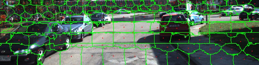
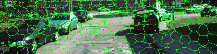
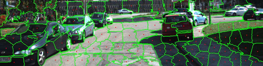
RGB Image Depth Ground Truth

RMSE: 1612.2 RMSE: 1913.8 RMSE: 1852.0 RMSE: 3604.3
Random Sampling + FusionNet Reconstruction Random Sampling + SSNet Reconstruction Random Sampling + N etE Reconstruction Random Sampling + Colorization Reconstruction

RMSE: 1617.8 RMSE: 1873.0 RMSE: 1965.0 RMSE: 3260.5
Poisson Sampling + FusionNet Reconstruction Poisson Sampling + SSNet Reconstruction Poisson Sampling + N etE Reconstruction Poisson Sampling + Colorization Reconstruction

RMSE: 1559.9 RMSE: 1902.9 RMSE: 1848.4 RMSE: 3280.7
SPS Sampling + FusionNet Reconstruction SPS Sampling + SSNet Reconstruction SPS Sampling + N etE Reconstruction SPS Sampling + Colorization Reconstruction

RMSE: 1561.6 RMSE: 1883.8 RMSE: 1839.4 RMSE: 3376.6
DAL Sampling + FusionNet Reconstruction DAL Sampling + SSNet Reconstruction DAL Sampling + N etE Reconstruction DAL Sampling + Colorization Reconstruction

RMSE: 1248.5 RMSE: 1531.2 RMSE: 1505.1 RMSE: 3028.1
N etM Sampling + FusionNet Reconstruction N etM Sampling + SSNet Reconstruction N etM Sampling + N etE Reconstruction N etM Sampling + Colorization Reconstruction

Figure 6. Visual comparison of the estimated depth maps. Random, Poisson, SPS, DAL, and N etM sampling masks at sampling rate
c = 0.25% are applied and shown in the 2nd − 6th rows, respectively. The first row includes the RGB image and the ground truth depth
map. Sampling locations are indicated using black dots. FusionNet, SSNet, N etE and Colorization depth estimation methods are used to
perform depth estimation and generate the depth maps of 1st − 4th columns, respectively. RMSE is computed for each depth map with
respect to the ground truth depth map.

ods, demonstrating that it can generalize well to other depth FusionNet SSNet N etE
 c Kernel MAE RMSE MAE RMSE MAE RMSE
estimation methods. The performance advantage of N etM Bilinear 290.5 948.4 436.3 1086.7 383.0 1138.8
 1%
is not tied to any specific depth estimation method. Fi- SSA 285.0 939.4 423.1 1074.9 380.1 1131.3
nally, it can be concluded that the smaller the sampling rate, Bilinear 431.1 1285.3 590.1 1487.5 494.1 1466.0
 0.25%
 SSA 404.3 1239.7 562.2 1436.8 477.5 1422.4
the larger the advantage of N etM compared to other sam- 0.0625%
 Bilinear 809.1 2161.4 989.2 2457.4 781.6 2253.0
pling algorithms. This implies that N etM is able to handle SSA 634.9 1732.4 778.0 1930.5 652.2 1896.7

challenging depth sampling tasks (extremely low sampling
 Table 2. Using SSA and Bilinear kernel during training results dif-
rates).
 ferent sampling quality of N etM .
 The visual quality comparison of various sampling
strategies and depth estimation methods is shown in Fig-
ure 6. For sampling rate equal to c = 0.25%, we can ure 7, we visualize the superpixel segmentation results and
observe the advantages of the proposed N etM mask over the derived sampling locations for SLIC, FCN and N etM
all other sampling masks by comparing the resulting depth when c = 0.0625%. SLIC and FCN segment the input
maps by the same depth estimation algorithm. N etM sam- RGB image based on the color similarity and preserve spa-
ples densely around the end of the road, trees and billboard, tial compactness. The segmentation density is spatially ho-
resulting in accurate depth estimation in such areas. Com- mogeneous. N etM is jointly trained with N etE, thus it
pared to other adaptive sampling algorithms, such as SPS has knowledge of distance given the RGB input image. Dis-
and DAL, N etM samples more densely on distance ob- tance objects in the image are sampled denser. It also seg-
jects, making the estimated depth more accurate. SPS uses ments sparsely the pavement and grass areas. Such near
SLIC [1] to segment the RGB image and such segmentation objects as cars are segmented denser compared to the pave-
can not obtain distance information from the RGB images. ment and grass areas. We also observe that N etM segmen-
DAL estimates a smooth motion field to warp a regular sam- tation does not preserve color pixel boundaries as well as
pling grid. When the scene is complicated, it is not flexible FCN, which is expected as N etM also minimizes the depth
enough to warp a regular sampling grid to optimal location. estimation loss besides the SLIC loss in Equation 8.
 N etM is initialized with RGB images trained FCN [60]
superpixel network using the SLIC loss (Equation 3). 4.3. Effectiveness of Soft Sampling Approximation
SPS [58] uses the SLIC superpixel technique to segment
the RGB images. Sampling locations are determined by the In Section 3.4, we propose the use of SSA to make the
weighted mass center of superpixels. Different superpixel sampling process differentialble during training. Such dif-
segmentations result in different sampling quality. In Fig- ferentiable sampling approximation is necessary to jointly

 4327

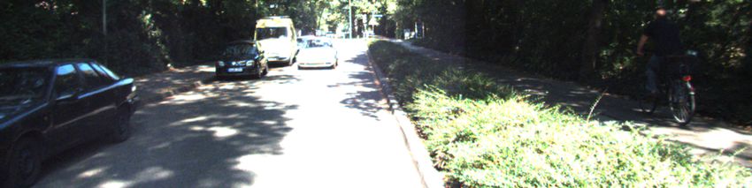
RGB Image RGB Image
 SLIC

 RMSE: 1039.0 RMSE: 1170.8
 SPS Sampling + SPS Reconstruction SPS Sampling + SPS Reconstruction

 RMSE: 1350.0 RMSE: 1239.1
 DAL Sampling + DAL Reconstruction DAL Sampling + DAL Reconstruction
 FCN

 RMSE: 871.9 RMSE: 1022.5
 N etM Sampling + FusionNet Reconstruction N etM Sampling + FusionNet Reconstruction
 N etM

 RMSE: 847.2 RMSE: 912.8
 N etM ∗ Sampling + FusionNet* Reconstruction N etM ∗ Sampling + FusionNet* Reconstruction

Figure 7. Visual comparison of different superpixel segmentation Depth Ground Truth Depth Ground Truth
and sampling location. Segmentation boundaries are plotted in
green and sampling locations are plotted in red. Figure 8. Visual comparison of different depth sampling and esti-
 mation methods.

train N etM with N etE. Compared to the 2×2 bilinear ker-
nel based differentable sampling in [4], the proposed SSA with N etE and FusionNet is trained using random masks.
provides better sampling performance. In order to show the Similarly to DAL, N etM and FusionNet can also be op-
advantages of SSA, we replace the SSA sampling of N etM timized simultaneously. Starting from the N etE trained
by the bilinar kernel based sampling and perform the exact N etM and random mask trained FusionNet, we alterna-
same training procedures. As demonstrated in Table 2, the tively train N etM and FusionNet and denote the trained
lower the sampling rate, the bigger the advantage of SSA networks by N etM ∗ and FusionNet*, respectively. The
over the bilinear kernel sampling. When sampling points joint depth sampling and reconstruction results are shown
are sparse, the gradients derived from a 2 × 2 local window in Table 3. We also compare with the sampling and re-
are too small to train N etM effectively. We empirically construction methods proposed in SPS and DAL. N etM ∗
found that the 5 × 5 window size for SSA provides reason- with FusionNet* slightly outperforms N etM with Fusion-
able sampling performance under all sampling rates. Net and achieves the best accuracy. Utilizing random sam-
 pling masks during the training of depth estimation meth-
4.4. End To End Depth Estimation Performance ods (FusionNet, SSNet, N etE) makes the methods robust
 to other sampling patterns in testing. We also found that
 In Table 1, FusionNet [56] achieves the best depth esti- N etM trained using different depth estimation methods has
mation performance under various of sampling masks. The similar sampling patterns. So simultaneously training the
proposed global and location information fusion is effective sampling and reconstruction networks improves the results
and the network size is considerably larger than N etE [43]. slightly.
Best depth sampling and estimation results are obtained us- In Figure 8, we visually compare the end to end depth
ing N etM sampling and FusionNet depth estimation under sampling and reconstruction results. In the 2 test scenes,
all sampling rates. It is noted that N etM is trained jointly N etM ∗ with FusionNet* properly sample and reconstruct
 distant and thin objects, resulting in the best accuracy com-
 pared to other methods. With the developing depth esti-
 c Sampling Reconstruction MAE RMSE
 SPS SPS 406.3 1264.2 mation algorithms, we can integrate better depth estimation
 1%
 DAL DAL 550.3 1566.7 methods into our system. We show in Section 4.2 that the
 N etM FusionNet 285.0 939.4
 N etM ∗ FusionNet* 284.6 932.6 performance advantages of N etM can generalize well to
 SPS SPS 812.7 2192.3 other than N etE depth estimation methods.
 DAL DAL 597.7 1667.8
 0.25%
 N etM FusionNet 404.3 1239.7
 N etM ∗ FusionNet* 402.9 1229.4 5. Conclusion
 SPS SPS 1668.6 3891.9
 DAL DAL 789.1 2104.0
 0.0625%
 N etM FusionNet 634.9 1732.3
 In this paper, we presented a novel adaptive depth sam-
 N etM ∗ FusionNet* 631.5 1721.1 pling algorithm based on DL. The mask generation network
 N etM is trained along with the depth completion network
 Table 3. End to end depth estimation results comparison. N etE to predict the optimal sampling locations based on

 4328

an input RGB image. Experiments demonstrate the effec- work. In Advances in neural information processing systems,
tiveness of the proposed N etM . Higher depth estimation pages 2366–2374, 2014.
accuracy is achieved by N etM under various depth com- [13] Yuval Eldar, Michael Lindenbaum, Moshe Porat, and
pletion algorithms. We also show that best end to end per- Yehoshua Y Zeevi. The farthest point strategy for progres-
formance is achieved by N etM with a state-of-the-art depth sive image sampling. IEEE Transactions on Image Process-
completion algorithm. Such adaptive depth sampling strat- ing, 6(9):1305–1315, 1997.
egy enables more efficient depth sensing and overcomes the [14] Sergi Foix, Guillem Alenya, and Carme Torras. Lock-in
 time-of-flight (tof) cameras: a survey. IEEE Sens. J., 11(9),
trade-off between frame-rate, resolution, and range in an
 2011.
active depth sensing system (such as LiDAR and sparse dot
 [15] Huan Fu, Mingming Gong, Chaohui Wang, Kayhan Bat-
pattern structured light sensor).
 manghelich, and Dacheng Tao. Deep ordinal regression net-
 work for monocular depth estimation. In Proceedings of the
References IEEE Conference on Computer Vision and Pattern Recogni-
 tion, pages 2002–2011, 2018.
 [1] Radhakrishna Achanta, Appu Shaji, Kevin Smith, Aurelien
 [16] Andreas Geiger, Philip Lenz, Christoph Stiller, and Raquel
 Lucchi, Pascal Fua, and Sabine Süsstrunk. Slic superpix-
 Urtasun. Vision meets robotics: The kitti dataset. The Inter-
 els compared to state-of-the-art superpixel methods. IEEE
 national Journal of Robotics Research, 32(11):1231–1237,
 transactions on pattern analysis and machine intelligence,
 2013.
 34(11):2274–2282, 2012.
 [17] Emil Julius Gumbel. Statistical theory of extreme values and
 [2] Ibraheem Alhashim and Peter Wonka. High quality monoc-
 some practical applications. NBS Applied Mathematics Se-
 ular depth estimation via transfer learning. arXiv preprint
 ries, 33, 1954.
 arXiv:1812.11941, 2018.
 [18] Jungong Han, Ling Shao, Dong Xu, and Jamie Shotton. En-
 [3] Jonathan T Barron and Ben Poole. The fast bilateral solver.
 hanced computer vision with microsoft kinect sensor: A re-
 In European Conference on Computer Vision, pages 617–
 view. IEEE transactions on cybernetics, 43(5):1318–1334,
 632. Springer, 2016.
 2013.
 [4] Alexander W Bergman, David B Lindell, and Gordon Wet-
 [19] Simon Hawe, Martin Kleinsteuber, and Klaus Diepold.
 zstein. Deep adaptive lidar: End-to-end optimization of sam-
 Dense disparity maps from sparse disparity measurements.
 pling and depth completion at low sampling rates. In 2020
 In 2011 International Conference on Computer Vision, pages
 IEEE International Conference on Computational Photogra-
 2126–2133. IEEE, 2011.
 phy (ICCP), pages 1–11. IEEE, 2020.
 [20] HoloLens. (microsoft) 2020. Retrieved from
 [5] Robert Bridson. Fast poisson disk sampling in arbitrary di- https://www.microsoft.com/en-us/hololens.
 mensions. SIGGRAPH sketches, 10:1, 2007.
 [21] Iris AM Huijben, Bastiaan S Veeling, and Ruud JG van
 [6] Zhao Chen, Vijay Badrinarayanan, Gilad Drozdov, and An- Sloun. Deep probabilistic subsampling for task-adaptive
 drew Rabinovich. Estimating depth from rgb and sparse compressed sensing. In International Conference on Learn-
 sensing. In Proceedings of the European Conference on ing Representations, 2019.
 Computer Vision (ECCV), pages 167–182, 2018.
 [22] Iris AM Huijben, Bastiaan S Veeling, and Ruud JG van
 [7] Robert L Cook. Stochastic sampling in computer graphics. Sloun. Learning sampling and model-based signal recovery
 ACM Transactions on Graphics (TOG), 5(1):51–72, 1986. for compressed sensing mri. In ICASSP 2020-2020 IEEE
 [8] Qiqin Dai, Henry Chopp, Emeline Pouyet, Oliver Cossairt, International Conference on Acoustics, Speech and Signal
 Marc Walton, and Aggelos Katsaggelos. Adaptive image Processing (ICASSP), pages 8906–8910. IEEE, 2020.
 sampling using deep learning and its application on x-ray [23] Varun Jampani, Deqing Sun, Ming-Yu Liu, Ming-Hsuan
 fluorescence image reconstruction. IEEE Transactions on Yang, and Jan Kautz. Superpixel sampling networks. In
 Multimedia, 22(10):2564–2578, 2020. Proceedings of the European Conference on Computer Vi-
 [9] Laurent Demaret, Nira Dyn, and Armin Iske. Image com- sion (ECCV), pages 352–368, 2018.
 pression by linear splines over adaptive triangulations. Sig- [24] Eric Jang, Shixiang Gu, and Ben Poole. Categorical
 nal Processing, 86(7):1604–1616, 2006. reparameterization with gumbel-softmax. arXiv preprint
[10] Gilad Drozdov, Yevgengy Shapiro, and Guy Gilboa. Robust arXiv:1611.01144, 2016.
 recovery of heavily degraded depth measurements. In 2016 [25] Maximilian Jaritz, Raoul De Charette, Emilie Wirbel, Xavier
 Fourth International Conference on 3D Vision (3DV), pages Perrotton, and Fawzi Nashashibi. Sparse and dense data with
 56–65. IEEE, 2016. cnns: Depth completion and semantic segmentation. In 2018
[11] David Eigen and Rob Fergus. Predicting depth, surface nor- International Conference on 3D Vision (3DV), pages 52–60.
 mals and semantic labels with a common multi-scale con- IEEE, 2018.
 volutional architecture. In Proceedings of the IEEE inter- [26] Takeo Kanade, Atsushi Yoshida, Kazuo Oda, Hiroshi Kano,
 national conference on computer vision, pages 2650–2658, and Masaya Tanaka. A stereo machine for video-rate dense
 2015. depth mapping and its new applications. In Proceedings
[12] David Eigen, Christian Puhrsch, and Rob Fergus. Depth map CVPR IEEE Computer Society Conference on Computer Vi-
 prediction from a single image using a multi-scale deep net- sion and Pattern Recognition, pages 196–202. IEEE, 1996.

 4329

[27] Kevin Karsch, Ce Liu, and Sing Bing Kang. Depth transfer: The International Journal of Robotics Research, 38(8):935–
 Depth extraction from video using non-parametric sampling. 980, 2019.
 IEEE transactions on pattern analysis and machine intelli- [42] Fangchang Ma, Guilherme Venturelli Cavalheiro, and Sertac
 gence, 36(11):2144–2158, 2014. Karaman. Self-supervised sparse-to-dense: Self-supervised
[28] Kevin Karsch, Ce Liu, and Sing Bing Kang. Depth trans- depth completion from lidar and monocular camera. In
 fer: Depth extraction from videos using nonparametric sam- 2019 International Conference on Robotics and Automation
 pling. In Dense Image Correspondences for Computer Vi- (ICRA), pages 3288–3295. IEEE, 2019.
 sion, pages 173–205. Springer, 2016. [43] Fangchang Ma and Sertac Karaman. Sparse-to-dense: Depth
[29] Diederik P Kingma and Jimmy Ba. Adam: A method for prediction from sparse depth samples and a single image. In
 stochastic optimization. arXiv preprint arXiv:1412.6980, 2018 IEEE International Conference on Robotics and Au-
 2014. tomation (ICRA), pages 1–8. IEEE, 2018.
[30] Jason Ku, Ali Harakeh, and Steven L Waslander. In defense [44] Roberta Piroddi and Maria Petrou. Analysis of irregularly
 of classical image processing: Fast depth completion on the sampled data: A review. Advances in Imaging and Electron
 cpu. In 2018 15th Conference on Computer and Robot Vision Physics, 132:109–167, 2004.
 (CRV), pages 16–22. IEEE, 2018. [45] Francesco Pittaluga, Zaid Tasneem, Justin Folden, Brevin
[31] Alexandr Kuznetsov, Nima Khademi Kalantari, and Ravi Ra- Tilmon, Ayan Chakrabarti, and Sanjeev J Koppal. To-
 mamoorthi. Deep adaptive sampling for low sample count wards a mems-based adaptive lidar. arXiv preprint
 rendering. In Computer Graphics Forum, volume 37, pages arXiv:2003.09545, 2020.
 35–44. Wiley Online Library, 2018.
 [46] Xiaojuan Qi, Renjie Liao, Zhengzhe Liu, Raquel Urtasun,
[32] Iro Laina, Christian Rupprecht, Vasileios Belagiannis, Fed- and Jiaya Jia. Geonet: Geometric neural network for joint
 erico Tombari, and Nassir Navab. Deeper depth prediction depth and surface normal estimation. In Proceedings of the
 with fully convolutional residual networks. In 2016 Fourth IEEE Conference on Computer Vision and Pattern Recogni-
 international conference on 3D vision (3DV), pages 239– tion, pages 283–291, 2018.
 248. IEEE, 2016.
 [47] Siddavatam Rajesh, K Sandeep, and RK Mittal. A fast
[33] Jin Han Lee, Myung-Kyu Han, Dong Wook Ko, and
 progressive image sampling using lifting scheme and non-
 Il Hong Suh. From big to small: Multi-scale local planar
 uniform b-splines. In 2007 IEEE International Symposium
 guidance for monocular depth estimation. arXiv preprint
 on Industrial Electronics, pages 1645–1650. IEEE, 2007.
 arXiv:1907.10326, 2019.
 [48] Giovanni Ramponi and Sergio Carrato. An adaptive irregu-
[34] Anat Levin, Dani Lischinski, and Yair Weiss. Colorization
 lar sampling algorithm and its application to image coding.
 using optimization. In ACM SIGGRAPH 2004 Papers, pages
 Image and Vision Computing, 19(7):451–460, 2001.
 689–694. 2004.
[35] J. Levinson, J. Askeland, J. Becker, J. Dolson, D. Held, S. [49] German Ros, Laura Sellart, Joanna Materzynska, David
 Kammel, J. Z. Kolter, D. Langer, O. Pink, V. Pratt, M. Sokol- Vazquez, and Antonio M Lopez. The synthia dataset: A large
 sky, G. Stanek, D. Stavens, A. Teichman, M. Werling, and S. collection of synthetic images for semantic segmentation of
 Thrun. Towards fully autonomous driving: Systems and al- urban scenes. In Proceedings of the IEEE conference on
 gorithms. In 2011 IEEE Intelligent Vehicles Symposium (IV), computer vision and pattern recognition, pages 3234–3243,
 pages 163–168, June 2011. 2016.
[36] A Shu Lin, B Zhongxuan Luo, C Jielin Zhang, and D Emil [50] Olga Russakovsky, Jia Deng, Hao Su, Jonathan Krause, San-
 Saucan. Generalized ricci curvature based sampling and jeev Satheesh, Sean Ma, Zhiheng Huang, Andrej Karpathy,
 reconstruction of images. In 2015 23rd European Signal Aditya Khosla, Michael Bernstein, et al. Imagenet large
 Processing Conference (EUSIPCO), pages 604–608. IEEE, scale visual recognition challenge. International journal of
 2015. computer vision, 115(3):211–252, 2015.
[37] David B Lindell, Matthew O’Toole, and Gordon Wetzstein. [51] Ashutosh Saxena, Sung Chung, and Andrew Ng. Learning
 Single-photon 3d imaging with deep sensor fusion. ACM depth from single monocular images. Advances in neural
 Transactions on Graphics (TOG), 37(4):1–12, 2018. information processing systems, 18:1161–1168, 2005.
[38] Jianxiong Liu, Christos Bouganis, and Peter YK Cheung. [52] Shreyas S Shivakumar, Ty Nguyen, Ian D Miller, Steven W
 Kernel-based adaptive image sampling. In 2014 Interna- Chen, Vijay Kumar, and Camillo J Taylor. Dfusenet: Deep
 tional Conference on Computer Vision Theory and Applica- fusion of rgb and sparse depth information for image guided
 tions (VISAPP), volume 1, pages 25–32. IEEE, 2014. dense depth completion. In 2019 IEEE Intelligent Trans-
[39] Lee-Kang Liu, Stanley H Chan, and Truong Q Nguyen. portation Systems Conference (ITSC), pages 13–20. IEEE,
 Depth reconstruction from sparse samples: Representation, 2019.
 algorithm, and sampling. IEEE Transactions on Image Pro- [53] Nathan Silberman, Derek Hoiem, Pushmeet Kohli, and Rob
 cessing, 24(6):1983–1996, 2015. Fergus. Indoor segmentation and support inference from
[40] Jiajun Lu and David Forsyth. Sparse depth super resolution. rgbd images. In European conference on computer vision,
 In Proceedings of the IEEE Conference on Computer Vision pages 746–760. Springer, 2012.
 and Pattern Recognition, pages 2245–2253, 2015. [54] Ali Taimori and Farokh Marvasti. Adaptive sparse image
[41] Fangchang Ma, Luca Carlone, Ulas Ayaz, and Sertac Kara- sampling and recovery. IEEE Transactions on Computa-
 man. Sparse depth sensing for resource-constrained robots. tional Imaging, 4(3):311–325, 2018.

 4330

[55] Jonas Uhrig, Nick Schneider, Lukas Schneider, Uwe Franke,
 Thomas Brox, and Andreas Geiger. Sparsity invariant cnns.
 In 2017 international conference on 3D Vision (3DV), pages
 11–20. IEEE, 2017.
[56] Wouter Van Gansbeke, Davy Neven, Bert De Brabandere,
 and Luc Van Gool. Sparse and noisy lidar completion with
 rgb guidance and uncertainty. In 2019 16th International
 Conference on Machine Vision Applications (MVA), pages
 1–6. IEEE, 2019.
[57] Diana Wofk, Fangchang Ma, Tien-Ju Yang, Sertac Karaman,
 and Vivienne Sze. Fastdepth: Fast monocular depth esti-
 mation on embedded systems. In 2019 International Confer-
 ence on Robotics and Automation (ICRA), pages 6101–6108.
 IEEE, 2019.
[58] Adam Wolff, Shachar Praisler, Ilya Tcenov, and Guy Gilboa.
 Super-pixel sampler: a data-driven approach for depth sam-
 pling and reconstruction. In 2020 IEEE International Con-
 ference on Robotics and Automation (ICRA), pages 2588–
 2594. IEEE, 2020.
[59] Alex Wong, Xiaohan Fei, Stephanie Tsuei, and Stefano
 Soatto. Unsupervised depth completion from visual in-
 ertial odometry. IEEE Robotics and Automation Letters,
 5(2):1899–1906, 2020.
[60] Fengting Yang, Qian Sun, Hailin Jin, and Zihan Zhou. Su-
 perpixel segmentation with fully convolutional networks. In
 Proceedings of the IEEE/CVF Conference on Computer Vi-
 sion and Pattern Recognition, pages 13964–13973, 2020.
[61] Yanchao Yang, Alex Wong, and Stefano Soatto. Dense depth
 posterior (ddp) from single image and sparse range. In Pro-
 ceedings of the IEEE Conference on Computer Vision and
 Pattern Recognition, pages 3353–3362, 2019.

 4331