2015-2019 AERMOD Meteorological Data - Iowa ...

2015-2019 AERMOD Meteorological
 Data
 Technical Support Document

 Alyssa Jensen and Brad Ashton

 January 1, 2021
 IOWA DEPARTMENT OF NATURAL RESOURCES

Contents
Introduction ............................................................................................................................................................................ 3
Data Acquisition ...................................................................................................................................................................... 4
Representivity Analysis ........................................................................................................................................................... 5
Filling Missing Surface Data .................................................................................................................................................. 19
Filling Missing Upper Air Data ............................................................................................................................................... 20
1-Minute Data (AERMINUTE) ................................................................................................................................................ 21
Land Use Analysis .................................................................................................................................................................. 22
Comparison of Model Results ............................................................................................................................................... 29
References ............................................................................................................................................................................ 35

Appendix A – Meteorological Observation Station Information .......................................................................................... 37
Appendix B – AERSURFACE sectors....................................................................................................................................... 50
Appendix C – Comparison of Model Results by Location ..................................................................................................... 71

 2

Introduction
This document serves as a technical discussion of the methodology used to process the 2015-2019 meteorological data
for AERMOD. It focuses on those portions of the process that are not described in the AERMET user guide, or where the
instructions in the AERMET user guide were expanded upon. These topics include:
 • Data acquisition
 • Representivity analysis
 • Filling missing data
 • Use of AERMINUTE to process 1-minute wind data
 • Land-use analysis
 • Analysis of the expected changes in AERMOD predictions as a result of using the new meteorological data

For a detailed description of the methodology used to process meteorological data using EPA’s AERMET preprocessor,
please refer to the AERMET user guide.

 3

Data Acquisition
Meteorological Data – Hourly Surface
The 2015-2019 surface meteorological data were obtained from the National Climatic Data Center (NCDC) (1). The TD-
3505, or Integrated Surface Hourly (ISH) data, was chosen because it is the most comprehensive format available that is
compatible with AERMET. This dataset was downloaded as compressed files from the NCDC’s online file transfer
protocol (ftp) directory (2). A total of 93 surface observation stations in and around Iowa were extracted from the
compressed files. The sites are listed in Appendix A – Meteorological Observation Station Information.

Meteorological Data – Upper Air
The 2015-2019 upper air data were obtained from the online National Oceanic and Atmospheric Association Earth
System Research Laboratory (NOAA/ESRL) Radiosonde Database (3). The Forecast Systems Laboratory (FSL) format was
chosen because it is the only format available from this website that is compatible with AERMET. This dataset was
obtained as a series of text files. Data were obtained for a total of four upper-air observation stations in and around
Iowa (Davenport, IA; Lincoln, IL; Minneapolis, MN; and Omaha, NE).

Meteorological Data – 1-Minute Surface
The 2015-2019 1-minute wind data were obtained from the NCDC’s online ftp directory (4). The 1-minute data are
divided into two datasets: 6405 and 6406. The 6405 dataset contains primarily wind data (5) whereas the 6406 dataset
contains temperature, dew point, precipitation and pressure (6). The AERMINUTE preprocessor only uses the wind data,
so only the 6405 dataset was downloaded. This dataset was obtained as a series of text files. The data is not available for
all locations. Of the 93 surface observation stations, 1-minute data was available and downloaded for 25 stations (as
indicated in Table 12 in Appendix A – Meteorological Observation Station Information).

Land Cover Data
Land cover data were obtained from the Multi-Resolution Land Characteristics (MRLC) Consortium (7). AERSURFACE has
been updated to use the most recent land cover data. The land cover data are from the 2016 National Land Cover
Dataset (NLCD 2016), and were obtained in GEOTIFF format to ensure compatibility with the AERSURFACE preprocessor.

Locations and Elevations
There is some uncertainty regarding the accuracy of the location information provided with the Automated Surface
Observing System (ASOS) data. The location provided for many of the ASOS stations can be off by several hundred
meters or more (8) (9). This uncertainty necessitates use of an alternate method for determining the actual location of
each site.

Online sources of aerial imagery, such as Google Earth (10), Bing Maps (11) and the Iowa Geographic Map Server (12)
were used to visually locate the instrument towers. Most ASOS sites near major cities are easily identifiable because
these locations are generally covered by high-resolution images. The tower is not as easily identifiable in lower
resolution images, but the tower location at airports is consistently near the main runway(s). This knowledge was useful
in deciphering which object in low resolution images could be the meteorological instrument tower. In a few cases, the
actual location was confirmed via physical inspection of the site. The locations of the upper-air sites were based on the
observed location of the rawinsonde balloon inflation shelter/radiotheodolite radome at each site. The shelter and
associated radome are easily identifiable in even low-resolution images. Once each location was found visually, the
coordinates and elevation of that location were determined using Google Earth. The aerial images used to locate each
site are shown in Appendix A – Meteorological Observation Station Information.

The elevation above ground of the anemometer at each location was determined using the data available on the
National Weather Service’s (NWS) website (13).

 4

Representivity Analysis
A representivity analysis was conducted in preparation for the processing of new meteorological data for use in the
AERMOD dispersion model. The analysis was conducted to determine which surface and upper air measurement sites
should represent the various areas of the state, and was conducted prior to processing the data for AERMOD. As such,
the results of this analysis were also utilized as a guide when making decisions related to filling missing data.

As stated in the Guideline on Air Quality Models “the meteorological data used as input to a dispersion model should be
selected on the basis of spatial and climatological (temporal) representativeness as well as the ability of the individual
parameters selected to characterize the transport and dispersion conditions in the area of concern” (14). Furthermore,
representativeness has been defined as “the extent to which a set of measurements taken in a space-time domain
reflects the actual conditions in the same or different space-time domain taken on a scale appropriate for a specific
application” (15). In other words, the goal of the meteorological dataset used in a model such as AERMOD is to provide a
statistically suitable sample of the range of meteorological conditions that could occur within the modeling domain, and
the frequency with which they tend to occur. The representivity of meteorological data is influenced by the following
(14):
 • Exposure of the instruments at the meteorological monitoring site
 • Temporal proximity to the period being modeled
 • Geographic features and land cover in the vicinity of the meteorological monitoring site
 • Spatial proximity to the area being modeled

More detail on each of these items follows.

Instrument Exposure
Instrument exposure refers to the ability of the instruments to measure meteorological conditions without the influence
of manmade or natural obstructions. If obstructions are present, they can influence the measurements of the
meteorological monitoring site. For example, a tree located a few dozen feet away from an instrument tower could alter
the speed and direction of the wind at the instrument. These effects may be useful in defining the microscale
atmospheric conditions in the immediate vicinity of the obstruction, but would be inappropriate if applied over an entire
modeling domain. Any instrument affected by such local-scale influences should not be used to develop meteorological
data for use in a dispersion model.

All surface stations used in the development of the 2015-2019 AERMOD meteorological data were either ASOS
(Automated Surface Observing System) or AWOS (Automated Weather Observing System), and all are located at airports
in and around Iowa. Airport-based ASOS and AWOS stations are purposely sited with good exposure so that they provide
accurate weather information for the aviation community. It is stated that “the NWS will follow the guidelines
documented in the Federal Standard for Siting Meteorological Sensors at Airports” when siting ASOS and AWOS stations
(16). These standards include siting and exposure requirements that limit the effects of any obstructions within 1000
feet of the anemometer (17). For these reasons it was determined that instrument exposure would not affect the
representativeness of any data obtained from airport-based ASOS and AWOS stations.

Instrument exposure is not a concern with upper air data because the observations occur above the surface of the earth,
away from any obstructions that could affect them.

Temporal Proximity
“Consecutive years from the most recent, readily available 5-year period are preferred” for use with regulatory air
dispersion modeling analyses (14). At the time that these data were obtained, 2019 was the most recent complete year
available. Therefore, the years 2015-2019 were used in the processing of the AERMOD meteorological data sets. The
data observed at all surface and upper air stations were considered temporally representative of all locations in Iowa for
the purposes of this analysis.

Geographic Features, Land Cover and Spatial Proximity
An objective technique using wind roses as a surrogate for the effects of local geographic features and land cover was
developed to determine the best meteorological data to represent the various areas of the state. The premise of this
 5

technique is that similar wind roses from different locations are an indication that both sites are influenced by similar
conditions attributable to the mesoscale flow, the geographic features, and land cover in the vicinity of each observation
site.

When the wind fields observed at a significant number of sites are compared to one another, patterns emerge from the
data that reveal clues about the geographic features and land cover at each site. For instance, the wind direction at a
site that is located within a river valley may be aligned with the direction of the river valley instead of the predominant
wind directions seen at a nearby site that is not within the valley. Similarly, due to the higher surface roughness, the
average wind speed observed at a site surrounded by forests may be lower than the wind speed observed at a site
surrounded by grassland. Taking these examples, a step further, the geographic features and land use that exist around
the measurement site will affect the shape and magnitude of the wind rose for that site. Assuming no differences in
overlying mesoscale conditions and adequate instrument exposure, it can be concluded that two sites whose wind roses
are similar either have similar surrounding geographic features and land cover, or the geographic features and land
cover surrounding both sites have little or similar effect. In either case the meteorological observations made at one site
would be considered representative of the other site.

Correlating Observations between Different Measurement Sites
Before the similarity of the wind roses can be determined it is first necessary to collect data from a large enough number
of locations to provide adequate horizontal resolution of the wind patterns in the state. Ideally, there should be at least
one observation site in each area for which representativeness will be determined. Historically, representativeness has
been determined at the county level with the boundaries of the representative areas being defined by the county
borders. Unfortunately, there is not a meteorological station located in every county in Iowa, so the focus was placed on
finding the largest number of sites where data are collected in as similar a fashion as possible. This provided a
reasonably large sample while also minimizing biases caused by siting or data collection differences. ASOS and AWOS
sites are conveniently similar in both data availability and siting criteria. Therefore, wind roses were created for a total of
93 ASOS and AWOS sites in and around Iowa using Trinity Consultants’ BREEZE MetView program (18).

To avoid introducing biases, all wind roses were created from the raw ISH data for each site without filling gaps with
data from surrounding locations. The wind roses were created using the joint frequency distribution of the wind data at
each location. Table 1 depicts an example of wind rose joint frequency data for one location. The wind directions are
shown along the vertical axis and the wind speeds (knots) along the horizontal axis. The values shown within the body of
the table are the percentages of time that the wind was observed for each combination of wind direction and speed at
that location. The similarity of each pair of wind roses was determined by calculating the correlation coefficient of the
joint frequency data outlined in red from the corresponding table for each site. A higher correlation indicates the wind
roses are more similar in both shape and magnitude (frequency of wind direction and wind speed), whereas a lower
correlation indicates they are more dissimilar.

 6

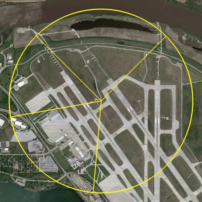
Table 1. Example Joint Frequency Table of wind direction and wind speed
 Dir \ Spd ≤ 3knots ≤ 6 knots ≤ 10 knots ≤ 16 knots ≤ 21 knots > 21 knots Total
0.0 0.11% 0.53% 1.37% 0.83% 0.12% 0.03% 2.98%
10.0 0.08% 0.50% 0.99% 0.47% 0.05% 0.01% 2.10%
20.0 0.06% 0.41% 1.04% 0.59% 0.17% 0.08% 2.34%
30.0 0.09% 0.31% 0.91% 0.46% 0.13% 0.07% 1.96%
40.0 0.09% 0.35% 0.79% 0.47% 0.09% 0.02% 1.81%
50.0 0.07% 0.30% 0.61% 0.30% 0.08% 0.03% 1.40%
60.0 0.08% 0.22% 0.54% 0.25% 0.07% 0.03% 1.19%
70.0 0.05% 0.28% 0.50% 0.24% 0.05% 0.02% 1.14%
80.0 0.05% 0.23% 0.51% 0.23% 0.06% 0.01% 1.08%
90.0 0.05% 0.23% 0.58% 0.22% 0.05% 0.03% 1.16%
100.0 0.05% 0.21% 0.60% 0.26% 0.05% 0.01% 1.19%
110.0 0.05% 0.30% 0.67% 0.46% 0.06% 0.01% 1.56%
120.0 0.08% 0.34% 0.97% 0.48% 0.10% 0.04% 2.01%
130.0 0.12% 0.63% 1.54% 0.76% 0.17% 0.02% 3.25%
140.0 0.10% 0.56% 1.55% 0.96% 0.17% 0.04% 3.38%
150.0 0.11% 0.42% 1.74% 1.48% 0.28% 0.04% 4.06%
160.0 0.08% 0.32% 1.61% 1.73% 0.41% 0.06% 4.21%
170.0 0.08% 0.29% 1.61% 1.71% 0.42% 0.08% 4.19%
180.0 0.07% 0.37% 1.95% 1.82% 0.55% 0.17% 4.93%
190.0 0.09% 0.40% 1.67% 1.48% 0.45% 0.16% 4.24%
200.0 0.08% 0.37% 1.41% 0.93% 0.34% 0.08% 3.22%
210.0 0.06% 0.33% 1.29% 0.69% 0.16% 0.02% 2.54%
220.0 0.08% 0.29% 0.94% 0.57% 0.15% 0.04% 2.07%
230.0 0.07% 0.27% 0.97% 0.53% 0.09% 0.03% 1.96%
240.0 0.07% 0.23% 0.76% 0.30% 0.10% 0.04% 1.49%
250.0 0.06% 0.27% 0.68% 0.29% 0.07% 0.03% 1.41%
260.0 0.05% 0.25% 0.77% 0.33% 0.10% 0.08% 1.57%
270.0 0.03% 0.23% 0.89% 0.50% 0.13% 0.07% 1.84%
280.0 0.05% 0.23% 0.90% 0.59% 0.21% 0.08% 2.07%
290.0 0.05% 0.35% 1.03% 0.65% 0.22% 0.08% 2.38%
300.0 0.07% 0.42% 0.86% 0.59% 0.17% 0.05% 2.16%
310.0 0.09% 0.44% 1.40% 0.93% 0.36% 0.13% 3.35%
320.0 0.08% 0.60% 1.68% 1.14% 0.49% 0.16% 4.14%
330.0 0.05% 0.42% 1.56% 1.52% 0.75% 0.31% 4.62%
340.0 0.10% 0.50% 1.27% 1.17% 0.36% 0.10% 3.49%
350.0 0.11% 0.50% 1.36% 1.12% 0.28% 0.07% 3.45%
Total 2.65% 12.90% 39.52% 27.04% 7.48% 2.33% 91.92%
Calms 5.52%
Missing 2.56%
Total 100%

 7

For example, the wind roses from Charles City, IA (Figure 1) and Oelwein, IA (Figure 2) are very similar, and have a
correlation coefficient of 0.933.

 Figure 1. Wind Rose for Charles City, IA (KCCY) Figure 2. Wind Rose for Oelwein, IA (KOLZ)

On the other hand, the wind roses from Omaha, NE (Figure 3) and Boscobel, WI (Figure 4) are very dissimilar, and have a
correlation coefficient of 0.036.

 Figure 3. Wind Rose for Omaha, NE (KOMA) Figure 4. Wind Rose for Boscobel, WI (KOVS)

Generally, correlation coefficients of 0.9 or higher were observed when two wind roses were very similar and 0.8 or
higher when only mild differences were observed between two wind roses. The differences between wind roses became
more evident when the correlation coefficient was less than 0.8. For these reasons, 0.9 and 0.8 were chosen as
thresholds to indicate ideal and good similarity, respectively. These criteria were then used as a baseline for the
remainder of this analysis.

Determining the Effect of Separation Distance on Representivity
To account for spatial proximity, a distance-weighted scaling factor was applied to the wind correlation coefficient.
Doing so serves to account for the potential differences caused purely by the distance between two points in the
overlying mesoscale conditions, such as temperature, pressure, and cloud cover. A sensitivity analysis was conducted to
evaluate the effect of separation distance on meteorological variables. This analysis was completed using the 2005-2009
dataset which was the most recent readily available dataset. This analysis is still valid therefore it was no redone with
the 2010-2014 dataset.

 8

Nineteen ASOS sites across Iowa and surrounding states were used: Ames, Burlington, Cedar Rapids, Davenport, Des
Moines, Dubuque, Estherville, Iowa City, La Crosse (WI), Lamoni, Marshalltown, Mason City, Moline (IL), Omaha (NE),
Ottumwa, Sioux City, Sioux Falls (SD), Spencer and Waterloo. Hourly temperature, pressure and cloud cover
observations from the existing 2005-2009 dataset was used. Using these data allowed the sensitivity analysis to be
conducted prior to the processing of the 2015-2019 data for which the results would be used. Temperature, pressure
and cloud cover were chosen because those are the primary meteorological variables used in dispersion modeling (other
than wind speed and direction). Wind data was not included because it can be affected by localized terrain influences,
and is already considered in the wind correlation analysis described above.

First, the distance between each pair of meteorological sites was determined. Next, the correlation between the hourly
data at each pair of meteorological sites was calculated for each of the three variables (temperature, pressure, and
cloud cover). Finally, the correlations of the three variables for each pair of meteorological sites were averaged, resulting
in a single correlation between each pair of sites. Figure 5 shows how the average correlation varies with distance.

 Figure 5. Average Correlation for All Nineteen Meteorological Sites

As expected, the average correlation decreases with distance. Unexpectedly, there were several site correlations (circled
above) that appeared to be outliers. After further investigating the outliers, it was revealed that each included Des
Moines as one of the sites. To determine what was causing the discrepancy each variable was plotted individually as
shown in Figure 6.

 9

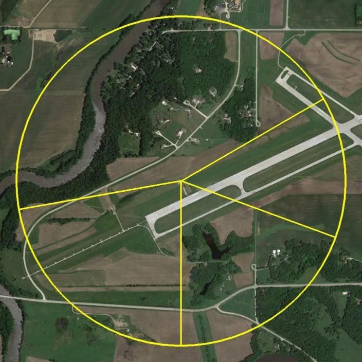
Figure 6. Temperature, Pressure and Cloud Cover Correlation

The temperature and pressure correlation are plotted on the left and the cloud cover correlation is plotted on the right.
The cloud cover has the same distinct group of outliers as Figure 5.

The Des Moines cloud cover data were analyzed to determine the source of the correlation anomaly. AERMET breaks
cloud cover into tenths. The numbers are based on sky coverage; no cloud coverage (0) – total cloud coverage (10).
Table 2 shows the hourly breakdown of the Des Moines cloud cover from 2005-2009.

 Table 2. Des Moines Cloud Cover Count
 Sky Coverage (tenths) Number of Hours
 0 9,580
 1 0
 2 28
 3 6,077
 4 19
 5 4,303
 6 0
 7 35
 8 1,135
 9 5,404
 10 17,243

The same method was performed for the Ames and La Crosse (WI) stations. Ames was analyzed because it is the closest
site to Des Moines and therefore should have the most similar cloud cover. La Crosse (WI) was analyzed because it had
the lowest cloud cover correlation with Des Moines. The hourly cloud cover breakdown for both sites is listed in Table 3.

 10

Table 3. Ames and La Crosse, WI Cloud Cover Count
 Sky Coverage (tenths) Number of Hours - Ames Number of Hours - La Crosse
 0 22,573 22,058
 1 0 0
 2 0 5
 3 4,183 2,192
 4 0 6
 5 1,966 1,539
 6 0 0
 7 0 5
 8 53 0
 9 3,209 3,017
 10 11,840 15,002

In comparing the Des Moines breakdown to the other two sites it is clear that Des Moines is reporting greater numbers
of cloudy hours and fewer clear hours then Ames and La Crosse (WI). The Des Moines National Weather Service Office
(19) was contacted and provided an explanation for this observation. The Des Moines International Airport records
cloud cover above 12,000 feet due to its classification and contract with the Federal Aviation Administration (FAA). The
Des Moines National Weather Service confirmed that all of the other 18 meteorological sites used in this representivity
analysis do not report clouds above 12,000 feet. If no clouds are detected below 12,000 feet the hour is reported as
clear, which translates into a zero for cloud cover, even if higher-altitude clouds were present. To ensure that this was
indeed the reason for the group of outliers, the Des Moines cloud cover data was adjusted by changing all non-zero
cloud cover observations above 12,000 feet into zeros. The revised data was then re-processed through AERMET. Table
4 is the Des Moines cloud cover results with clear skies above 12,000 feet.

 Table 4. Des Moines Clear Skies above 12,000 Feet
 Sky Coverage (tenths) Number of Hours
 0 17,604
 1 0
 2 28
 3 6,076
 4 19
 5 4,300
 6 0
 7 11
 8 607
 9 1,976
 10 13,203

Figure 7 and Figure 8 shows how the cloud cover correlation changed with the removal of cloudy skies above 12,000 feet
in the Des Moines meteorological data.

 11

Figure 7. Original Cloud Cover Correlation

 Figure 8. Corrected Cloud Cover Correlation

Replacing cloudy skies with sunny skies for cloud cover above 12,000 feet removed the outlier group; concluding that
this discrepancy in ASOS reporting is the cause. Using the adjusted cloud cover correlation, the average correlation for
all sites is re-plotted in Figure 9.

 12

Figure 9. Adjusted Averaged Correlation

However, to find a distance cutoff the Des Moines data was excluded due to the discrepancy stated above. Since EPA
does not have guidance on this reporting difference, the cloud cover above 12,000 feet was not removed from the Des
Moines data. As shown previously in Figure 5 this difference does affect the overall correlation and in order to get the
correct distance cutoff the Des Moines data was removed (Figure 10).

 Figure 10. Average Correlation without Des Moines Data

Removing the Des Moines data eliminates the outlier group and produces near perfect correlation between distance
and cloud cover. In this analysis a 0.8 correlation is considered the minimum good fit correlation. Using the best fit
equation and substituting 0.8 for “y”, it is determined that a meteorological site could be separated from the application
site by up to 284 km before this correlation coefficient falls below 0.8.

The relationship between correlation and separation distance was then converted into a function that could be used to
apply a distance-weighted scaling factor to each wind correlation coefficient. This function was developed in such a way
that the resulting scaling factor would not modify the wind correlation coefficient when there was no separation error,
 13

and would reduce the wind correlation coefficient between two perfectly correlated sites that are separated by up to
284 km to the minimum correlation considered a good fit (0.8).

This was accomplished using Equation 1:

 Equation 1

 = 1 − ( ∗ )

Where: Q = Distance-weighted scaling factor
 M= Mesoscale coefficient
 D= Distance (km)

The mesoscale coefficient is derived from the data in Figure 10 using Equation 2:

 Equation 2

 (1 − )
 =
 
Where: RMin = Minimum desired correlation
 DMax = Maximum distance (km) at which RMIN is met

Substituting 0.8 for RMIN, and 284 km for DMAX results in M = 0.000704225. Thus, Equation 1 becomes:

 Equation 3

 = 1 − (0.000704225 ∗ )

Applying Equation 3 to the correlation coefficients of every pair of wind roses results in a distance-weighted correlation
coefficient. Using two perfectly correlated (correlation coefficient = 1.0) wind roses as an example:

 • If the wind roses are from collocated sites (D = 0), Equation 3 becomes:

 Q = 1 – (0.000704225 *0) = 1 – 0 = 1.0

 The correlation coefficient (1.0) for the two identical wind roses from collocated sites would be multiplied by 1,
 and therefore remain perfectly correlated (1.0).

 • If the wind roses are from sites separated by 284 kilometers (D = 284), Equation 3 becomes:

 Q = 1 – (0.000704225 * 284) ≈ 1 – 0.2 = 0.8

 The correlation coefficient (1.0) for the two identical wind roses from sites separated by a distance of 284
 kilometers would be multiplied by 0.8, and therefore be reduced to the minimum correlation previously defined
 as being a good fit (0.8).

A distance-weighting factor was calculated as described above for every possible combination of measurement sites,
and then applied to the corresponding correlation coefficients for those combinations.

 14

Selection of AERMOD Meteorological Sites
For various reasons, only a portion of the 93 sites for which wind roses were created could be used to process data for
use in AERMOD. The following factors were considered when determining which of the sites would be further analyzed
for use in the model:
 • Existence of concurrent 1-minute data.
 • Fulfillment of the 90% data completeness criterion.
 • Correlation of the wind roses.

Of the 93 sites, 21 were chosen for processing (see Table 5). These include three sites not used in the 2010-2014 dataset
(Blair, NE; Decorah, IA; and Fort Dodge, IA). The addition of these sites significantly improves the coverage of
representative meteorological data. One site from the 2010-2014 dataset has been removed (La Crosse, WI). Previously,
this site was used in the upper Mississippi River Valley. The DNR has since determined that this site is not representative
of many sections of the river valley and has decided not to process it for use in the model. All but three of the chosen
sites have 1-minute data available. For those three sites, sub-hourly ASOS wind data was obtained from the Iowa
Environmental Mesonet (IEM). This data was processed manually to replicate the average wind conditions for each hour
that would have been produced had 1-minute data been available.

The data for Decorah did not meet the 90% completeness criterion during the third quarter of 2015 (~82%) and the third
quarter of 2016 (~86%). The EPA Region 7 office approved the use of this data set because it is more representative of
the far northeast corner of the state than any of the alternatives that meet the 90% criterion. The expectation being that
the Iowa DNR would fill in the missing data using sub-hourly data from the Decorah site obtained from the IEM.

 Table 5. The 21 Surface Stations Used to Process Data for AERMOD
 Station Call Sign
 Ames, IA KAMW
 Blair, NE KBTA
 Burlington, IA KBRL
 Cedar Rapids, IA KCID
 Davenport, IA KDVN
 Decorah, IA KDEH
 Des Moines, IA KDSM
 Dubuque, IA KDBQ
 Estherville, IA KEST
 Fort Dodge, IA KFOD
 Iowa City, IA KIOW
 Lamoni, IA KLWD
 Marshalltown, IA KMIW
 Mason City, IA KMCW
 Moline, IL KMLI
 Omaha, NE KOMA
 Ottumwa, IA KOTM
 Sioux City, IA KSUX
 Sioux Falls, SD KFSD
 Spencer, IA KSPW
 Waterloo, IA KALO

 15

Determination of the Areas Represented by Each Meteorological Site
The final step in the process was to use the distance-weighted correlation coefficients to determine those portions of
the state for which each meteorological station listed in Table 5 is representative. Traditionally, county borders have
been used as convenient boundaries that can be easily referenced to determine which meteorological dataset to use for
various areas of the state. However, research conducted by the Iowa DNR shows that there are areas of the state where
meteorological representivity may vary within a county, specifically: areas affected by portions of the Missouri or
Mississippi River valleys. Figure 3 provides an example of such an area.

The Omaha, NE meteorological measurement site is located within the Missouri River valley. Its wind rose is most
correlated with the wind rose from Tekamah, NE, which is also located in the Missouri River valley approximately 50 km
N-NW of the Omaha, NE site, but it is far less correlated with the wind rose from Council Bluffs, IA, which is located only
8 km to the east of the Omaha, NE site, but is situated on the bluff above the Missouri River valley. This is an obvious
indication that the Missouri River valley effects the overlying mesoscale flow along this stretch of the river. Similar
effects can be seen along the remainder of the Missouri River valley bordering Iowa, and along the stretch of the
Mississippi River valley upstream from Moline, IL.

In order to determine if a meteorological site is influenced by a river valley, an analysis was performed to find an
objective method for determining when a site is influenced by river valley terrain. The wind patterns are quantified using
a diurnal temperature in order to calculate an index value for every wind direction. An index value of 0.0023 was used as
a cutoff. Only sites with a terrain index value above this cutoff are considered to be influenced by river valley terrain.
This index value cutoff corresponds to a valley depth of 60 meters (or greater). The 60-meter depth threshold is used to
identify the portions of the Mississippi and Missouri River valleys that are influenced by river valley terrain. Counties in
Iowa affected by river valley wind channeling were subdivided into a portion of the county represented by a valley site
and the remaining portion represented by a non-valley site.

In order to determine which areas of the state would be represented by each meteorological site the distance-weighted
correlation coefficient data were input into Golden Software’s Surfer program (20). Using this program, a grid was
placed across the entire state with grid nodes in the center of each county. Surfer was then used to calculate the
distance-weighted correlation coefficient at each grid point for each meteorological site listed in Table 5.

In most cases, the meteorological site with the highest distance-weighted correlation coefficient at each grid point was
then assigned as the most representative site for that county. In some cases, there were two or more meteorological
sites that were estimated to be similarly representative. When this occurred the chosen site was often the location that
would prevent a meteorological site from representing multiple non-contiguous areas of the state. The resulting
representative areas are depicted in Figure 11.

 16

Figure 11. Representative Areas for the 2015 – 2019 AERMOD Meteorological Dataset

For those counties that were subdivided into valley and non-valley areas, the edge of the flood plain defines the border
of the corresponding representative area. For areas on the map where the county is subdivided, a modeling analysis
with sources located within the floodplain would use the meteorological data from the subdivision representing the
river valley in that area, and an analysis with sources located anywhere other than the floodplain would use the
meteorological data from the subdivision representing the remainder of the county. The abrupt increase in elevation
adjacent to the floodplain used to define the boundary can be determined by inspecting topographic maps of the area.

A major change from the 2010-2014 dataset is the removal of the La Crosse, WI data for the Upper Mississippi River
Valley. The meteorological conditions in this stretch of the river are highly influenced by the orientation of the valley at
any specific location, as can be seen in the wind data for La Crosse, WI and Prairie Du Chien, WI. As such, the DNR has
determined that the La Crosse, WI data is not representative of many sections of the valley. In addition, there are only a
small number of facilities located in this section of the valley. For these reasons the DNR has decided to treat projects in
portions of the Mississippi River Valley north of Clinton County on a case-by-case basis. Applicants located in this
section of the Mississippi River Valley should contact the DNR for guidance prior to conducting modeling.1

In Muscatine County, the two highest-correlated sites were Iowa City (0.91) and Davenport (0.88). The majority of
modeling conducted in the county occurs in the PM2.5 and SO2 SIP areas (generally located on the southeastern edge of
the county). When the distance-weighted correlation coefficients are calculated based on the location of the SIP areas

1
 In some cases, it may be appropriate for applicants in this area of the State to conservatively estimate model results by using a
large sample of less representative data. The DNR evaluated model results for multiple facilities located within the upper Mississippi
River valley using data from all 2010-2014 meteorological data sites. The highest ranked results were captured using data from a
combination meteorological sites nearest to the upper Mississippi River valley (excluding La Crosse, WI). Therefore, future modeling
projects that are evaluated using all seven sites in the 2015-2019 data set nearest to the valley (KALO, KCID, KDBQ, KDEH, KDVN,
KIOW, and KMLI) would be expected to produce a conservative estimate. Use of the meteorological data in this way should not be
confused with “representivity.” If an approach like this is approved for a project it will be considered a conservative estimate and not
a representative result. Any conservative approach may result in permit limits that are more stringent than would otherwise be
required if representative data were used. However, there may be projects where a conservative estimate is acceptable to the
applicant and thus the DNR is providing this as one possible approach to conducting a modeling analysis in this area.
 17

they become 0.89 for both the Iowa City and Davenport data. In this case, Davenport was chosen as the representative
site because a thorough representivity analysis has already been conducted as part of several modeling analyses
conducted in Muscatine.

The distance-weighted correlation coefficient of the chosen representative site for each area is depicted in Figure 12.
Areas where the distance-weighted correlation is 0.9 or greater are shaded in blue. Areas where the distance-weighted
correlation is 0.8 or greater, but less than 0.9 are shaded in green. Areas where the distance weighted correlation is less
than 0.8 are not shaded. The red dots represent the valley-based meteorological stations used to represent the portions
of the Missouri and Mississippi River valleys where the wind patterns are significantly affected by those valleys, and the
black dots represent the remaining meteorological stations.

 Figure 12. Distance-Weighted Correlation of Chosen Representative Sites

As shown by the map, approximately 98% of the state is represented by a meteorological station that is either ideally or
well correlated (distance-weighted correlation coefficient greater than 0.9 or 0.8, respectively). Only about 2% is
represented by less-correlated meteorological stations. This is mainly due to a lack of data in these areas of the state.

The representativeness of the upper air data was determined purely based on spatial proximity because the
measurements are taken above the surface where local geographic features and land cover do not have an effect. The
two nearest upper air sites are Omaha, NE and Davenport, IA. These data were applied to roughly the half of the state
each is nearest to. The surface data from KAMW, KBTA, KDSM, KEST, KFOD, KFSD, KLWD, KMCW, KOMA, KSPW, and
KSUX were paired with the Omaha upper air data. The surface data from KALO, KBRL, KCID, KDBQ, KDEH, KDVN, KIOW,
KMIW, KMLI, and KOTM were paired with the Davenport upper air data.

It should be noted that this representivity analysis is intended to provide a guide for general representivity only. The
meteorological data assigned to each area of the state by this analysis is only representative to the extent that no local
features would significantly alter the meteorological conditions in the area where it is to be applied.

 18

Filling Missing Surface Data
Surface data were only filled for the 21 meteorological stations chosen during the representivity analysis (listed in Table
5). An Excel spreadsheet consisting of a series of embedded programs was used to fill all missing surface data. This
program was developed in-house, and is called AERFILL.

The AERFILL program fills missing data using the recommendations in “Procedures for Substituting Values for Missing
NWS Meteorological Data for Use in Regulatory Air Quality Models” by Dennis Atkinson and Russell F. Lee (21), and
quality assures (QA) the results following the recommendations in EPA’s “Meteorological Monitoring Guidance for
Regulatory Modeling Applications” document (22). Much of the data filling was performed automatically by AERFILL.
Longer, or more problematic gaps, and most quality assurance related decisions, were addressed manually.

The data were filled using various techniques, ranging from simple interpolations or persistence, to complicated spatially
and temporally-weighted averages based on surrounding meteorological stations. In many instances, the data were
filled based on the application of meteorological principles and techniques. Comments were included in the file
indicating what method was used (one comment for each time the data were edited). The results of the representivity
analysis were used to determine which alternate source of data was most likely to provide the best fit. Generally, data
from the most representative station was available and was determined to be appropriate. If the data from the most
representative neighboring station did not appear to fit or was also missing, the data from the next most representative
station was evaluated. This process continued down the hierarchy of most representative stations until acceptable data
was found.

After the data were completely filled, a QA procedure was executed. All QA flags were reviewed for relevance and
importance. In most cases the flags did not signify inaccurate data, just extremes in the data due to the applicable
weather conditions. The more questionable data were cross-checked with other sources of information including one or
more of the following:
 • The raw ISH data for the station in question.
 • ASOS data from the IEM (23) for the station in question.
 • The raw ISH data for neighboring stations.
 • ASOS data from the IEM for neighboring stations.
 • AWOS/RWIS (Road Weather Information System) data from the IEM for neighboring stations.
 • Weather Underground Past Data
 • Iowa Mesonet Time Machine

If the data appeared to be meteorologically impossible or improbable, and could not be correlated with the cross-
referenced sources, it was adjusted using data-filling schemes similar to those used to fill missing data. An example of
this would be if the station pressure for five consecutive hours was 980.0 mb, 980.1 mb, 915.5 mb, 980.3 mb and 980.5
mb. In this case, it is clear that the third value is invalid, and would have been replaced with a value of 980.2 mb.

If the data seemed to be meteorologically reasonable, or correlated with the cross-referenced sources, it was not
modified. An example of this would be the occurrence of a cold front. A cold front could cause a rapid shift in pressure,
temperature, wind and cloud cover, all of which would be flagged by AERFILL’s QA routine, even though the data were
valid.

After the QA was complete the data were exported from AERFILL in the format of an AERMET QA input file, ready to be
merged with the 1-minute and upper air data.

 19

Filling Missing Upper Air Data
Missing upper air data can cause an under-prediction bias in AERMOD. This effect, and procedures for filling missing
upper air data, are outlined in the document “A Method for Filling AERMET Upper Air Data” (24). The procedures
described in that document were used to fill the missing data.

The raw data from four sites (Davenport, IA; Lincoln, IL; Minneapolis, MN; and Omaha, NE) were processed using
AERMET. The output from AERMET was then imported into Excel and sorted in order to create a list of available morning
soundings at each location. Evening soundings are not currently used by AERMET, and were therefore not evaluated.
The morning sounding inventory is summarized in Table 6.

 Table 6. Morning Sounding Inventory
 Station Available Morning Soundings Percentage
 Davenport, IA 1,810 99.1%
 Lincoln, IL 1,818 99.6%
 Minneapolis, MN 1,801 98.6%
 Omaha, NE 1,807 99.0%

Using this information, the raw data were edited to fill in the missing morning soundings. Only data from the two
nearest sites (Davenport and Omaha) were used to process data for AERMOD, so only those data were filled. In cases
where the data from only one of these locations was missing, the corresponding sounding from the other location was
used to fill in the gap. There were no instances where the sounding was missing from both Davenport and Omaha.

These edited data were then reprocessed with AERMET to produce the files necessary to be merged with the surface
and 1-minute data.

 20

1-Minute Data (AERMINUTE)
The latest version of AERMINUTE available at the time of processing (dated 15272) was used to process the 1-minute
data for each of the 18 meteorological stations processed for use in AERMOD. The 1-minute wind data was obtained
from the NCDC’s online ftp directory (4) in the 6405 format, which is compatible with the AERMINUTE program. The
downloaded data consists of text files; each text file contains data for one station-month.

The 1-minute wind data consist of a running 2-minute average that are reported every minute at each ASOS station. The
archived 1-minute wind data contained in the downloaded text files from the NCDC were used to calculate the hourly
average wind speed and direction, which could then be used to supplement the standard archive of hourly observed
winds in the surface data – reducing the number of calms, variable winds, and missing data.

The AERMINUTE preprocessor requires the user to indicate the start and end month and year of the data being
processed as well as whether or not the station is part of the Ice Free Winds (IFW) group. The IFW group refers to ASOS
sites that use sonic anemometers instead of cup and vane anemometers to measure winds. If the station is part of the
IFW group during the data period being processed by AERMINUTE, then the IFW installation date must be entered into
the program. The website indicated in section 3.1.2 of the AERMINUTE user guide (25) was used to determine if the
stations were part of the IFW group and their respective installation dates.

AERMINUTE gives an option to include data files of standard NWS observations in order to compare the non-quality
controlled 1-minute winds against the quality controlled standard observations. The raw ISH data for each of the
eighteen stations being processed was included in the AERMINUTE input file for comparison with each of these stations
1–minute raw data files.

The combination of the above described data was processed by AERMINUTE to produce the necessary output file for
merging with the filled and edited surface and upper air data.

Three sites (Blair, NE (KBTA); Decorah (KDEH), and Fort Dodge (KFOD)) do not have 1-minute data available. The
methods used by AERMINUTE to determine the hourly average wind speed and direction was reproduced within a series
of spreadsheets. Sub-hourly data from the IEM was then input into these spreadsheets and were used to replicate the
average wind conditions for each hour that would have been produced had 1-minute data been available. Also, January
of 2018 for the Omaha, NE (KOMA) site did not have 1-minute data available, therefore sub-hourly data was used.

Even after processing the sub-hourly data for KBTA, KDEH and KFOD these sites contained far more calms than any of
the other data sets. The Decorah data contained 9% calms, Fort Dodge 6%, and Blair 3%. For comparison, after
processing the 1-minute data, the average amount of calms in all of the other data sets was 0.4% with the highest being
1%. Initial sensitivity tests indicated that the higher number of calms at the sites without 1-minute data would create a
bias towards low predictions.

Based on this information it seemed prudent to decrease the number of calms in these three datasets. Each calm hour
within one hour of a non-calm record at these three sites was filled using a wind speed of 1 m/s and the same wind
direction as the nearest non-calm hour. This method of filling calms is the same that was used in the DNR’s 2000-2004
meteorological data sets (prior to the availability of 1-minute data). After this was accomplished the average percentage
of calms for these three sites was reduced from 6% to 2%, with the highest percentage for any one year being 3%
(Decorah). This is still higher than the sites with 1-minute data, but updated sensitivity tests show that this change
eliminates the bias towards low predictions.

The method used to fill calms is similar to the way calms used to be treated before calms processing routines were
developed. Before calms processing, a “calm” was defined as an hour with a wind speed of 1.0 m/s and a wind direction
that was equal to the previous hour. This method produced conservative estimates and avoided division by zero in the
dispersion equations of earlier models. Since then, calms processing routines have been built into the models to modify
the averages during periods in which calms are present. Filling all calms that occur within one hour of a non-calm hour is
a hybrid of the two techniques. In other words, calms are filled via persistence to a certain extent, but left intact for the
calms processing routines to handle during longer periods.
 21

Land Use Analysis
The latest version of AERSURFACE (dated 19191) was used to conduct the land use analysis for each meteorological site.
This version of AERSURFACE uses the 2016 land use, tree canopy and impervious surfaces data. While the data were
processed in accordance with the guidance available in the AERSURFACE user guide (9), two additional levels of detail
were added to this stage of processing. These include refinements to the snow cover and surface moisture condition
estimates.

Snow Cover and Surface Moisture Conditions
The AERSURFACE preprocessor requires the user to indicate whether or not the site experiences continuous snow cover
during the winter months, and if the area experienced below normal, above normal or average surface moisture
conditions.

Daily snow cover maps from NCDC were analyzed for the entire 2015-2019 period (26). An example of a daily snow
cover map is depicted in Figure 13.

 Figure 13. Example Daily Snow Cover Map

For each day of the period, a determination of whether or not snow cover was present at each meteorological station
was made based on visual estimates of the proximity of snow cover shown on the maps to the stations being processed.
These data were then combined to determine which months of the year should be considered as having continuous
snow cover at each station. Continuous snow cover was assumed for each month during which there was snow cover
during at least half of the days in that month at that site (marked by the letter “X” in Tables Table 7-Table 11).

To determine the relative surface moisture conditions during each month of the period, monthly climatological
divisional precipitation rank maps were analyzed (27). An example of a monthly climatological divisional precipitation
rank map is depicted in Figure 14.

 22

Figure 14. Example Monthly Climatological Divisional Precipitation Rank Map

Areas shown as “Record Driest” or “Much Below Normal” were categorized as being dry. Areas shown as “Below
Normal”, “Near Normal” or “Above Normal” were categorized as average. Areas shown as “Much Above Normal” or
“Record Wettest” were categorized as wet. These categories approximate the guidance in section 2.2 of the
AERSURFACE user guide (9):

 The surface moisture condition can be determined by comparing precipitation for the period of data to
 be processed to the 30-year climatological record, selecting “wet” conditions if precipitation is in the
 upper 30th-percentile, “dry” conditions if precipitation is in the lower 30th-percentile, and “average”
 conditions if precipitation is in the middle 40th-percentile.

Dry conditions are represented in Tables Table 7-Table 11 with orange-shaded cells, wet conditions are represented with
blue-shaded cells and average conditions are not shaded.

 23

Table 7. Snow Cover and Moisture Conditions – 2015

 September

 November

 December
 February

 October
 January

 August
 March

 April

 June
 May

 July
 Station

KALO (Waterloo) X X
KAMW (Ames) X
KBRL (Burlington) X X
KBTA (Blair NE) X X
KCID (Cedar Rapids) X X
KDBQ (Dubuque) X X
KDEH (Decorah) X X X
KDSM (Des Moines) X
KDVN (Davenport) X X
KEST (Estherville) X X X
KFOD (Fort Dodge) X X
KFSD (Sioux Falls SD) X X X
KIOW (Iowa City) X X
KLWD (Lamoni) X
KMCW (Mason City) X X
KMIW (Marshalltown) X X
KMLI (Moline IL) X X
KOMA (Omaha NE) X X
KOTM (Ottumwa) X
KSPW (Spencer) X X X
KSUX (City City) X X X

 Table 8. Snow Cover and Moisture Conditions - 2016
 September

 November

 December
 February

 October
 January

 August
 March

 April

 June
 May

 July

 Station

KALO (Waterloo) X X X
KAMW (Ames) X X X
KBRL (Burlington) X
KBTA (Blair NE) X X
KCID (Cedar Rapids) X X X
KDBQ (Dubuque) X X X
KDEH (Decorah) X X X
KDSM (Des Moines) X X
KDVN (Davenport) X X
KEST (Estherville) X X X
KFOD (Fort Dodge) X X X
KFSD (Sioux Falls SD) X X X

 24

September

 November

 December
 February

 October
 January

 August
 March

 April

 June
 May

 July
 Station

KIOW (Iowa City) X X X
KLWD (Lamoni) X X
KMCW (Mason City) X X X
KMIW (Marshalltown) X X X
KMLI (Moline IL) X X X
KOMA (Omaha NE) X X
KOTM (Ottumwa) X X
KSPW (Spencer) X X X
KSUX (Sioux City) X X

 Table 9. Snow Cover and Moisture Conditions – 2017

 September

 November

 December
 February

 October
 January

 August
 March

 April

 June
 May

 July
 Station

KALO (Waterloo) X X
KAMW (Ames) X
KBRL (Burlington)
KBTA (Blair NE)
KCID (Cedar Rapids)
KDBQ (Dubuque) X
KDEH (Decorah) X X
KDSM (Des Moines)
KDVN (Davenport)
KEST (Estherville) X X
KFOD (Fort Dodge) X
KFSD (Sioux Falls SD) X X
KIOW (Iowa City)
KLWD (Lamoni)
KMCW (Mason City) X X
KMIW (Marshalltown)
KMLI (Moline IL)
KOMA (Omaha NE)
KOTM (Ottumwa)
KSPW (Spencer) X X X
KSUX (Sioux City) X

 25

Table 10. Snow Cover and Moisture Conditions – 2018

 September

 November

 December
 February

 October
 January

 August
 March

 April

 June
 May

 July
 Station

KALO (Waterloo) X X
KAMW (Ames) X X
KBRL (Burlington) X
KBTA (Blair NE) X X X
KCID (Cedar Rapids) X X
KDBQ (Dubuque) X X
KDEH (Decorah) X X X X
KDSM (Des Moines) X X
KDVN (Davenport) X X
KEST (Estherville) X X X X X
KFOD (Fort Dodge) X X X
KFSD (Sioux Falls SD) X X X X X
KIOW (Iowa City) X
KLWD (Lamoni) X
KMCW(Mason City) X X X X X
KMIW (Marshalltown) X X
KMLI (Moline IL) X X
KOMA (Omaha NE) X X X
KOTM (Ottumwa) X
KSPW (Spencer) X X X X X
KSUX (Sioux City) X X X X

 Table 11. Snow Cover and Moisture Conditions – 2019
 September

 November

 December
 February

 October
 January

 August
 March

 April

 June
 May

 July

 Station

KALO (Waterloo) X X
KAMW (Ames) X X
KBRL (Burlington) X X
KBTA (Blair NE) X X
KCID (Cedar Rapids) X X
KDBQ (Dubuque) X X
KDEH (Decorah) X X X X
KDSM (Des Moines) X X
KDVN (Davenport) X X
KEST (Estherville) X X
KFOD (Fort Dodge) X X
KFSD (Sioux Falls SD) X X X X

 26

September

 November

 December
 February

 October
 January

 August
 March

 April

 June
 May

 July
 Station

 KIOW (Iowa City) X X
 KLWD (Lamoni) X X
 KMCW (Mason City) X X X X
 KMIW (Marshalltown) X X
 KMLI (Moline IL) X X
 KOMA (Omaha NE) X X
 KOTM (Ottumwa) X X
 KSPW (Spencer) X X X X
 KSUX (Sioux City) X X

Land Cover Data
The National Land Cover Dataset from 2016 (NLCD92) was chosen for this analysis because the AERSURFACE
preprocessor had been updated to use the 2016 land cover data, the most recent available. The land cover data were
obtained from the Multi-Resolution Land Characteristics Consortium (7) in GEOTIFF format. The classifications included
in this data are summarized in Figure 15.

 Figure 15. 2016 National Land Cover Dataset Classification Summary

Processing Data in AERSURFACE
The first step in processing the land use data in AERSURFACE is to divide the area around each site into one or more
sectors. The sectors were determined by examining the land use surrounding the site in all directions. Sites with little to
no change in land use in any direction were processed using a single sector that encompassed the entire 360 degrees.
Otherwise, areas with similar land use were grouped and the angular direction of each area was determined. For
example, a site with a residential area along the eastern half and crops along the western half would be divided into two
sectors with the boundaries of each at 0 degree and 180 degrees. A secondary consideration in defining the sectors was
the type of “Developed” land cover in each sector. Each of the sites is located at an airport. Sectors that encompass
portions of the airport need to be treated differently because the “Developed” land use categories do not distinguish
between runways (low surface roughness) and areas with buildings (high surface roughness). AERSURFACE distinguishes
 27

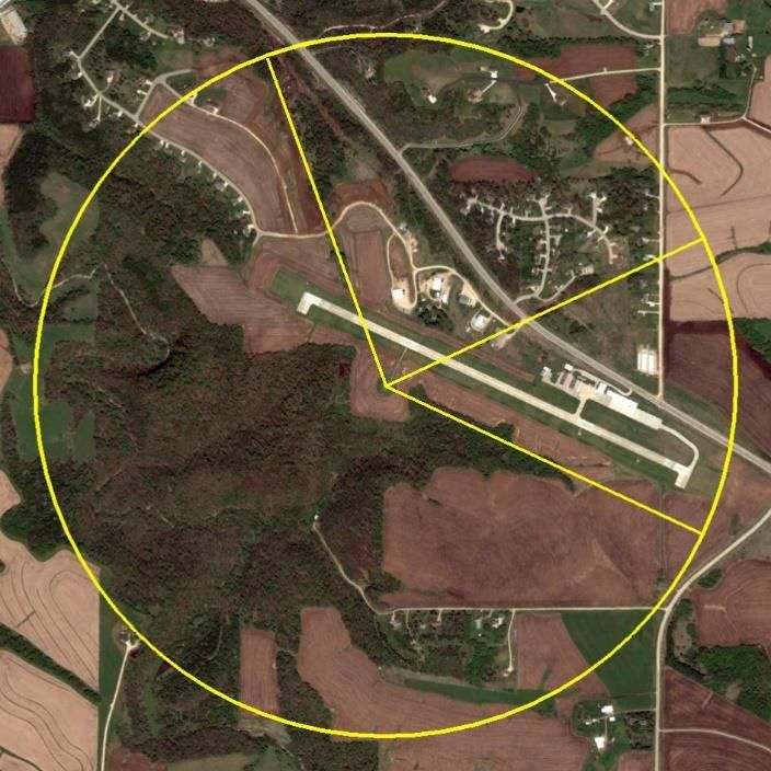
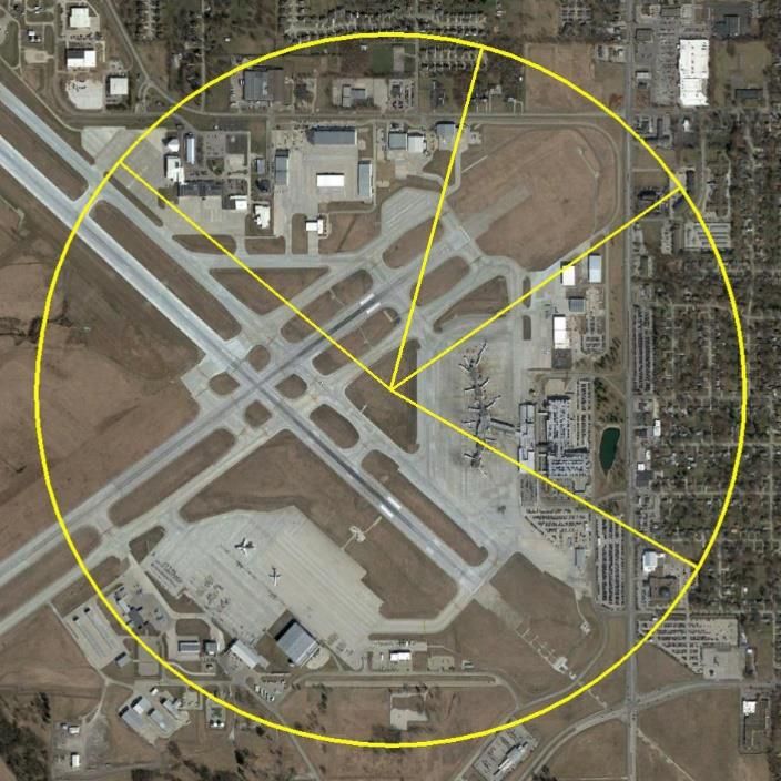
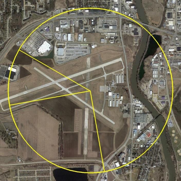
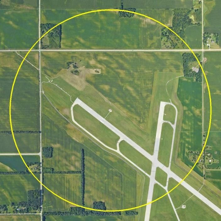
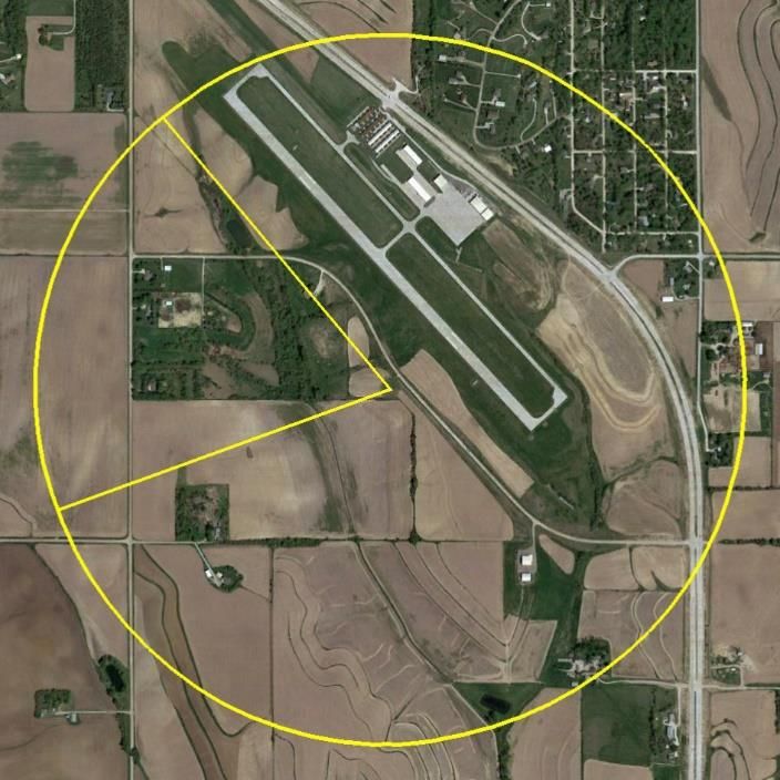
between these different land uses, but it requires the user to input what type of area each sector is. In order to account
for this it was also necessary to define if the sector was “at an airport” or not. Even though all sites are at airports, the
distinction here is the roughness elements that will be present. In some cases the sectors were further refined so that
this distinction could be made and then each sector was labeled as either airport or non-airport. AERSURFACE also has
the ability to read and apply the percent impervious and percent tree canopy data to the “Developed” categories. These
data were obtained for all sites and were used to supplement the land cover data.

Using the land cover and snow cover data described above, each site was processed three times (once each for “dry,”
“average,” and “wet” surface moisture condition). The output for the individual months from these three runs were
then manually combined into one output file for each site based on the moisture conditions determined for each month
in Tables 7 – 11. These combined output files were then used in the final stage of AERMET.

Appendix B – AERSURFACE sectorscontains the land cover around each of the 21 surface stations. There are four figures
per station. The first figure (upper left) for each site shows an aerial photograph along with a circle which depicts the 1
km upwind fetch used by AERSURFACE to calculate the surface roughness. It also shows the sectors (if applicable) that
were used for input into AERSURFACE. Sectors were chosen based on similar land use, impervious data and canopy data.
If the surface station has similar land use, canopy data and impervious data in all directions the figure will show one
sector. The remaining three figures for each station are zoomed out to show the 10 km by 10 km domain used by
AERSURFACE to calculate the Bowen Ratio and Albedo for each site. The circle in the middle of each of these is the same
1 km circle depicted in the first figure. The second figure (upper right) for each station shows the land use by category
(see Figure 15). The third figure (lower left) shows the percentage of the area covered by impervious material (brighter
reds and purple are higher percentages). The fourth figure (lower right) shows the percentage of the area covered by
tree canopy (darker greens are higher percentages).

 28