Spatial associations of dockless shared e-scooter usage
←
→
Page content transcription
If your browser does not render page correctly, please read the page content below
Please do not remove this page

Spatial associations of dockless shared e-scooter
usage
Caspi, Or; Smart, Michael J.; Noland, Robert B.
https://scholarship.libraries.rutgers.edu/discovery/delivery/01RUT_INST:ResearchRepository/12643416890004646?l#13643528780004646

Caspi, O., Smart, M. J., & Noland, R. B. (2020). Spatial associations of dockless shared e-scooter usage. In
Transportation Research Part D (Transport and Environment) (Vol. 86). Rutgers University.
https://doi.org/10.7282/t3-v4nq-yk91

This work is protected by copyright. You are free to use this resource, with proper attribution, for
research and educational purposes. Other uses, such as reproduction or publication, may require the
permission of the copyright holder.
Downloaded On 2021/10/28 23:05:19 -0400
1   Spatial Associations of Dockless Shared e-Scooter Usage
 2

 3                                   Or Caspi

 4                               Michael J. Smart

 5                               Robert B. Noland

 6

 7            Edward J. Bloustein School of Planning and Public Policy

 8                 Rutgers University, New Brunswick, NJ 08901

 9                              orcaspi@gmail.com

10                            mike.smart@rutgers.edu

11                             rnoland@rutgers.edu

12

                                         1
1   Abstract

 2   In this study, we explore the usage of e-scooter sharing services in Austin, Texas over about a

 3   six-month period. The study is based on trip records of all the shared e-scooter operators in

 4   Austin and includes trip start and end locations. We use both analysis of trip patterns and spatial

 5   regression techniques to examine how the built environment, land use, and demographics affect

 6   e-scooter trip generation. Our findings show that people use e-scooters almost exclusively in

 7   central Austin. Commuting does not seem to be the main trip purpose, and usage of e-scooters is

 8   associated with areas with high employment rates, and in areas with bicycle infrastructure.

 9   People use e-scooter sharing regardless of the affluence of the neighborhood, although less

10   affluent areas with high usage rates have large student populations, suggesting that students use

11   this mode of travel. Implications for planners suggest that better bicycle infrastructure will

12   facilitate e-scooter usage, college towns are a ready market for e-scooter sharing services, and e-

13   scooters may be a substitute for some short non-work trips, reducing car usage, and benefiting

14   the environment.

15

16
1   Introduction

 2   New micromobility options, in particular the advent of dockless shared e-scooters are

 3   proliferating throughout the world. Their introduction poses challenging questions for cities and

 4   transportation planners regarding their usage, their contribution to the transportation network,

 5   and their externalities. When and where are they used? Are they used for specific activities? Are

 6   they primarily a recreational mode, fun to use but not useful as a substitute for established

 7   transportation modes? Do they serve as a last-mile connection to transit? To examine some of

 8   these issues we present a comprehensive analysis of spatial factors associated with shared e-

 9   scooter usage in Austin, Texas.

10   E-scooter sharing services were first introduced to the US in September 2017 (Hall, 2017) and in

11   many cities their use exceeds that of bikesharing. Few studies have examined shared e-scooter

12   usage patterns, though the literature is growing. A large literature on bike-sharing serves as a

13   model for how to analyze e-scooters, though usage patterns seem to be very different (Noland,

14   2019). In contrast to bikesharing, e-scooters do not require physical effort or cycling skills; bike-

15   friendly clothing is also not needed. Usage is more flexible since users are not restricted to pick-

16   up and drops-offs at docking stations, as with most bikeshare services in the US.

17          An emerging literature on shared e-scooters has focused on travel behavior (Bai and Jiao,

18   2020; Jiao and Bai, 2020; Mathew et al., 2019; McKenzie, 2019; Noland, 2019; Orr et al., 2019),

19   safety concerns (Allem and Majmundar, 2019; Badeau et al., 2019; Bresler et al., 2019; Mayhew

20   and Bergin, 2019; Sikka et al., 2019; Siman-Tov et al., 2017; Trivedi et al., 2019), and

21   environmental impacts (Hollingsworth et al., 2019).

                                                       3
1 Travel behavior studies suggest that shared e-scooters are not used as a commute mode 2 (Mathew et al., 2019; McKenzie, 2019; Noland, 2019), or as a last-mile solution (Mathew et al., 3 2019; Zuniga-Garcia and Machemehl, 2020). For example, in Washington, D.C., shared e- 4 scooter usage patterns suggest that usage is for leisure, recreation, and tourism activities, while 5 bikesharing is used for commuting (McKenzie, 2019). Shared e-scooters may satisfy short 6 central city trip needs in Louisville, Kentucky (Noland, 2019) and short-distance errands in 7 Indianapolis, Indiana (Mathew et al., 2019). A study focusing on Austin, Texas, and 8 Minneapolis, Minnesota, suggests that shared e-scooters are mainly being used in city centers 9 and university campuses (Bai and Jiao, 2020). In Austin, Texas, e-scooter usage is correlated 10 with high population density, lower income areas, and areas with higher educational attainment 11 (Jiao and Bai, 2020), as well as those areas with recreational uses (Bai and Jiao, 2020).A major 12 shortcoming of bikesharing is its broad failure to generate trips in low socio-economic areas 13 (Caspi and Noland, 2019). While about a quarter of the docking stations in the US are located in 14 low-income neighborhoods (Smith et al., 2015), dockless sharing is capable of serving the entire 15 city. In some cases, local regulations obligate operators to distribute e-scooters in low socio- 16 economic regions (Orr et al., 2019). A pertinent question is whether dockless e-scooters can 17 better serve low socio-economic communities than docked bikeshare? Interestingly, previous 18 studies concluded that low-income regions generate more e-scooter trips in Austin (Bai and Jiao, 19 2020; Jiao and Bai, 2020), but not in Minneapolis (Bai and Jiao, 2020), Washington D.C. 20 (McKenzie, 2019), or Portland (Orr et al., 2019). 21 In this study, we examine the usage of e-scooters in Austin, Texas, one of the three US 22 cities with the most e-scooter usage (NACTO, 2019). Dockless sharing systems were deployed 23 in Austin, Texas, in April 2018 (Spillar, 2018). As of June 2019, seven companies operated
1   about 3400 e-scooters and 8500 supplemental e-scooters in Austin, alongside 550 dockless e-

 2   bikes and 500 docked bicycles (“Micromobility | AustinTexas.gov - The Official Website of the

 3   City of Austin,” n.d.). As of March 2020, there have been over nine million dockless trips in

 4   Austin, and most of them are e-scooters (City of Austin Texas, 2020).1

 5              Our study focuses on the central part of Austin, as e-scooter trips are clustered there (Bai

 6   and Jiao, 2020; Jiao and Bai, 2020). We extend prior work in this area by accounting for spatial

 7   correlation in our analysis. We explore how people use e-scooters in different regions of the city,

 8   inferring what people use them for, and how the built environment, land use, and other spatial

 9   factors influence usage. First, we review the relevant literature. Second, we explain our data

10   sources followed by a discussion of descriptive statistics. We then explain our spatial

11   econometrics methodology. Results are presented and we conclude with a discussion of these

12   results.

13   Literature Review

14   Research into e-scooter travel behavior is limited. However, bikeshare systems can offer some

15   lessons for how e-scooters might be used and how to interpret the data. Substantial research has

16   evaluated the travel behavior associated with these systems, usually by analyzing trip patterns.

17   Commute trips are a common bikeshare trip purpose as are other utilitarian purposes (Fishman,

18   2016). Spatial analyses show that bikeshare trips are commonly taken from residential areas to

19   commercial areas, central business districts (CBDs), employment centers, and train stations in

20   the morning, and back to residential areas in evenings (El-Assi et al., 2017; Faghih-Imani et al.,

21   2014; Faghih-Imani and Eluru, 2015; Lin et al., 2018; Noland et al., 2016; Sun et al., 2018;

 1   1 Usage has plummeted since Austin implemented a city-wide lockdown in response to the COVID-19 pandemic;
 2   usage dropped from about 10,000 trips per day to less than 300.

                                                          5
1 Wang et al., 2018). Usage patterns also show a morning and evening peak, reflective of commute 2 trips; weekend usage tends to not show this pattern (Ahillen et al., 2016; Beecham and Wood, 3 2014; Gebhart and Noland, 2014; Kim, 2018; Mateo-Babiano et al., 2016; Sun et al., 2018; 4 Wang et al., 2018). Most docked systems allow one to either have a subscription (providing 5 various discounts) or can be used in a pay-per-ride (“casual”) fashion. Casual users typically do 6 not seem to follow a daily commute pattern (Ahillen et al., 2016; Kim, 2018). 7 Dockless bikesharing systems seem to serve a different customer base than docked 8 systems. Trips are shorter than docked bikesharing trips and resemble casual docked bikeshare 9 usage (McKenzie, 2019, 2018). The evidence regarding e-scooters’ trip purposes is mixed, with 10 surveys suggesting that commuting is an important trip purpose, and analyses of trip patterns 11 suggesting otherwise. Commuting is the second most common reported reason for shared e- 12 scooter use in Baltimore, Maryland (25%), after socializing (36%) (Young et al., 2019). Surveys 13 from Denver, Portland, and Baltimore show that commuting and recreation are equally important 14 e-scooter trip purposes (NACTO, 2019). However, overall trip patterns of e-scooters seem 15 similar to trip patterns for casual docked bikeshare users and dockless bikeshare users in studies 16 of Indianapolis, Indiana, Louisville, Kentucky, and Washington, D.C. (Mathew et al., 2019; 17 McKenzie, 2019; Noland, 2019). The discrepancy between survey results and analyses of trip 18 patterns may partly be a function of scale or land use patterns (the systems in Indianapolis and 19 Louisville perhaps differing from systems in larger cities). 20 Bikesharing is disproportionately used by affluent individuals (Bernatchez et al., 2015; 21 Fishman et al., 2014; Murphy and Usher, 2015). Bikeshare stations in low-income areas are used 22 less than others (Caspi and Noland, 2019; Lin et al., 2018; Ogilvie and Goodman, 2012; Rixey, 23 2013), and these areas tend to have fewer stations (Goodman and Cheshire, 2014; Smith et al.,
1   2015). In the US, bikeshare users are mainly white, educated, employed, young, and male (Buck

 2   et al., 2013; Fishman, 2016; Fishman et al., 2013; LDA Consulting, 2012; Virginia Tech, 2012).

 3   E-scooter users may have different demographic characteristics; in Baltimore, the e-scooter

 4   sharing participation rate is highest among Hispanics and lowest among African Americans

 5   (Young et al., 2019). Seventy-one percent of Portland’s people of color and 74% of the low-

 6   income population in the city view e-scooters positively (Orr et al., 2019).

 7   Data

 8   The City of Austin provides an open data platform that provides daily updates on dockless e-

 9   scooter trips (City of Austin Texas, 2020) in addition to bikesharing trips. Downloadable data

10   includes departure and arrival times, locations (with about 100-meter precision), trip lengths and

11   durations, vehicle type (e-scooter or bicycle), and vehicle ID. Operator and user ID’s are not

12   included. We downloaded data on March 27th, 2019.2

13           The entire downloaded dataset included 3,826,545 dockless trips, 96.1% of which are e-

14   scooter trips. We cleaned the data by removing trips that may have been recorded due to

15   relocation of e-scooters or GPS failure, including trips longer than 80 km or 12 hours, trips with

16   an average speed higher than 50 km/h, and trips starting or ending more than 80 km from Austin.

17   Thus, we removed 416,493 e-scooter trips (11.3%). Figure 1 displays daily trip counts for the

18   data downloaded. For our analysis we only include trips between August 15th, 2018, and

19   February 28th, 2019, excluding trips during the startup of service and during the days around the

20   “South by Southwest” festival in Austin (March 8th – 16th), which were characterized by high

 1   2 In mid-April 2019, the geo-coded location data was removed and replaced with Census tract identifiers for each
 2   trip.

                                                             7
1 usage of nearly 50,000 trips on one day. This leaves us with 2,237,588 e-scooter trips, or 60.8% 2 of the e-scooter trips in the dataset. 3 4 5 Figure 1: Daily trip count from April 2018 – March 2019 for shared e-scooters in Austin, TX. The period 6 examined in our study – August 16th, 2018 to February 28th, 2019, is shaded. 7 8 To conduct a spatial analysis, we further refined the dataset by overlaying a grid of cells 9 on the point locations. The location coordinates within the data are decimal degrees with three 10 decimal places, and their projection create a grid of points with a distance of 0.001 (about 100 11 meters) from each other. Based on these points, we created a square grid cell of 0.002 12 (~200m), where each cell includes four origin/destination location points. The size of the cells 13 can affect the characteristics of each analysis unit and therefore the results of the analysis – this 14 problem is well known in the science of spatial analysis and is known as the modifiable areal 15 unit problem (MAUP)3. We believe that a 200m square grid cell is a reasonable trade-off 1 3 The modifiable areal unit problem (MAUP) illustrates the possible bias than can be caused by a different division 2 of the same area. Different spatial units (polygons) have different attributes even if they characterize the same
1 between more precise locations, computational effort, and provides a better representation of the
2 built environment.
3 Additional spatial data was obtained from the City of Austin, the U.S. Census Bureau,
4 and the State of Texas. From the City of Austin, we retrieve data on land use (City of Austin
5 Texas, 2019a), and street network (City of Austin Texas, 2019b). We used the land use polygons
6 to calculate the proportion of residential, commercial, educational, institutional, industrial, and
7 recreational land uses in each grid cell. Commercial land use includes mixed residential-
8 commercial buildings and thus can account for populated areas as well. We also calculated the
9 land use entropy, a measurement for the diversity of land uses in each grid cell, using an entropy
10 formula: in which pi is the proportion of each land use and k is the number of land uses
11 measured (Song et al., 2013); scaled from zero to one, this index increases as land use mix
12 increases within a grid cell.
13 We used the street network to calculate the intersection density, a proxy for shorter paths,
14 on average, between origins and destinations. For each cell, we created a 0.002 (200 meter)
15 buffer and divided the number of intersections in the buffer by its area in square kilometers. A
16 buffer is required to more accurately measure intersection densities given the high variability
17 between cells. For example, this is demonstrated in Figure 2 which shows a cell with no
18 intersections, but many intersections in the surrounding cells. By using the buffer, we calculate
19 that the intersection density is 51.2 per squared kilometer, providing a better representation of the
20 dense grid-like environment of the immediate area.
1 region. These characteristics could affect the results which are dependent on the choice of spatial units (Wong,
2 2009).
91 2 Figure 2 – Intersections in a 200-meter buffer around grid cells. The intersection density in the buffered cell 3 is 51.2 intersections per squared kilometer. 4 From the State of Texas, we obtained bus stop locations. We used this data to create a 5 dummy variable that indicates whether there are bus stops in the cell (City of Austin Texas, 6 2019c). From Open Street Maps (OSM), we retrieved Austin’s bicycle network and created a 7 dummy variable to indicate the existence of any bike lane within a cell (OpenStreetMap, 2019). 8 OSM sourced bikeway datasets have been found to have high concordance with city provided 9 bikeway datasets in Canada (Ferster et al., 2019), USA, and Europe (Hochmair et al., 2013), and 10 is sometimes more up-to-date than the city’s dataset (Ferster et al., 2019). 11 From the U.S. Census Bureau, we obtained socio-demographic data. The Census Block 12 (CB) and Census Block Group (CBG) polygons were retrieved from Topologically Integrated 13 Geographic Encoding and Referencing (Census Bureau, 2017). From the 2017 American 14 Community Survey (ACS) 5-year estimate we obtained CBG statistics on median annual income
1 by household, total population, and the number of college students (U.S. Census Bureau, 2018).
2 From Longitudinal Employer-Household Dynamics (LEHD) we retrieved the number of
3 employees by CB (US Census Bureau Center for Economic Studies, 2019). We calculated the
4 values of median annual income, population density, student ratio, and employment density for
5 each CB/CBG and gave each cell the value of the CB/CBG it falls in. When a cell overlaid more
6 than one CB/CBG, the value of each CB/CBG was multiplied by its proportional area in the cell.
7 Due to a high correlation between population density and other variables such as student ratio
8 and employment density we decided not to include population density in our analysis.
9 Finally, we calculated the distance (in meters) of each cell’s centroid to the city center.
10 We selected the intersection of Congress Ave. and 11th St. to act as the city center point.
11 Congress Ave. is the main commercial street between the Colorado River and the Texas Capitol
12 grounds. Eleventh St. divides the government district from the downtown commercial district of
13 the city.
14 The polygon grid that we created includes 17,490 cells over the entire municipal area of
15 Austin. About 62% (10,837) of the cells had no trip origins or destinations in their area, and
16 2,921 (16.7%) cells had less than ten trip departures and arrivals in total. Trips were highly
17 concentrated in the urban core, with about 95% of the trips starting and ending in just 5% of the
18 city area. In our spatial analysis we use only those cells within 0.035 (~3500m) of our city
19 center point. This includes 7.7% (1342) of the grid cells in Austin with 93% of the trip origins
20 (2,085,731) and destinations (2,079,650), and only 1.5% (20) cells with zero trips. We excluded
21 16,148 more distant cells with a total of 151,179 (6.8% of all trips) trip origins and 157,002
22 (7.0%) trip destinations. Sixty-seven percent (10,821) of the excluded cells had no trip origins or
23 destinations between August 16th, 2018 and February 28th, 2019. This was done to minimize
111 issues with excessive zero counts in our data. Thus, our findings are valid for Central Austin and 2 not the entire city. 3 Descriptive Statistics 4 A summary of trip statistics is shown in Table 1 for trips taken between Aug 16th, 2018, and Feb 5 28th, 2019. The average number of trips per day is 11,358, with a range between 976 to 23,417 6 trips per day. On weekends and holidays, the average number of trips was 12,277 trips per day, 7 while during weekdays only 10,895 trips on average were made. Based on vehicle IDs, there 8 were 28,502 e-scooters deployed over this time span. As shown in Table 1, the median trip 9 duration was 6.6 minutes, the median distance was 971 meters, and the median speed was 8.4 10 km/h. 11 Hourly trips on weekdays are characterized by a morning peak around 9 AM, a slight 12 decline around 10 AM, and then higher usage rates between 12 PM to 6 PM. These patterns are 13 shown in Figure 5. Hourly weekend and holiday trip distribution are characterized by one peak 14 around 3 PM. These patterns suggest that shared e-scooters are serving morning commutes, but 15 also many other trips purposes later in the day. 16 Geographically, there are two areas with substantially higher usage: one in downtown 17 Austin and the other at the University of Texas campus and the adjacent West University 18 neighborhood. High usage is also visible in the area surrounding these areas, in the Bouldin 19 neighborhood, Riverside neighborhood, the Mueller neighborhood, and in the Domain mall in 20 north Austin (see Figure 3 and Figure 6). There are few differences between origin and 21 destination locations. Figure 6 shows the concentration of trip destinations for all of Austin; the 22 demarcated central area is the focus of our multivariate analysis. This spatial pattern is also valid
1 for weekday, weekend and holiday, weekday morning (7AM–10AM), and weekday evening
2 (4PM–7PM) trips.
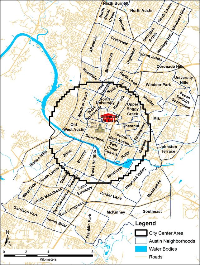
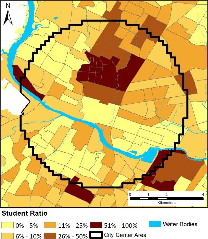
3 We show the spatial distribution of two of our demographic variables in Figure 4. Lower
4 income areas tend to be on the eastern side of the city, with the wealthiest neighborhoods in the
5 northwest. Higher student populations overlap with some of the lower income areas but are
6 generally near the University of Texas campus. These variables are discussed further in our
7 spatial analysis.
8
131 Figure 3 – Neighborhoods in Austin, Texas. Source: City of Austin, Geospatial Services – Data Development.
2
3 Figure 4: Median Annual Income and Student Ratio by Census Block Group in central Austin.
4
5 Table 1: Summary of trip statistics between Aug 16th, 2018 and Feb 28th, 2019.
All Weekdays Weekends Mornings Evenings
& holidays (7AM–10AM) (4PM–7PM)
Trips 2,237,588 1,427,282 810,306 182,005 396,853
Trips % 100% 64% 36% 8% 18%
Avg. trips per day 11,358 10,895 12,277 924 1,877
Median trip distance (meters) 971 917 1,094 869 996
Median trip duration (minutes) 6.6 5.92 8.58 4.98 6.6
6
71
2 Figure 5: Hourly trip distribution on weekdays and on weekends/holidays.
3
151 2 Figure 6: Trip destinations distribution by 200 sq. meter grid cells in Austin, TX, between August 16 th, 2018 3 and February 28th, 2019. Trip destination classes were determined by ArcGIS – the intervals follow a 4 geometric series to highlight extreme cases and show the variation in the city center. 5
1   Methods

 2   Our key research question focuses on understanding the patterns of e-scooter usage. Are these

 3   used for commute trips or recreation? Do they serve various trip types, such as short trips?

 4   Consistent with work on bikesharing, our purpose is to explore whether these issues can be

 5   determined from trip patterns and spatial analysis.

 6           As previously indicated, we examine the central area of the city. We overlay this with

 7   grids and determine the total e-scooter check-outs (departures) and returns (arrivals) in each grid

 8   cell. We have 1342 grid cells of 200x200 meters (0.002°x0.002°), about 40,000 square meters

 9   per cell.

10           A Moran’s I test showed that both departure and arrival values are spatially

11   autocorrelated, hence there is a need for a spatial regression to account for unobserved spatial

12   phenomena that are associated with e-scooter usage. We estimated a Spatial Lag model and

13   Spatial Durbin model. In a Spatial Lag model, , where is a spatial autoregressive coefficient, and

14   W is a spatial weights matrix (Anselin, 2001). In this model, the value of yi depends on the value

15   of yj and vice versa. In a Spatial Durbin model, where and are spatial autoregressive

16   coefficients, and W is a spatial weights matrix. Spatial Durbin models include the spatial effect

17   of the independent variables (Mur and Angulo, 2005). We used a contiguity-based weights

18   matrix which allows bordering cells to influence the outcome variable.

19           Both the Spatial Lag and Spatial Durbin models are linear models and require a normally

20   distributed dependent variable. Our dependent variable, however, is count data, typically

21   estimated with a Poisson or Negative Binomial model. As previously indicated, we focus only on

22   the central part of the city, thus we remove most cells with zero counts. We add one to each

23   dependent variable and take the natural logarithm of the value, thus approximating a normal

                                                     17
1 distribution, allowing us to estimate linear models. We log-transform the independent variables 2 as well for consistency and ease of interpretation. We add one to the values of variables prior to 3 the log transformation, thus avoiding dropping zero values. 4 We also estimate Geographically Weighted Regression (GWR) models. This model 5 performs a series of local linear regressions, and provides a unique regression coefficient for 6 each cell in our grid (Fotheringham, 2009). Each local regression includes the cells within a 7 specified bandwidth. We used the ArcGIS Desktop 10.5.1 GWR tool which computes the 8 optimal fixed bandwidth length based on Akaike Information Criterion. The bandwidth length 9 used was 3430 meters. The GWR model is a more flexible model formulation and provides an 10 interpretation of the variability of coefficient estimates in our study area. We examine how the 11 income coefficient varies across space, providing us with more information on how the income 12 of an area is associated with e-scooter trips. 13 We model both trip departures (i.e., trip generation) in each cell and trip arrivals. The 14 latter provide a closer link between the user’s destination and the associated land use and other 15 spatial features. For trip departures, the user will often need to walk to where an e-scooter is 16 located, leading to less linkage between the spatial factors and the trip starting point, though this 17 would probably be only a minor issue. To obtain a normal distribution we estimated a log-linear 18 model, i.e., the dependent variable is the logarithm of arrivals while the independent variables 19 were not logged. 20
1   Results

 2   We analyzed data for different times of day, as well as for all trips. There are some minor

 3   differences in effect size and significance between the Spatial Lag and the Spatial Durbin

 4   models. We present both; however, the Spatial Durbin model has a slightly higher psuedo-R2 and

 5   we focus on those results. Most estimates are similar among the different times of the day and

 6   the week, except for our weekday morning commute model (i.e., those trips starting between

 7   7am and 10am). We present results for departures (Table 2) and arrivals (Error: Reference source

 8   not found) for all trips and just morning trips for both a Spatial Lag and Spatial Durbin model.

 9          The proportion of residential, commercial, educational, and industrial land uses within a

10   cell have a positive association with both the number of departures and arrivals in that cell.

11   Compared to the reference category (“other land uses,” which includes cemeteries,

12   transportation-related land use, undeveloped land, water, and unclassified land uses), these land

13   uses are associated with more e-scooter trips. The largest coefficients are for commercial and

14   industrial land uses. These results suggest that e-scooters are more likely to be used in these

15   areas, throughout the day. In our Spatial Durbin model, morning departures are associated with

16   residential land uses but not educational land uses. Morning arrivals are associated with

17   educational land uses but not residential.

18          If there is a bike lane or path within the cell there is a positive association with e-scooter

19   departures and arrivals. When a bus stop is within the cell, there is likewise a positive

20   association. These effects are positive for the model predicting all trips and for the model

21   predicting trips during morning hours. Employment density is also positive and statistically

22   significant in all models. The median income in the cell is not statistically significant for almost

23   all the models; we examine the spatial variation of median income using our GWR model in the

                                                      19
1 next section. Intersection density is significant and positive only in the Spatial Durbin models. 2 Our entropy variable, which represents land use mix, is statistically significant and positive for 3 AM trips only. 4 We include the fraction of students living in each area, since the University of Texas is a 5 major part of the city center. Students make up about 9.3% of Austin’s total population, but 6 about 26 to 31% of the population in the central area. The average of our student ratio per cell is 7 16.3%. Associations are positive and significant for both all and morning departures in the 8 Spatial Lag model, for all arrivals in the Spatial Lag model, and for all and morning arrivals in 9 the Spatial Durbin model. This does suggest that students are using e-scooters. 10 We also control for distance from the central point of the city (defined as the intersection 11 of Congress Avenue and 11th Street). Statistically significant effects are found in the Spatial Lag 12 model for all departures and arrivals, with fewer trips as distance to the city center increases. 13 Distance was not significant in the Spatial Durbin models except for the morning arrivals. 14
1    Table 2: Spatial Lag and Spatial Durbin Log-Log regression results for trip origins.

                                                                                                                  Log of morning             Log of morning departures
                                                    Log of all                Log of all departures
                                                                                                                     departures                     (7am – 10am)
Dependent variable:                                departures                   Spatial Durbin
                                                                                                                   (7am – 10am)                    Spatial Durbin
                                                   Spatial Lag
                                                                              β                                     Spatial Lag                 β
Independent:                                Coef.      t-stat       Coef.     t-stat       Coef.    t-stat      Coef.    t-stat       Coef.     t-stat       Coef.    t-stat
(intercept)                                      1.566     2.37**       2.423 2.93***                               1.754 2.66***         2.593 3.09***
Log of percent residential land use (0-1)        0.671 2.94***          1.403 4.64***         -1.393 -2.78***       0.364        1.57     1.001 3.22***         -1.319 -2.56***
Log of percent commercial land use (0-1)         0.715     2.06**       1.891 4.45***         -3.100 -4.01***       0.625      1.78*      1.573 3.60***         -2.835 -3.56***
Log of percent institutional land use (0-1)      0.172         0.56     0.042         0.11     0.622        0.92   -0.136       -0.44    -0.288        -0.72     0.454        0.66
Log of percent educational land use (0-1)        0.510       1.84*      0.655       1.74*     -0.186       -0.30    0.200        0.71     0.138         0.36     0.096        0.15
Log of percent industrial land use (0-1)         1.212     2.26**       1.706 2.72***         -1.286       -1.16    1.004      1.84*      1.521     2.36**      -1.633       -1.43
Log of percent recreation land use (0-1)         0.335         1.40     0.539       1.75*     -0.661       -1.28   -0.132       -0.54     0.190         0.60    -0.871       -1.64
Bikeways in cell (dummy – 0/1)                   0.294 5.24***          0.275 4.61***          0.046        0.39    0.217 3.81***         0.225 3.68***         -0.032       -0.26
Log of median annual income (thousands
of US $)                                        -0.028        -0.79     0.051         0.67    -0.109       -1.04   -0.062     -1.69*      0.015         0.19    -0.110       -1.02
Bus stops in cell (dummy – 0/1)                  0.507 8.51***          0.513 8.53***         -0.250     -1.79*     0.489 8.08***         0.494 7.99***         -0.146       -1.02
Log of employment density
(employments/sq.km)                              0.086 6.22***          0.108 6.48***         -0.016       -0.54    0.085 6.07***         0.088 5.15***          0.027        0.89
Log of intersection density
(intersections/sq.km)                           -0.013        -0.29     0.334 3.66***         -0.464 -3.99***      -0.064       -1.40     0.157       1.67*     -0.334 -2.80***
Log of entropy (0-1)                             0.538         1.63     0.509         1.43     0.993        1.40    0.812    2.42**       0.746     2.04**       0.888        1.21
Log of student ratio (students/total
population)                                      0.432     2.11**       0.832         1.31    -0.611       -0.84    0.813 3.79***         0.993         1.52    -0.360       -0.48
Log of distance to city center (meters)         -0.228 -3.17***        -0.475        -0.82     0.235        0.39   -0.243 -3.33***        0.152         0.26    -0.412       -0.66
rho                                              0.812 44.25***         0.814 39.76***                              0.783 39.16***        0.769   33.11***
Nagelkerke Pseudo R2                            0.7920                 0.8007                                      0.7840                0.7894
  2 Note: reference category for land use is “other”; ‘bikeways’ refers to both on-street bike lanes and off-road bike paths; * p < 0.10, ** p < 0.05, *** p < 0.01.

  3    Table 3: Spatial Lag and Spatial Durbin Log-Log regression results for trip destinations.

Dependent variable:                            Log of all arrivals                Log of all arrivals             Log of morning       Log of morning arrivals (7am – 10am)
                                                 Spatial Lag                       Spatial Durbin                    arrivals                    Spatial Durbin

                                                                                        21
β (7am – 10am) β
Spatial Lag
Independent: Coef. t-stat Coef. t-stat Coef. t-stat Coef. t-stat Coef. t-stat Coef. t-stat
(intercept) 1.501 2.46** 2.326 3.03*** 2.593 3.09*** 2.022 3.22***
Log of percent residential land use (0-1) 0.726 3.45*** 1.421 5.12*** -1.246 -2.71*** 1.001 3.22*** 0.148 0.70 -1.456 -3.07***
Log of percent commercial land use (0-1) 0.698 2.18** 1.735 4.44*** -2.674 -3.77*** 1.573 3.60*** 0.655 2.02** -2.401 -3.29***
Log of percent institutional land use (0-1) 0.229 0.82 0.161 0.45 0.498 0.81 -0.288 -0.72 0.021 0.07 -0.081 -0.13
Log of percent educational land use (0-1) 0.491 1.92* 0.554 1.60 0.065 0.11 0.138 0.36 0.597 2.30** 0.144 0.25
Log of percent industrial land use (0-1) 1.140 2.30** 1.544 2.68*** -0.986 -0.97 1.521 2.36** 0.948 1.89* -1.743 -1.66*
Log of percent recreation land use (0-1) 0.279 1.27 0.345 1.22 -0.339 -0.72 0.190 0.60 -0.231 -1.04 -0.629 -1.29
Bikeways in cell (dummy – 0/1) 0.260 5.03*** 0.232 4.25*** 0.084 0.77 0.225 3.68*** 0.200 3.81*** -0.013 -0.12
Log of median annual income (thousands
of US $) -0.021 -0.64 0.069 1.00 -0.126 -1.32 0.015 0.19 -0.061 -1.79* -0.106 -1.07
Bus stops in cell (dummy – 0/1) 0.417 7.58*** 0.420 7.60*** -0.226 -1.77* 0.494 7.99*** 0.354 6.36*** -0.074 -0.56
Log of employment density
(employments/sq.km) 0.074 5.83*** 0.095 6.20*** -0.012 -0.46 0.088 5.15*** 0.089 6.85*** 0.025 0.90
Log of intersection density
(intersections/sq.km) 0.007 0.17 0.412 4.93*** -0.523 -4.90*** 0.157 1.67* -0.070 -1.69* -0.370 -3.36***
Log of entropy (0-1) 0.455 1.49 0.506 1.55 0.638 0.98 0.746 2.04** 0.591 1.91* 0.494 0.74
Log of student ratio (students/total
population) 0.404 2.14** 0.961 1.65* -0.810 -1.21 0.993 1.52 0.630 3.22*** 0.027 0.04
Log of distance to city center (meters) -0.221 -3.33*** -0.549 -1.03 0.317 0.57 0.152 0.26 -0.254 -3.67*** -0.333 -0.59
rho 0.825 46.82*** 0.828 42.33*** 0.769 33.11*** 0.775 37.90***
Nagelkerke Pseudo R2 0.8014 0.8115 0.7894 0.7985
1 Note: reference category for land use is “other”; ‘bikeways’ refers to both on-street bike lanes and off-road bike paths; * p < 0.10, ** p < 0.05, *** p < 0.01.
221 Geographically Weighted Regression
2 GWR models estimate the effect of local rather than global independent variable
3 coefficients by including only a limited region for estimating the variable coefficients for each
4 study unit. This can provide some greater insight into the determinants of usage as GWR
5 produces both global and local coefficients, the latter varying by grid cell. We estimated models
6 for two dependent variables – all arrival trips and morning arrival trips. Given the different
7 model formulation, coefficient estimates cannot be directly compared with our Spatial Lag and
8 Spatial Durbin models. We examined marginal effects and found similar results to those in our
9 prior models; these are omitted for brevity and we focus on the spatial distribution of the
10 coefficient estimates.
11 Among the 14 independent variables included in the GWR model, we present the results
12 for residential, income, and student ratio in Figure 7. Green shading is for positive coefficient
13 values, while red indicates negative values. Insignificant coefficient values (i.e., p>.05) are
14 omitted. Residential land use has a positive influence on trip arrivals around the south and the
15 west of the city center, but not in the downtown, the University of Texas campus and its
16 surrounding area. This may imply that people who use the service in this area, do not use it to go
17 home or live in a mixed land-use area, or in mixed-use developments (defined in our dataset as
18 commercial land use). In the morning model, however, residential land use is negatively
19 associated with trip arrivals across the city center.
20 Income coefficient patterns are generally similar in both models, although income was
21 significant only in the morning arrivals Spatial Durbin model. The central, northern and western
22 parts of the city center are more affluent, and the eastern part is less affluent. In addition, the
231 median income around the University of Texas is very low, while the student ratio is very high.
2 In both models, the e-scooter usage in the northern and western part of the city center is
3 negatively associated with median income – higher income is associated with fewer trip arrivals
4 and lower income is associated with more trip arrivals. The southeast is an exception with higher
5 income associated with more trip arrivals, but not for morning trips.
6 The coefficient on the fraction of students in the population (student ratio) is relatively
7 similar in both models. The student ratio exceeds 25% around the University of Texas and the
8 northern part of the city center, and also in Pleasant Valley in the eastern part of Riverside. The
9 GWR results show that areas with more students in the northeastern part generate more trips, and
10 areas with fewer students in the western part, where the student ratio is relatively low, generate
11 more trips. The difference between the models suggests that students are probably a major source
12 of usage and imply that many of the morning trips are students.
13 The spatial distribution of other coefficients, not presented in Figure 7, provide some
14 additional insights. In general, land use variables seems to have greater influence in areas where
15 they are scarcer. This is also true for bikeways, population density, and bus stops, but not for
16 other variables. Unlike the Spatial Lag and Spatial Durbin results, distance from the CBD has a
17 stronger effect for all the arrival trips rather than for morning trips. In both GWR models,
18 distance from the CBD seems to be less important for those using the service in the northern part
19 of the city center.
241
2 Figure 7 - GWR results for all and morning arrivals. All the presented values are significant (p < 0.05).
251 Variation in the Coefficients for Income
2 The GWR analysis indicates that the coefficient estimates for median annual income vary
3 throughout the city. Bikesharing services have long struggled to serve low socio-economic
4 populations, and cities have had difficulty engaging populations in low-income areas (Caspi and
5 Noland, 2019). The Spatial Lag results show that income is not a significant predictor for general
6 e-scooter sharing trips. However, the influence of income varies throughout the city center and
7 for weekday morning trips. Our GWR analysis allows us to examine the spatial variation in
8 income coefficients; we then regress those coefficients on the same spatial factors to examine
9 how the income coefficient (or sensitivity of response) varies with those factors.
10 The purpose of this analysis is to determine why there is spatial variation in income
11 coefficients. What are the underlying spatial factors that lead to larger marginal effects in some
12 areas of the city and lower marginal effects (or even negative) in other parts of the city? We are
13 not aware of other studies of shared services examining the source of this variation.
14 In order to understand what is associated with income having a positive or negative effect
15 on e-scooter use, we regressed the income coefficients of both GWR models. We set
16 insignificant coefficients to zero for this analysis. We used a linear regression with the same
17 independent variables used for the Spatial Lag model, including median income. The results are
18 in Table 4.
19 Table 4: Linear regression results for the GWR income coefficients.
Dependent: Income coefficient in Dependent: Income coefficient in
GWR Arrivals - all GWR Arrivals - mornings
Independent: Estimate t-stat Estimate t-stat
(Intercept) -2.63E-03 -2.81*** 2.59E-03 4.25***
Percent residential land use (0-1) -4.06E-03 -5.21*** -3.15E-03 -6.21***
percent commercial land use (0-1) -4.07E-03 -3.16*** -3.99E-03 -4.76***
26Percent institutional land use (0-1) -7.77E-04 -0.67 -1.93E-03 -2.57**
Percent educational land use (0-1) -1.38E-03 -1.34 -1.68E-03 -2.51**
Percent industrial land use (0-1) 8.55E-03 3.82*** 4.19E-03 2.88***
Percent recreation land use (0-1) -5.25E-03 -6.15*** -3.54E-03 -6.38***
Bikeways in cell (dummy – 0/1) 2.00E-04 0.72 -9.64E-05 -0.53
Median annual income (thousands of US $) -3.59E-05 -7.93*** -3.81E-05 -12.93***
Bus stops in cell (dummy – 0/1) -2.63E-04 -0.89 -6.72E-05 -0.35
Employment density (employments/sq.km) -4.74E-10 -0.13 -1.32E-09 -0.54
Intersection density (intersections/sq.km) 3.59E-05 5.82*** 9.90E-06 2.47**
Entropy (0-1) 3.04E-03 2.44** 1.85E-03 2.27**
Student ratio (students/total population) -1.46E-03 -1.94* -3.77E-03 -7.70***
Distance to city center (meters) 6.24E-07 4.01*** -5.79E-07 -5.72***
1 Note: reference category for land use is “other”; bikeways refers to both on-street bike lanes and off-road bike paths;
2 * p < 0.10, ** p < 0.05, *** p < 0.01.
3 All land uses have a negative influence on the income coefficient except industrial land
4 uses, which have a positive influence. In cells with more residential land use, for example, the
5 income coefficient is lower, i.e. lower income is associated with more trips. Income itself also
6 negatively affects the income coefficient – as income in an area rises, the association between
7 income and e-scooter usage becomes more strongly negative. This effect is stronger for all the
8 arrival trips, rather than the morning trips. Entropy positively affects the coefficient; hence, the
9 higher the mix of land uses, the higher the usage in high-income areas. This suggests that high
10 earners in mixed-use neighborhoods are different from high earners in neighborhoods that are
11 more residential in character; the former are more likely to use e-scooters than are the latter, all
12 else equal. We find something similar for students: low-income neighborhoods that are home to
13 a lot of students see more trips than do low-income neighborhoods with fewer students.
14 Discussion and Conclusions
15 Our study examined travel behavior patterns of shared e-scooter use in Austin, Texas. We found
16 that people use e-scooters almost exclusively in central Austin, mainly in and around downtown
271 Austin and the University of Texas, similar to the findings of previous studies (Bai and Jiao,
2 2020; Jiao and Bai, 2020).
3 Descriptive data suggest that commuting is not the main trip purpose for shared e-scooter
4 users in Austin. The hourly weekday trip distribution does not show a two-peak pattern, during
5 morning and evening commuting times, but rather displays a long afternoon plateau. Moreover,
6 the average daily usage is higher on weekends and holidays. This suggests that users mainly use
7 e-scooters for purposes other than commuting, similar to shared e-scooters in other cities
8 (Mathew et al., 2019; McKenzie, 2019; Noland, 2019). Other studies have suggested that most
9 trips are recreational (Bai and Jiao, 2020; Mathew et al., 2019; McKenzie, 2019), however we
10 found that e-scooter usage is less likely to start and end in recreational areas, and more likely to
11 do so in residential, commercial and industrial areas.
12 Usage of e-scooters is associated with areas with high employment rates, and in areas
13 with bicycle infrastructure, compatible with the findings of many bikesharing studies (Buck and
14 Buehler, 2012; Buehler and Dill, 2016; El-Assi et al., 2017; Faghih-Imani et al., 2014; Faghih-
15 Imani and Eluru, 2015; Fishman, 2016; Heinen et al., 2010; Li et al., 2018; Lin et al., 2018;
16 Mateo-Babiano et al., 2016; Sun et al., 2018; Wang et al., 2018, 2016; Zhang et al., 2017). This
17 implies that more bicycle infrastructure may increase scooter usage.
18 Trip origins and destinations are also associated with bus stop locations, suggesting that
19 people may link e-scooter and bus trips. However a deeper investigation of this matter in Austin
20 found that e-scooter users do not link trips with transit (Zuniga-Garcia and Machemehl, 2020).
21 Income does not affect the general usage but does affect morning trips – the lower the income in
22 the area, the more departures and arrivals take place on weekday mornings. Finally, distance to
281 the CBD matters in the morning models; morning trips are more concentrated around the center
2 of Austin’s core.
3 Results from our models suggest that e-scooter trips are taking place around most types
4 of land uses in Austin, TX. Surprisingly, the many government offices in Texas’ capital,
5 represented as “institutional” in our model, did not produce as many e-scooter trips as other
6 places in central Austin.
7 Many e-scooter operators and advocates wish to encourage increased use among lower-
8 income populations. Our findings show that in central Austin, people use shared e-scooters
9 regardless of the affluence of the neighborhood. This does not provide evidence of who is using
10 e-scooters, but does suggest that they are broadly used throughout different neighborhoods. Our
11 GWR modeling results show that in most of the city center usage is higher in less affluent areas.
12 However, these areas are populated with students who likely have lower incomes, but not low
13 socio-economic status. This point is further strengthened in our analysis of the spatial variation
14 of income’s effect on scooter usage; in areas with more students, the association between lower
15 incomes and e-scooter usage is stronger. This suggests that e-scooter sharing services can work
16 well in college towns or on campuses. However, efforts are needed to increase usage in areas
17 with lower incomes.
18 One limitation is that we do not have information on how e-scooter companies deploy
19 and reposition their fleets. This may affect usage in lower income areas if fewer e-scooters are
20 deployed to these neighborhoods. It would not be unsurprising if e-scooter operators deploy
21 their vehicles in neighborhoods with larger student populations but not in low-
22 sociodemographics neighborhoods, although we have no information or evidence regarding this.
291 Our study is limited to assessing the spatial patterns and associations of shared e-scooters
2 in Austin. It does not include information regarding users, their demographics, or their
3 motivations. These can only be implied from our data which is aggregate areal demographic
4 data, land use, and median income. Moreover, we cannot assume that users live in the location of
5 their trip origin or destination. This is clearly an area for more research. Other limitations include
6 the spatial accuracy of trip origins and destinations. GPS devices have an accuracy of about 5
7 meters but are not free of errors. While we cleaned our dataset, errors in location data may
8 remain.
9 Shared e-scooters are a new mode of transportation and if successful can provide an
10 environmentally friendly mode that serves many needs. Our study sheds light on how they are
11 being used in one city, Austin, Texas. Patterns of usage may differ depending on the
12 demographics, road networks, transit availability, and spatial patterns of different cities. Non-
13 commuting e-scooter utilitarian trips appear high in Austin. However, whether shared e-scooters
14 can reduce car usage and benefit the environment is yet to be determined.
15
16
17 AUTHOR CONTRIBUTION STATEMENT
18 The authors confirm contribution to the paper as follows: study conception and design: all; data
19 collection: all; analysis and interpretation of results: all; draft manuscript preparation: all. All
20 authors reviewed the results and approved the final version of the manuscript.
301 References
2 Ahillen, M., Mateo-Babiano, D., Corcoran, J., 2016. Dynamics of bike sharing in Washington,
3 DC and Brisbane, Australia: Implications for policy and planning. International Journal
4 of Sustainable Transportation 10, 441–454.
5 https://doi.org/10.1080/15568318.2014.966933
6 Allem, J.-P., Majmundar, A., 2019. Are electric scooters promoted on social media with safety in
7 mind? A case study on Bird’s Instagram. Preventive Medicine Reports 13, 62–63.
8 https://doi.org/10.1016/j.pmedr.2018.11.013
9 Anselin, L., 2001. Spatial Econometrics, in: Palgrave Handbook of Econometrics: Volume 1,
10 Econometric Theory. Kluwer, pp. 310–330.
11 Badeau, A., Carman, C., Newman, M., Steenblik, J., Carlson, M., Madsen, T., 2019. Emergency
12 department visits for electric scooter-related injuries after introduction of an urban rental
13 program. The American Journal of Emergency Medicine.
14 https://doi.org/10.1016/j.ajem.2019.05.003
15 Bai, S., Jiao, J., 2020. Dockless E-scooter usage patterns and urban built Environments: A
16 comparison study of Austin, TX, and Minneapolis, MN. Travel Behaviour and Society
17 20, 264–272. https://doi.org/10.1016/j.tbs.2020.04.005
18 Beecham, R., Wood, J., 2014. Exploring gendered cycling behaviours within a large-scale
19 behavioural data-set. Transportation Planning and Technology 37, 83–97.
20 https://doi.org/10.1080/03081060.2013.844903
21 Bernatchez, A.C., Gauvin, L., Fuller, D., Dubé, A.S., Drouin, L., 2015. Knowing about a public
22 bicycle share program in Montreal, Canada: Are diffusion of innovation and proximity
23 enough for equitable awareness? Journal of Transport & Health 2, 360–368.
24 https://doi.org/10.1016/j.jth.2015.04.005
25 Bresler, A.Y., Hanba, C., Svider, P., Carron, M.A., Hsueh, W.D., Paskhover, B., 2019.
26 Craniofacial injuries related to motorized scooter use: A rising epidemic. American
27 Journal of Otolaryngology. https://doi.org/10.1016/j.amjoto.2019.05.023
28 Buck, D., Buehler, R., 2012. Bike Lanes and Other Determinants of Capital Bikeshare Trips.
29 Presented at the TRB 2012 Annual Meeting, p. 11.
30 Buck, D., Buehler, R., Happ, P., Rawls, B., Chung, P., Borecki, N., 2013. Are bikeshare users
31 different from regular cyclists? A first look at short-term users, annual members, and area
32 cyclists in the Washington, DC, region. Transportation Research Record: Journal of the
33 Transportation Research Board 112–119.
34 Buehler, R., Dill, J., 2016. Bikeway Networks: A Review of Effects on Cycling. Transport
35 Reviews 36, 9–27. https://doi.org/10.1080/01441647.2015.1069908
36 Caspi, O., Noland, R.B., 2019. Bikesharing in Philadelphia: Do lower-income areas generate
37 trips? Travel Behaviour and Society 16, 143–152.
38 https://doi.org/10.1016/j.tbs.2019.05.004
39 Census Bureau, 2017. TIGER/Line® Shapefiles [WWW Document]. URL
40 https://www.census.gov/cgi-bin/geo/shapefiles/index.php?
41 year=2015&layergroup=Urban+Areas (accessed 11.1.18).
42 City of Austin Texas, 2020. Dockless Vehicle Trips [WWW Document]. URL
43 https://data.austintexas.gov/Transportation-and-Mobility/Dockless-Vehicle-Trips/7d8e-
44 dm7r (accessed 6.19.19).
311 City of Austin Texas, 2019a. Land Use Inventory Detailed [WWW Document]. Austin. URL
2 https://data.austintexas.gov/Locations-and-Maps/Land-Use-Inventory-Detailed/fj9m-
3 h5qy (accessed 7.11.19).
4 City of Austin Texas, 2019b. Street Centerlines [WWW Document]. Austin. URL
5 https://data.austintexas.gov/Locations-and-Maps/Street-Centerline/m5w3-uea6 (accessed
6 7.11.19).
7 City of Austin Texas, 2019c. CapMetro Shapefiles - JUNE 2018 [WWW Document]. URL
8 https://data.texas.gov/Transportation/CapMetro-Shapefiles-JUNE-2018/rwce-6ann
9 (accessed 7.11.19).
10 El-Assi, W., Salah Mahmoud, M., Nurul Habib, K., 2017. Effects of built environment and
11 weather on bike sharing demand: a station level analysis of commercial bike sharing in
12 Toronto. Transportation 44, 589–613. https://doi.org/10.1007/s11116-015-9669-z
13 Faghih-Imani, A., Eluru, N., 2015. Analysing bicycle-sharing system user destination choice
14 preferences: Chicago’s Divvy system. Journal of Transport Geography 44, 53–64.
15 https://doi.org/10.1016/j.jtrangeo.2015.03.005
16 Faghih-Imani, A., Eluru, N., El-Geneidy, A.M., Rabbat, M., Haq, U., 2014. How land-use and
17 urban form impact bicycle flows: evidence from the bicycle-sharing system (BIXI) in
18 Montreal. Journal of Transport Geography 41, 306–314.
19 https://doi.org/10.1016/j.jtrangeo.2014.01.013
20 Ferster, C., Fischer, J., Manaugh, K., Nelson, T., Winters, M., 2019. Using OpenStreetMap to
21 inventory bicycle infrastructure: A comparison with open data from cities. International
22 Journal of Sustainable Transportation. https://doi.org/10.1080/15568318.2018.1519746
23 Fishman, E., 2016. Bikeshare: A review of recent literature. Transport Reviews 36, 92–113.
24 Fishman, E., Washington, S., Haworth, N., 2013. Bike share: a synthesis of the literature.
25 Transport reviews 33, 148–165.
26 Fishman, E., Washington, S., Haworth, N., Mazzei, A., 2014. Barriers to bikesharing: an analysis
27 from Melbourne and Brisbane. Journal of Transport Geography 41, 325–337.
28 Fotheringham, A.S., 2009. Geographically Weighted Regression, in: The SAGE Handbook of
29 Spatial Analysis. SAGE Publications.
30 Gebhart, K., Noland, R.B., 2014. The impact of weather conditions on bikeshare trips in
31 Washington, DC. Transportation 41, 1205–1225. https://doi.org/10.1007/s11116-014-
32 9540-7
33 Goodman, A., Cheshire, J., 2014. Inequalities in the London bicycle sharing system revisited:
34 impacts of extending the scheme to poorer areas but then doubling prices. Journal of
35 Transport Geography 41, 272–279. https://doi.org/10.1016/j.jtrangeo.2014.04.004
36 Hall, M., 2017. Bird scooters flying around town. Santa Monica Daily Press.
37 Heinen, E., Wee, B. van, Maat, K., 2010. Commuting by Bicycle: An Overview of the Literature.
38 Transport Reviews 30, 59–96. https://doi.org/10.1080/01441640903187001
39 Hochmair, H.H., Zielstra, D., Neis, P., 2013. Assessing the Completeness of Bicycle Trail and
40 Designated Lane Features in OpenStreetMap for the United States and Europe. Presented
41 at the Transportation Research Board 92nd Annual MeetingTransportation Research
42 Board.
43 Hollingsworth, J., Copeland, B., Johnson, J.X., 2019. Are e-scooters polluters? The
44 environmental impacts of shared dockless electric scooters. Environ. Res. Lett. 14,
45 084031. https://doi.org/10.1088/1748-9326/ab2da8
321 Jiao, J., Bai, S., 2020. Understanding the Shared E-scooter Travels in Austin, TX. ISPRS
2 International Journal of Geo-Information 9, 135. https://doi.org/10.3390/ijgi9020135
3 Kim, K., 2018. Investigation on the effects of weather and calendar events on bike-sharing
4 according to the trip patterns of bike rentals of stations. Journal of Transport Geography
5 66, 309–320. https://doi.org/10.1016/j.jtrangeo.2018.01.001
6 LDA Consulting, 2012. Capital bikeshare 2011 member survey report. LDA Consulting,
7 Washington, D.C.
8 Li, H., Ding, H., Ren, G., Xu, C., 2018. Effects of the London Cycle Superhighways on the
9 usage of the London Cycle Hire. Transportation Research Part A: Policy and Practice
10 111, 304–315. https://doi.org/10.1016/j.tra.2018.03.020
11 Lin, J.-J., Zhao, P., Takada, K., Li, S., Yai, T., Chen, C.-H., 2018. Built environment and public
12 bike usage for metro access: A comparison of neighborhoods in Beijing, Taipei, and
13 Tokyo. Transportation Research Part D: Transport and Environment 63, 209–221.
14 https://doi.org/10.1016/j.trd.2018.05.007
15 Mateo-Babiano, I., Bean, R., Corcoran, J., Pojani, D., 2016. How does our natural and built
16 environment affect the use of bicycle sharing? Transportation Research Part A: Policy
17 and Practice 94, 295–307. https://doi.org/10.1016/j.tra.2016.09.015
18 Mathew, J.K., Liu, M., Seeder, S., Li, H., Bullock, D.M., 2019. Analysis of E-Scooter Trips and
19 Their Temporal Usage Patterns. Institute of Transportation Engineers. ITE Journal;
20 Washington 89, 44–49.
21 Mayhew, L.J., Bergin, C., 2019. Impact of e-scooter injuries on Emergency Department imaging.
22 Journal of Medical Imaging and Radiation Oncology 0. https://doi.org/10.1111/1754-
23 9485.12889
24 McKenzie, G., 2019. Spatiotemporal comparative analysis of scooter-share and bike-share usage
25 patterns in Washington, D.C. Journal of Transport Geography 78, 19–28.
26 https://doi.org/10.1016/j.jtrangeo.2019.05.007
27 McKenzie, G., 2018. Docked vs. Dockless Bike-sharing: Contrasting Spatiotemporal Patterns
28 (Short Paper), in: Wagner, M. (Ed.), . Presented at the 10th International Conference on
29 Geographic Information Science (GIScience 2018), Melbourne, Australia.
30 https://doi.org/10.4230/lipics.giscience.2018.46
31 Micromobility | AustinTexas.gov - The Official Website of the City of Austin [WWW
32 Document], n.d. URL http://austintexas.gov/micromobility (accessed 6.19.19).
33 Mur, J., Angulo, A., 2005. A closer look at the Spatial Durbin Model. Presented at the European
34 Regional Science Association 45th Congress, European Regional Science Association,
35 Amsterdam.
36 Murphy, E., Usher, J., 2015. The Role of Bicycle-sharing in the City: Analysis of the Irish
37 Experience. International Journal of Sustainable Transportation 9, 116–125.
38 https://doi.org/10.1080/15568318.2012.748855
39 NACTO, 2019. Shared Micromobility in the U.S.: 2018. National Organization of City
40 Transportation Officials.
41 Noland, R.B., 2019. Trip patterns and revenue of shared e-scooters in Louisville, Kentucky.
42 Transport Findings 7747. https://doi.org/10.32866/7747
43 Noland, R.B., Smart, M.J., Guo, Z., 2016. Bikeshare trip generation in New York City.
44 Transportation Research Part A: Policy and Practice 94, 164–181.
45 https://doi.org/10.1016/j.tra.2016.08.030
33You can also read