Identifying synergies in private and public transportation
←
→
Page content transcription
If your browser does not render page correctly, please read the page content below
Identifying synergies in private and public transportation
                                                Iva Bojic1,∗ , Dániel Kondor1 , Wei Tu (涂伟)2 , Ke Mai (麦可)2 , Paolo Santi3,4 , Carlo Ratti3
                                                                        1
                                                                       Singapore-MIT Alliance for Research and Technology, Singapore
                                                           2
                                                               Guangdong Key Laboratory of Urban Informatics, Department of Urban Informatics,
                                                                   School of Architecture and Urban Planning, Shenzhen University, China
                                                                          3
                                                                             Senseable City Laboratory, MIT, Cambridge MA, USA
                                                                         4
                                                                            Istituto di Informatica e Telematica del CNR, Pisa, Italy
                                                                                          ∗
                                                                                            E-mail: ivabojic@mit.edu
arXiv:2009.09659v1 [cs.CY] 21 Sep 2020

                                                                                                   November 21, 2021

                                         Abstract
                                         In this paper, we explore existing synergies between pri-                                      transit (bus / train)
                                         vate and public transportation as provided by taxi and bus
                                         services on the level of individual trips. While these modes

                                                                                                                          travel time
                                         are typically separated for economic reasons, in a future
                                         with shared Autonomous Vehicles (AVs) providing cheap                                                                       ridesharing
                                         and efficient transportation services, such distinctions will                                                                   car / taxi
                                         blur. Consequently, optimization based on real-time data
                                         will allow exploiting parallels in demand in a dynamic way,
                                         such as the proposed approach of the current work. New
                                         operational and pricing strategies will then evolve, provid-
                                                                                                                                                 energy use / cost
                                         ing service in a more efficient way and utilizing a dynamic
                                         landscape of urban transportation. In the current work,
                                         we evaluate existing parallels between individual bus and                    Figure 1: Illustration of tradeoffs in travel time, cost and
                                         taxi trips in two Asian cities and show how exploiting these                 energy use that is typical in today’s transportation. Car
                                         synergies could lead to an increase in transportation service                and bus icons by Rediffusion and Rainbow Designs from
                                         quality.                                                                     the Noun Project, used under CC BY.

                                         1     Introduction                                                           tion modes often have much lower total travel times at the
                                                                                                                      cost of significantly higher fleet size and total energy use,
                                         In today’s transportation industry, there is a large oper-                   as shown in Fig. 1.
                                         ational gap between private end-to-end services such as                         Such tradeoffs are important, as transportation today is
                                         taxis1 and ride-hailing, and fixed-route public transporta-                  a part of every good or service produced [3], while com-
                                         tion such as buses and subways [1, 2]. While the former                      muting takes up an important portion of people’s time [4].
                                         provide more convenience for passengers and usually a sig-                   This way, the choices for transportation have overarching
                                         nificantly shorter travel time at a higher price, the latter                 effects for economic productivity and quality of life [5]. In
                                         operate on inflexible schedules and routes, with many in-                    many developed countries, government policies in the past
                                         termediate stops that slow down the service, but at a sig-                   decades have favored private transportation by ensuring
                                         nificantly lower cost to passengers, operators and society.                  low fuel prices and investing in road infrastructure, despite
                                         Looking from a global perspective, we can contrast the to-                   the increasing evidence of the significant societal cost of
                                         tal passenger travel time with the total fleet size and vehi-                private transportation, up to 28 times higher than public
                                         cle distance traveled. Public transportation modes have a                    transportation [6]. Due to the large increase of vehicles
                                         higher travel time, but achieve this with a lower fleet size,                on roads, cities around the world face significant problems
                                         total travel distance and energy use. Private transporta-                    due to congestion; in peak hours, public transportation
                                                                                                                      options can provide a shorter travel time when separated
                                            1 We note that the taxi market is often highly regulated and in
                                                                                                                      from general traffic [7]. A high usage of private vehicles
                                         some cases, taxi companies are government-owned. Due to these
                                         reasons, some authors consider taxis as part of public transportation.
                                                                                                                      also contributes to local emissions, while globally, the high
                                         Nevertheless, for the purposes of the current work, we believe the           total energy use of the transportation sector is also con-
                                         important distinction is along the lines presented here.                     cerning [8].

                                                                                                                  1
The traffic situation is even more problematic in devel- the potential benefits for the passengers who would reg-
oping countries where underinvestment in both private and ularly take bus services if paired with the taxi passen-
public transportation infrastructure resulted in significant gers who take the same route at approximately the same
congestion and delays for users of both modes. With the time. With this pairing, the bus passengers can reduce
lack of public transportation alternatives, the majority of their travel time and the taxi passengers can save money,
commuters often use private modes, such as in the Klang while the volume of traffic would not increase. There are
Valley, Malaysia, where only 17% of daily trips are made two main research questions in this paper: (i) what is the
using public transport [9], compared to more than 60% or percentage of bus passengers who could be matched with
90% of trips made in Singapore and Hong Kong, respec- the taxi passengers if we assume that both taxi and bus
tively [10]. demand is based on today’s situation; and (ii) what is the
With the expected availability of Autonomous Vehicles average travel time saved per a bus trip for the passengers
(AVs) in near future [11, 12, 13], it will be possible for who were matched. Answering these questions can give
the above situation to change, with in-between solutions us an understanding about the potential of partial integra-
becoming viable [14, 15]. Eliminating drivers’ salary can tion of public and private transportation systems. Namely,
result in Autonomous Mobility On Demand (AMOD) ser- while not significantly affecting existing taxi passengers or
vices becoming dramatically cheaper than services with hu- increasing road traffic, our analysis shows a way to im-
man drivers today [16, 17]. This raises concerns if public prove public transportation experience by reducing a travel
transportation can remain competitive [18]. At the same time and increasing a travel comfort for its passengers. By
time, these cost savings will allow public transportation showing case studies in two different cities (Singapore and
operators to explore innovative solutions with new vehicle Shenzhen), our analysis also hints at the generalizability of
form factors to provide increased level of service for com- our findings, at least in the context of Asian metropolises.
muters without increasing costs. The rest of the paper is organized as follows. Section 2
Some of these effects can already be seen with the dis- gives an overview of the datasets used in our analysis. As
ruptive changes caused by the emergence of Transporta- we are comparing bus and taxi trips for two different cities,
tion Network Companies (TNCs), such as Uber, DiDi or we have four different sources describing people’s mobility
Grab [19]. While originally perceived as competitors to patterns. Section 3 describes our methodology, formally
taxis [20, 21], it soon became apparent that TNCs serve defining the matching process between trips and explain-
as competitors to public transportation as well [22, 23, 24]. ing the steps of our analysis in detail. Section 4 shows
Nevertheless, it has been observed that TNCs can also serve our main findings answering the two research questions we
a complementary role, especially in areas and time periods pose in this paper, i.e. the percentage of bus trips that can
that are not served well by current public transportation be matched and the average travel time saved for those
options [25, 26]. matched trips. Finally, Section 5 discusses our results and
In addition to TNCs disrupting transportation sys- shows directions for future work.
tems today, Mobility-as-a-Service (MaaS) [27] also brings
changes in public transportation by aiming to explicitly 2 Data
integrate public and private transportation modes. The
effects of MaaS on public transportation were explored in In this paper, we compare the percentage of bus trips that
different countries such as Sweden [28], Finland [29] and can be shared with taxi trips in two cities, namely Singa-
Germany [30]. Focus of those research studies was mostly pore and Shenzhen. The taxi dataset for Singapore con-
on how to find a “sweet spot” that supports innovation, sists of more than 30 million of taxi trips recorded for 77
but also secures public benefits. Further research has ex- consecutive days, a total of 10 weeks. Distribution of the
plored such an integration and collaboration specifically in number of taxi trips per each day is given in SI Fig. S1,
the context of shared AVs and AMOD services [31, 32]. where each day in a week is marked with a different color.
In this work, we aim to characterize potential benefits What we can observe from the figure is that the number of
of a more flexible cooperation between private and public taxi trips is always the largest on Friday and the smallest
transportation services by investigating existing synergies on Sunday, while between Sunday and Friday the number
between public and private transportation. Potential ap- gradually grows. What is also evident is that there is a
plications can depend on the pricing and market strategy of little of variance across the observed weeks, with an ex-
operators and policy decisions of governments to maximize ception of the second to last week, where Thursday was a
public good. We envision a future where private (i.e. non- public holiday and consequently the number of taxi trips
shared) on-demand transportation remains a “premium” on the preceding Wednesday was higher and on Thursday
option, while a flexible array of shared options provide bet- itself it was significantly lower. From those 10 weeks, we
ter convenience, shorter travel times in a more efficient way chose the second week as a representative week for further
than current public transportation and ridesharing services analysis. In Shenzhen, we used one week of taxi trips as
can. In this context, our goal is to inform about the share- well, that has 3 million trips in total, while in Singapore,
ability potential that can be most easily realized thanks to we have about 2.8 million trips in the chosen week. Neither
the reduced cost of AV operations. dataset includes any personal data of passengers.
More specifically, in this paper, we investigate what are Bus trips for Shenzhen were collected during the same
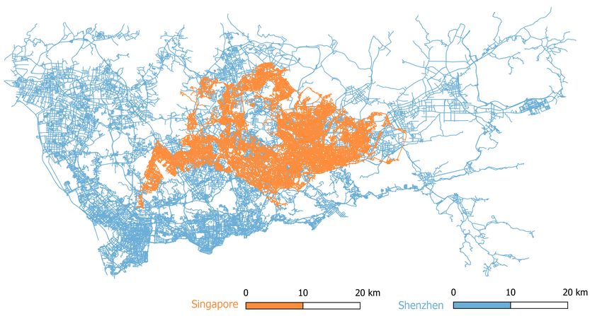
2Figure 2: The road networks for Singapore and Shenzhen displayed on the same scale.
week as taxi trips and include tap-in data for 15 million the clustering procedure, the road network for Singapore
trips in total, made by 6.5 million anonymized passen- had more than 50,000 nodes and 120,000 edges, while the
gers who are represented by randomly generated IDs used one for Shenzhen had almost 40,000 nodes and 100,000
throughout the data collection period. Using the algo- edges.
rithm developed by Tu et al. [33], we were able to infer When comparing the numbers of records in Singapore
destinations for a total of 3.4 million trips that we use and Shenzhen datasets, what we can conclude is that
in the following analysis (for a more detailed description, the number of taxi trips for both cities is comparable,
see the Supplementary Material). Bus trips for Singapore i.e. around 3 million, with Singapore recording a bit less.
were generated based on the aggregate counts of bus usage However, due to limitation of Shenzhen bus dataset not
available in the DataMall public interface [34]. The data including tap-out data, out of around 15 million records
is based on smart card tap-in and tap-out events, and in- initially recorded in the dataset, we were able to use only a
cludes the hourly total number of bus trips made between bit more than 25%. With that being said, what we can see
any two bus stops in the city over the course of a month, is a large difference in the ratio of bus trips recorded in each
separately counted for weekdays and weekends. In total, city, with Singapore having around six times more bus trips
we have generated a bit more than 20 million bus trips than Shenzhen. However, on the other hand, in Shenzhen
for one week. We generated daily numbers based on this, dataset we have individual trips with the exact starting
assuming a Poisson distribution of individual daily counts time, which is information that is missing from Singapore
and assigned trips in the hourly intervals based on a Pois- dataset as there we only have aggregated numbers of peo-
son distribution of bus arrivals as described in more detail ple traveling between each pair of origin/destination bus
in the Supplementary Material. stops within one hour. When comparing the numbers of
nodes in each city’s road network, we note that the area of
In addition to the taxi and bus datasets, we also down-
Shenzhen is 2.8 larger than Singapore; this indicates that
loaded the road networks for the two cities from Open-
the road network of Shenzhen is more sparse, which is also
StreetMap [35]. For Singapore, we used a bounding box
evident in Fig. 2.
that covers the whole island, and then manually excluded
roads that provide connections to Malaysia, and finally,
kept the largest connected component of the resulting road 3 Methodology
network, yielding the network shown in Fig. 2. For Shen-
zhen, we used a bounding box that covers the official The taxi trip datasets for both Singapore and Shenzhen
boundary of Shenzhen and then removed the connections are in the same format of Global Positioning System (GPS)
to Hong Kong and kept the largest connected component, traces. As taxis move through the city, their geolocation
similarly to the case of Singapore. We further processed (i.e. latitude and longitude) is recorded at irregular time
the raw networks by performing a friend-of-friend cluster- intervals. In that sense, for each taxi trip in the dataset,
ing, grouping together nodes with a threshold radius of there are multiple spatio-temporal points allowing us to
20 m, reducing the network size to simplify processing and reconstruct the route that it took. As the first step, we
remove uncertainties from small errors in GPS data. After mapped the taxi trajectories to the road network, using
3the algorithm of Yang et al. [36]. The result of this proce- pair to be exactly the same as a taxi trip O/D pair in order
dure is an ordered list of network nodes that are present in for two trips to be matched, but simply that a subset of
the most likely trajectory corresponding to the trip. The the taxi trip matches the bus trip O/D pair.
advantage of this method is that we are not limited by The selection of the time buffer tB assumes that a pas-
the irregularity in recording GPS points, and we can thus senger would go to the bus stop tB time before boarding
identify all possible matching opportunities. A taxi trip Ti the bus and is willing to wait up to tB after the original
is then represented as an ordered set of tuples (nij , tij ), departure time if matched with a taxi trip that still arrives
j = 1, 2 . . . Ni , where nij denotes the sequence of road earlier at their destination. Of course, in a more detailed
network nodes identified as part of the trajectory, tij are model, tB could be selected on a per-trip basis, if an esti-
the estimated timestamps for each node based on the GPS mate of the actual waiting time for the bus and individual
timestamps and finally Ni denotes the total number road tolerance for extra waiting time could be established. The
network nodes in a trajectory Ti . travel time saving τij is defined as the actual travel time
For each bus trip, we assign a set of road network nodes saving, i.e. how much faster the trip is realized with the
as candidate sets for the beginning and end of the trip, taxi than the original bus trip. Notably, we do not include
based on their proximity to the coordinates of the bus stop. any time savings due to the taxi trip starting earlier. This
This way, a bus trip Bi is represented as the following: likely underestimates the total time savings achievable to
Bi = {Si , ti,s , Ei , ti,e }, where Si and Ei are the candidate passengers, but since we do not have a reliable estimate of
sets for the start and end of the trip respectively, and ti,s waiting times for bus passengers, we chose to only focus on
and ti,e are the estimated start and end times of the trip. the part of the trip spent traveling. We acknowledge that
We control the selection of the candidate sets with the pa- minimizing waiting time could be an important additional
rameter d that we refer to as the spatial buffer. For the goal of any combined on-demand mobility service.
special value of d = 0, the candidate sets only include the Pairs in Mf represent all possible sharing opportunities
closest node to the bus stop. For d > 0, the candidate and form a bipartite graph, where the τij time savings are
sets include all road network nodes within an Euclidean interpreted as edge weights. Potentially, any trip will have
distance of d. In practice, we use d = 0, 100 m and 200 m. multiple match candidates (i.e. will be present with a de-
The significance of d is to allow a match where the pick-up gree > 1). Using this graph, we then calculate a maximal
does not exactly take place at the bus stop. Since the actual weighted matching [37, 38] to arrive at an ideal assignment
start of a passenger’s trip is typically not the exact location of trips that maximize time saved for bus passengers while
of a bus stop, this buffer is interpreted in the sense that respecting the condition that each trip can be matched only
instead of going to the bus stop, a passenger would walk at most once. To be able to provide a tractable solution
to a pick-up location that is within an acceptable distance and also to limit inconvenience to taxi passengers, we do
of their original location. not consider the possibility of a taxi trip being matched to
We then compile a set of potential matches between bus multiple bus trips consecutively; if there are multiple such
and taxi trips, M f, as pairs of trips where a taxi trip includes candidates, we choose the one that contributes to maximiz-
road network nodes from the start and the end candidate ing time savings globally.
set of a bus trip in the correct order. We also require that
the node in the bus start set is visited by the taxi within
a short time interval, tB , defined as a time buffer within 4 Results
the start of the bus trip and that the end node is visited
The results of our analysis are presented with two main
earlier than the end of the bus trip, allowing time savings
figures, each one answering one main research question.
for the bus passenger. Formally, we define:
Namely, Fig. 3 shows the percentage of bus passengers who
were able to be matched with taxi passengers, while Fig. 4
f = {(Ti , Bj , τij )} ∀(i, j), where ∃ k, l
M
shows the average travel time saved per a matched bus
(1) 1 ≤ k < l ≤ Ni trip expressed in minutes. Results for the percentage of
(2) nik ∈ Sj and nil ∈ Ej matched trips and average time savings are calculated in
such that (3) |tik − tj,s | < tB (1) one hour windows in the time period of significant bus ser-
(4) tj,e − til > 0 vice, between i.e. 6 AM and 11 PM in both cities; corre-
(5) τij ≡ (tj,e − tj,s ) − (til − tik ) > 0 spondingly, x-axes are limited between 6 AM and 10 PM.
y-axes show the percentage of matched trips in Fig. 3 and
The conditions listed here guarantee that (1) road net- the time savings in minutes in Fig. 4. Each main figure
work nodes are visited in the correct order; (2) both the is divided into eight sub-figures denoting results for Singa-
start and the end of the bus trip are visited by the taxi pore and Shenzhen separately, as well as for different time
trip; (3) the bus passenger can take the taxi within a tB buffers and for two days (Wednesday and Saturday) that
temporal buffer of the start of their original trip; (4) they represent typical results for workdays and weekends. Each
arrive earlier than with their original bus trip; and (5) that panel shows results for three different values of the space
the actual travel time is shorter, where we define τij as the buffer, i.e. d = 0, 100 m and 200 m. Results for the re-
travel time saving achieved. Note that this matching pro- maining days of week are displayed in the Supplementary
cedure does not require a bus trip origin/destination (O/D) Material as Figs. S6 – S9.
4Wednesday, 1 minute buffer Wednesday, 5 minute buffer
Singapore Shenzhen Singapore Shenzhen
35
Percentage of bus trips matched 30
Search radius
25
200 m
20
100 m
15
0m
10
5
0
6 8 10 12 14 16 18 20 22 6 8 10 12 14 16 18 20 22 6 8 10 12 14 16 18 20 22 6 8 10 12 14 16 18 20 22
hour hour
Saturday, 1 minute buffer Saturday, 5 minute buffer
Singapore Shenzhen Singapore Shenzhen
35
Percentage of bus trips matched
30
Search radius
25
200 m
20
100 m
15
0m
10
5
0
6 8 10 12 14 16 18 20 22 6 8 10 12 14 16 18 20 22 6 8 10 12 14 16 18 20 22 6 8 10 12 14 16 18 20 22
hour hour
Figure 3: Ratio of bus trips that could be served as a shared trip with a taxi passenger. Results are displayed for
Shenzhen and Singapore respectively in the left and right panels. The top row shows results Wednesday and the bottom
row shows results for Saturday. Results for the rest of the week are presented in the Supplementary Material, in Figs. S6
and S8. Figures on the left correspond to a time buffer of 1 minute and figures on the right correspond to a time buffer
of 5 minutes.
As expected, the percentage of bus trips matched goes night hours. The reason for that kind of behavior is that
up as we increase the space and time buffers. For exam- there is a little of difference in bus distribution in Shen-
ple, if we set the time buffer to 1 minute, the percentage zhen between Wednesday and Saturday, while the number
of matched bus trips on Wednesday for Singapore for the of taxi trips on Saturday is on average larger than the one
radius of 200 meters is on average a bit less than 10% in on Wednesday. The same patterns are observed for 5 min-
morning hours (i.e. between 9 to 12 AM), drops to 5% utes time buffers, but as expected with a higher percentage
around 6 PM and then goes up to a bit more than 10% in of bus trips matched. However, the percentage of bus trips
the late night (i.e. around 10 PM). Similar, but slightly matched go much higher for Shenzhen than for Singapore,
lower percentages of matched trips could be also observed around 15% on Wednesday and 20% on Saturday for 200
for Shenzhen. However, there is a bit of different pattern meters search radius.
during the day with two drops around 10 AM and midday When looking at the average absolute travel time saved
and a much sharper drop around 6 PM. The reason for for Singapore and Shenzhen (as illustrated in Fig. 4), what
this is the drop of the total number of taxi trips during we can see is that the bus passengers in Singapore who get
those periods as shown in SI Fig. S3 in the Supplemen- matched with the taxi riders can save a bit more than 4
tary Material. Namely, whereas the total number of taxi minutes per their trip for 1 minute time buffer and 200 m
trips in Singapore stays more stable from 10 AM to 1 PM, space buffer. At the same time, the time savings in Shen-
in Shenzhen there are two drops at 10 AM and midday. zhen (with the same parameters) on average are a bit less
Given that the number of bus trips during the same time than 4 minutes. The time savings with 5 minutes time
does not change that much either, chances for the bus pas- radius and 200 m space buffer can go over 5 minutes in
sengers to share a ride with the taxi passengers are lower the case of Singapore and over 4 minutes in the case of
around 10 AM and 12 PM. Shenzhen. This also indicates that the increased sharing
For Saturday, the percentage of matched bus tips for opportunities contribute to more travel time savings even
Singapore is slightly lower than 10% and is flatter dur- without including the effect of potentially starting trips ear-
ing the day, with no drop around 6 PM and also rising in lier that is possible with a larger tB time buffer. Regarding
late night hours. In Shenzhen, the percentage of bus trips time patterns, in Singapore we can see larger time savings
matched on Saturday is slightly larger than 10%, with two around 6 AM and 6 PM for both Wednesday and Satur-
drops around 1 PM and 6 PM and a large spike in late day, while the pattern for Shenzhen is flatter and also does
5Wednesday, 1 minute buffer Wednesday, 5 minute buffer
Singapore Shenzhen Singapore Shenzhen
8
Avg. time saved per matched trip [min] 7
Search radius
6
5 200 m
4 100 m
3
0m
2
1
0
6 8 10 12 14 16 18 20 22 6 8 10 12 14 16 18 20 22 6 8 10 12 14 16 18 20 22 6 8 10 12 14 16 18 20 22
hour hour
Saturday, 1 minute buffer Saturday, 5 minute buffer
Singapore Shenzhen Singapore Shenzhen
8
Avg. time saved per matched trip [min]
7
Search radius
6
5 200 m
4 100 m
3
0m
2
1
0
6 8 10 12 14 16 18 20 22 6 8 10 12 14 16 18 20 22 6 8 10 12 14 16 18 20 22 6 8 10 12 14 16 18 20 22
hour hour
Figure 4: Average time saved by bus passengers who are able to be served in a shared trip. Results are displayed for
Shenzhen and Singapore respectively in the left and right panels. The top row shows results Wednesday and the bottom
row shows results for Saturday. Results for the rest of the week are presented in the Supplementary Material, in Figs. S7
and S9. Figures on the left correspond to a time buffer of 1 minute and figures on the right correspond to a time buffer
of 5 minutes.
not show a lot of variety between a workday and weekend. will contribute to vehicles being utilized more, e.g. by in-
This is an interesting finding as when comparing the aver- troducing services based on shared rides in medium-sized
age bus trip lengths of Singapore and Shenzhen (as shown vehicles (6-10 passengers) [15], which would provide travel
in SI Fig. S5), we can see that on average, bus trips in time benefits over public buses and reduced fleet size com-
Singapore are shorter (i.e. mean for Singapore is around pared to taxi and ride-hailing services.
10 minutes and for Shenzhen 14 minutes). This is under- In this paper, we thus analyzed the first step of integrat-
standable given that the area of Shenzhen is significantly ing public and private transportation using today’s travel
larger. Consequently, when putting time savings into a per- demand. Using mobility patterns recorded by taxi com-
spective, this means that on average, absolute travel time panies and bus operators in Singapore and Shenzhen, we
saved in Singapore is up to 50% of mean bus duration and investigated how passengers on public transportation can
around 30% for Shenzhen. reduce their travel time if paired with already existing taxi
riders. In our proposed framework, we can identify three
stakeholders - passengers taking public transportation, taxi
5 Discussion riders, and the local government being responsible for pub-
lic roads. The matching concept explored in our work
Until very recently, private and public transportation have presents a Pareto improvement from the current situation,
been two systems that were very much separated [1, 6]. i.e. some stakeholders’ experience benefits, while none of
However, with the emergence of Transportation Network them experience losses: the travel time is reduced for some
Companies (TNCs) and Mobility-as-a-Service (MaaS) con- public transportation passengers, the costs are reduced for
cepts, those lines are becoming more unclear [19, 22, 25, some taxi passengers, while the total number of cars and
28]. This will be even more evident once Shared Au- traffic on the road does not increase.
tonomous Vehicles (SAVs) hit the roads bringing further The results of our analysis showed that between 10 to
disruptive changes to urban mobility [11, 12, 13, 18]. If 20 percent of bus riders could be potentially matched with
drivers’ costs are removed from the equation, vehicles of taxi riders, which would contribute to on average between
different, more flexible capacities would be able to oper- 4 to 6 minutes of savings of their travel time. These results
ate in public transportation services as well. In practice, are consistent across two cities in Asia, although there are
this will allow transportation services to be more fluid and individual differences in the temporal pattern of match-
6ing ratios. The main source of difference is explained by References
how the total volume of taxi and bus trips changes during
the day. Namely, first we see a clear difference between [1] C. Jacques, K. Manaugh, A. M. El-Geneidy, Rescuing the
the distribution of total bus trips in Singapore between a captive [mode] user: An alternative approach to transport
market segmentation, Transportation 40 (3) (2013) 625–
weekday and a weekend, whereas this difference is less ob-
645. doi:10.1007/s11116-012-9437-2.
vious in case of Shenzhen. This possibly means that in
Shenzhen, more people also work on Saturdays. Second, [2] V. Verbavatz, M. Barthelemy, Critical factors for mitigat-
the total amount of taxi trips on Saturday in Shenzhen is ing car traffic in cities, PLOS ONE 14 (7) (2019) e0219559.
larger than on Wednesday, which is not true for Singapore. doi:10.1371/journal.pone.0219559.
In conclusion, our analysis shows that there is a practi- [3] D. L. Greene, D. W. Jones, The full costs and benefits
cal potential for partial integration of public and private of transportation: Contributions to theory, method and
transportation even under the current conditions. This is measurement; with 62 tables, Springer Science & Business
an important first step when envisioning a future where Media, 1997.
AV technology allows a variety of novel transportation ser- [4] C. Ingraham, The astonishing human potential wasted on
vice types. Future work might look into extensions where commutes, Washington Post 25.
bus passengers are not only matched with taxis in an op-
[5] A. Lowrey, Your commute is killing you, New York, NY:
portunistic manner, but with alternative service providers
Slate.
that can operate with medium sized (i.e. 6-10 passenger)
vehicles with the specific goal of providing a faster, more [6] A. Jakob, J. L. Craig, G. Fisher, Transport cost analysis: a
convenient and demand-responsive transportation alterna- case study of the total costs of private and public transport
tive to buses. We note that previous work in this area was in Auckland, Environmental Science & Policy 9 (1) (2006)
limited to using taxi trips as an estimate of demand [15]; 55–66. doi:10.1016/j.envsci.2005.09.001.
our results show the importance of including the complete [7] L. A. Lindau, D. Hidalgo, D. Facchini, Curitiba, the cradle
picture of urban transportation demand, i.e. both public of bus rapid transit, Built Environment 36 (3) (2010) 274–
and private transportation users. Furthermore, while our 282. doi:10.2148/benv.36.3.274.
work shows a potential for matching trips, any such ser-
[8] S. Jia, H. Peng, S. Liu, X. Zhang, Review of trans-
vice will face challenges in implementing user interaction
portation and energy consumption related research, Jour-
solutions that can be conveniently used without exclud- nal of Transportation Systems Engineering and Infor-
ing groups of users, e.g. those who do not use a smart- mation Technology 9 (3) (2009) 6–16. doi:10.1016/
phone. This means that investigating new user interaction S1570-6672(08)60061-6.
concepts for the fluid transportation services of tomorrow
will become increasingly important as more and more op- [9] O. Chiu Chuen, M. R. Karim, S. Yusoff, Mode choice
between private and public transport in Klang Val-
timization opportunities in on-demand transportation are
ley, Malaysia, The Scientific World Journal 2014 (2014)
realized.
394587. doi:10.1155/2014/394587.
[10] J. Luk, P. Olszewski, Integrated public transport in singa-
pore and hong kong, Road & Transport Research 12 (4)
(2003) 41–51. https://search.proquest.com/docview/
Acknowledgments 215248165
[11] D. J. Fagnant, K. Kockelman, Preparing a nation for
This research is supported by the Singapore Ministry of autonomous vehicles: Opportunities, barriers and policy
National Development and the National Research Founda- recommendations, Transportation Research Part A: Pol-
tion, Prime Minister’s Office, under the Singapore-MIT Al- icy and Practice 77 (2015) 167–181. doi:10.1016/j.tra.
liance for Research and Technology (SMART) programme. 2015.04.003.
We also thank RATP, Dover Corporation, Allianz, Teck
[12] OECD International Transport Forum, Urban Mo-
Resources, Lab Campus, Anas S.p.A., Ford, ENEL Foun-
bility System Upgrade: How shared self-driving
dation, the Amsterdam Institute for Advanced Metropoli-
cars could change city traffic, Tech. rep. (2015).
tan Solutions, the cities of Laval, Curitiba, Stockholm and http://www.internationaltransportforum.org/Pub/
Amsterdam, and all of the members of the MIT Senseable pdf/15CPB_Self-drivingcars.pdf
City Laboratory Consortium for supporting this research.
Wei Tu acknowlegdes the funding of Nature Science Foun- [13] D. Stead, B. Vaddadi, Automated vehicles and how they
dation of China (No.4207010598). may affect urban form: A review of recent scenario studies,
Cities 92 (September 2018) (2019) 125–133. doi:10.1016/
j.cities.2019.03.020.
[14] D. Christie, A. Koymans, T. Chanard, J. M. Lasgouttes,
V. Kaufmann, Pioneering Driverless Electric Vehicles in
Declarations of interests Europe: The City Automated Transport System (CATS),
Transportation Research Procedia 13 (2016) 30–39. doi:
The authors declare no competing interest. 10.1016/j.trpro.2016.05.004.
7[15] J. Alonso-Mora, S. Samaranayake, A. Wallar, E. Fraz- [28] G. Smith, J. Sochor, I. M. Karlsson, Mobility as a ser-
zoli, D. Rus, On-demand high-capacity ride-sharing via vice: Development scenarios and implications for pub-
dynamic trip-vehicle assignment, Proceedings of the lic transport, Research in Transportation Economics 69
National Academy of Sciences 114 (3) (2017) 462–467. (2018) 592–599. doi:10.1016/j.retrec.2018.04.001.
arXiv:\protect\vrulewidth0pt\protect\href{http:
//arxiv.org/abs/1507.06011}{arXiv:1507.06011}, [29] S. Heikkilä, Mobility as a service-a proposal for action
doi:10.1073/pnas.1611675114. for the public administration, case helsinki, Master’s the-
sis, Aalto University (2014). https://aaltodoc.aalto.
[16] L. D. Burns, W. C. Jordan, B. A. Scarborough, fi/handle/123456789/13133
Transforming Personal Mobility, Tech. rep., The
Earth Institute, Columbia University (2013). http:// [30] J. Schikofsky, T. Dannewald, M. Kowald, Exploring mo-
wordpress.ei.columbia.edu/mobility/files/2012/12/ tivational mechanisms behind the intention to adopt mo-
Transforming-Personal-Mobility-Aug-10-2012.pdf bility as a service (MaaS): Insights from Germany, Trans-
portation Research Part A: Policy and Practice 131 (2020)
[17] C. Brownell, A. Kornhauser, A Driverless Alternative Fleet 296–312. doi:10.1016/j.tra.2019.09.022.
Size and Cost Requirements for a Statewide Autonomous
Taxi Network in New Jersey, Transportation Research [31] M. Salazar, F. Rossi, M. Schiffer, C. H. Onder, M. Pavone,
Record 2416 (2014) 73–81. doi:10.3141/2416-09. On the Interaction between Autonomous Mobility-on-
Demand and Public Transportation Systems, in: 21st In-
[18] B. W. Smith, Managing Autonomous Transportation De- ternational Conference on Intelligent Transportation Sys-
mand, Santa Clara Law Review 52 (4) (2012) 1401–1422. tems (ITSC), 2018, pp. 2262–2269. arXiv:1804.11278,
doi:10.1525/sp.2007.54.1.23. doi:10.1109/ITSC.2018.8569381.
[19] S. Shaheen, N. Chan, Mobility and the sharing economy: [32] Y. Shen, H. Zhang, J. Zhao, Integrating shared au-
Potential to facilitate the first-and last-mile public tran- tonomous vehicle in public transportation system: A
sit connections, Built Environment 42 (4) (2016) 573–588. supply-side simulation of the first-mile service in Singa-
doi:10.2148/benv.42.4.573. pore, Transportation Research Part A: Policy and Practice
[20] D. N. Anderson, “Not just a taxi”? For-profit ridesharing, 113 (April) (2018) 125–136. doi:10.1016/j.tra.2018.
driver strategies, and VMT, Transportation 41 (5) (2014) 04.004.
1099–1117. doi:10.1007/s11116-014-9531-8. [33] W. Tu, R. Cao, Y. Yue, B. Zhou, Q. Li, Q. Li, Spatial vari-
[21] M. Glöss, M. McGregor, B. Brown, Designing for labour: ations in urban public ridership derived from GPS trajecto-
Uber and the on-demand mobile workforce, in: Proceed- ries and smart card data, Journal of Transport Geography
ings of the 2016 CHI conference on human factors in 69 (2018) 45–57. doi:10.1016/j.jtrangeo.2018.04.013.
computing systems, 2016, pp. 1632–1643. doi:10.1145/
[34] DataMall, (web interface), https://www.
2858036.2858476.
mytransport.sg/content/mytransport/home/dataMall/
[22] S. Feigon, C. Murphy, Shared mobility and the transfor- dynamic-data.html, accessed 2019-11-01. Bus data for
mation of public transit, no. Project J-11, Task 21, Trans- January 2019 was downloaded on 2019-02-13. (2019).
portation Research Board, 2016. doi:10.17226/23578.
[35] M. Haklay, P. Weber, Openstreetmap: User-generated
[23] L. Rayle, D. Dai, N. Chan, R. Cervero, S. Shaheen, Just street maps, IEEE Pervasive Computing 7 (4) (2008) 12–
a better taxi? A survey-based comparison of taxis, tran- 18. doi:10.1109/MPRV.2008.80.
sit, and ridesourcing services in San Francisco, Transport
Policy 45 (2016) 168–178. doi:10.1016/j.tranpol.2015. [36] C. Yang, G. Gidófalvi, Fast map matching, an algorithm
10.004. integrating hidden markov model with precomputation, In-
ternational Journal of Geographical Information Science
[24] Y. E. Hawas, M. N. Hassan, A. Abulibdeh, A multi-criteria 32 (3) (2018) 547–570. arXiv:https://doi.org/10.1080/
approach of assessing public transport accessibility at a 13658816.2017.1400548, doi:10.1080/13658816.2017.
strategic level, Journal of Transport Geography 57 (2016) 1400548.
19–34.
[37] J. Edmonds, Paths, trees, and flowers, Canadian Jour-
[25] S. T. Jin, H. Kong, D. Z. Sui, Uber, public transit, and nal of Mathematics 17 (1965) 449–467. doi:10.4153/
urban transportation equity: A case study in New York CJM-1965-045-4.
City, The Professional Geographer 71 (2) (2019) 315–330.
doi:10.1080/00330124.2018.1531038. [38] B. Dezso, A. Jüttner, P. Kovács, LEMON - An open
source C++ graph template library, Electronic Notes in
[26] R. Grahn, S. Qian, H. S. Matthews, C. Hendrick- Theoretical Computer Science 264 (5) (2011) 23–45. doi:
son, Are travelers substituting between transportation 10.1016/j.entcs.2011.06.003.
network companies (TNC) and public buses? A
case study in Pittsburgh, Transportationdoi:10.1007/ [39] C. Zhong, E. Manley, S. M. Arisona, M. Batty, G. Schmitt,
s11116-020-10081-4. Measuring variability of mobility patterns from multi-
day smart-card data, Journal of Computational Science
[27] S. Hietanen, S. Sahala, Mobility as a service. Forum 9 (2015) 125–130. doi:10.1016/j.jocs.2015.04.021.
Virium Helsinki (2014). https://www.itscanada.ca/
files/MaaS%20Canada%20by%20Sampo%20Hietanen%
20and%20Sami%20Sahala.pdf
8Supplementary Material
Supplementary Figures Figure S1 shows the number of taxi trips in Singapore for each of 77 consecutive days
recorded in our dataset. Figure S3 shows distribution of the number of taxi and bus trips per hour on Wednesday in
Singapore and Shenzhen, while Figure S4 presents the same distributions, but for Saturday. Figure S5 shows distribution
of bus trip duration per hour on Wednesday and Saturday in Singapore and Shenzhen. Figures S6 and S8 show the
percentage of shareable trips for the rest of the weekdays that were not included in Fig. 3 in the main text (i.e. Monday,
Tuesday, Thursday, Friday and Sunday). Figures S7 and S9 show the average time savings for bus passengers on these
days.
Bus trip processing for Shenzhen For Shenzhen, we fused bus GPS trajectories and Smart Card Data (SCD) to
infer bus trips destinations. We inferred the alighting location and time by considering the spatial-temporal regularity
of the SCD user. Firstly, the boarding location of a smart card user was inferred. The continuous bus GPS trajectory
was recovered from GPS records by map matching considering the road network and the delay at the road crossing
[33]. Each bus SCD record was linked to the corresponding trajectory based on the bus identification number. The
recorded time was then used to interpolate the boarding location from the GPS trajectory. Following the direction of
the bus route, we adjusted the boarding location to the nearest bus stop in the bus route. Then, the alighting location
of the SCD record was inferred. The SCD user with a pair with the highly frequent boarding locations were filtered
[39]. Considering the regularity of commuters, the following highly frequently boarding location was recognized as the
alighting location of the preceding SCD record. The alighting time was interpolated according to the corresponding
continuous GPS trajectory.
Bus trip generation for Singapore The bus dataset includes hourly counts of trips between any two bus stops in
Singapore over the course of one month, aggregated separately for weekdays and weekends. As a first step, we calculated
the average hourly counts for each day, by dividing the total numbers with the number of weekdays and weekend days
(including public holidays), i.e. 22 and 9 respectively. Next, we generated realizations of the actual number of bus trips
between each bus stop pair by sampling from a Poisson distribution with the mean given by the average counts. We
repeated this process for each bus stop pair and for each hour of the day when buses are operating. We then distributed
trip start times in the one-hour intervals based on a process where a given number of individually distributed bus
departures were assumed for each bus stop in each hour. To achieve this, we counted the total hourly passenger counts
for each bus stop, denoting by Nij the number of passengers boarding a bus at the ith stop of the jth hour. We then
assumed that the expected number of bus departures in a stop was related to the number of passenger boarding in the
following way:
Nij if Nij < N ∗
α
Bij = (2)
B ∗ + (Nij − N ∗ )/b0 if Nij ≥ N ∗
Note that we defined the relation in Eq. 2 based on our previous work with the bus travel data. In Eq. 2, we used
B ∗ ≡ (N ∗ )α and the numerical parameters were α = 0.7, N ∗ = 200 and b0 = 40. We displayed the relationship between
Bij and Nij in Fig. S2. Using this relationship, we assigned Bij as the expected number of bus departures for every
bus stop and hour and then generated an actual number of departures from a Poisson distribution with Bij mean and
excluding the case when this random choice would give a zero value. As the last step, we distributed departure times
within the one-hour interval among the bus departures using an exponential distribution and normalizing the total
elapsed time and assigned each passenger randomly among the buses, using the departure time of the selected bus as
the trip start time.
9400
Total number of taxi trips (thousands)
300
200
100
0
Sa i
Su t
Mn
Tun
Tun
We
Th d
u
Sa i
Su t
Mn
Tun
We
ed
u
Sa i
Su t
Mn
Tun
We
ed
u
Sa i
Su t
Mn
Tun
We
ed
u
Sa i
Su t
Mn
We
ed
u
Sa i
Su t
Mn
Tun
We
ed
u
Sa i
Su t
Mn
Tun
We
ed
u
Sa i
Su t
Mn
Tun
We
Th d
u
Sa i
Su t
Mn
Tun
We
ed
u
Sa i
Su t
Mn
Tun
We
ed
u
Sa i
Su t
Mn
Tun
We
ed
u
Fr
Fr
Fr
Fr
Fr
Fr
Fr
Fr
Fr
Fr
Fr
o
e
o
Th
o
Th
o
Th
o
Th
o
Th
o
Th
o
e
o
Th
o
Th
o
Th
Days
Figure S1: The number of taxi trips in Singapore per day.
60
Number of hourly bus departures
50
40
30
20
10
0
0 100 200 300 400 500 600 700 800 900 1000
Number of hourly passenger boardings
Figure S2: Empirically motivated relationship between the hourly number of bus passengers in a stop and the expected
number of bus departures, i.e. the relationship described in Eq. 2.
Total number of taxi trips on Wednesday Total number of bus trips on Wednesday
35 350
Singapore Singapore
30 300
Shenzhen Shenzhen
Number of trips (thousands)
Number of trips (thousands)
25 250
20 200
15 150
10 100
5 50
0 0
6 7 8 9 10 11 12 13 14 15 16 17 18 19 20 21 22 6 7 8 9 10 11 12 13 14 15 16 17 18 19 20 21 22
Hour Hour
Figure S3: Comparing the total number of taxi and bus trips on Wednesday in two cities.
10Total number of taxi trips on Saturday Total number of bus trips on Saturday
35 350
Singapore Singapore
30 300
Shenzhen Shenzhen
Number of trips (thousands)
Number of trips (thousands)
25 250
20 200
15 150
10 100
5 50
0 0
6 7 8 9 10 11 12 13 14 15 16 17 18 19 20 21 22 6 7 8 9 10 11 12 13 14 15 16 17 18 19 20 21 22
Hour Hour
Figure S4: Comparing the total number of taxi and bus trips on Saturday in two cities.
Wednesday Saturday
10 10
9 Singapore 9 Singapore
8 Shenzhen 8 Shenzhen
7 7
Frequency [%]
Frequency [%]
6 6
5 5
4 4
3 3
2 2
1 1
0 0
0 5 10 15 20 25 30 35 40 45 50 55 60 0 5 10 15 20 25 30 35 40 45 50 55 60
Duration of bus trip [min] Duration of bus trip [min]
Figure S5: Comparing duration of bus trips on Wednesday and Saturday in two cities. Dashed lines display the mean of
the distributions, which are 9.98 min and 10.03 min in the case of Singapore for Wednesday and Saturday respectively,
and 13.67 min and 14.32 min in the case of Shenzhen.
11Monday, 1 minute buffer Monday, 5 minute buffer
Singapore Shenzhen Singapore Shenzhen
35
Percentage of bus trips matched
30
Search radius
25
200 m
20
100 m
15
0m
10
5
0
6 8 10 12 14 16 18 20 22 6 8 10 12 14 16 18 20 22 6 8 10 12 14 16 18 20 22 6 8 10 12 14 16 18 20 22
hour hour
Tuesday, 1 minute buffer Tuesday, 5 minute buffer
Singapore Shenzhen Singapore Shenzhen
35
Percentage of bus trips matched
30
Search radius
25
200 m
20
100 m
15
0m
10
5
0
6 8 10 12 14 16 18 20 22 6 8 10 12 14 16 18 20 22 6 8 10 12 14 16 18 20 22 6 8 10 12 14 16 18 20 22
hour hour
Thursday, 1 minute buffer Thursday, 5 minute buffer
Singapore Shenzhen Singapore Shenzhen
35
Percentage of bus trips matched
30
Search radius
25
200 m
20
100 m
15
0m
10
5
0
6 8 10 12 14 16 18 20 22 6 8 10 12 14 16 18 20 22 6 8 10 12 14 16 18 20 22 6 8 10 12 14 16 18 20 22
hour hour
Friday, 1 minute buffer Friday, 5 minute buffer
Singapore Shenzhen Singapore Shenzhen
35
Percentage of bus trips matched
30
Search radius
25
200 m
20
100 m
15
0m
10
5
0
6 8 10 12 14 16 18 20 22 6 8 10 12 14 16 18 20 22 6 8 10 12 14 16 18 20 22 6 8 10 12 14 16 18 20 22
hour hour
Figure S6: Percentage of bus trips shareable for weekdays.
12Monday, 1 minute buffer Monday, 5 minute buffer
Singapore Shenzhen Singapore Shenzhen
8
Avg. time saved per matched trip [min]
7
Search radius
6
5 200 m
4 100 m
3
0m
2
1
0
6 8 10 12 14 16 18 20 22 6 8 10 12 14 16 18 20 22 6 8 10 12 14 16 18 20 22 6 8 10 12 14 16 18 20 22
hour hour
Tuesday, 1 minute buffer Tuesday, 5 minute buffer
Singapore Shenzhen Singapore Shenzhen
8
Avg. time saved per matched trip [min]
7
Search radius
6
5 200 m
4 100 m
3
0m
2
1
0
6 8 10 12 14 16 18 20 22 6 8 10 12 14 16 18 20 22 6 8 10 12 14 16 18 20 22 6 8 10 12 14 16 18 20 22
hour hour
Thursday, 1 minute buffer Thursday, 5 minute buffer
Singapore Shenzhen Singapore Shenzhen
8
Avg. time saved per matched trip [min]
7
Search radius
6
5 200 m
4 100 m
3
0m
2
1
0
6 8 10 12 14 16 18 20 22 6 8 10 12 14 16 18 20 22 6 8 10 12 14 16 18 20 22 6 8 10 12 14 16 18 20 22
hour hour
Sunday, 1 minute buffer Sunday, 5 minute buffer
Singapore Shenzhen Singapore Shenzhen
8
Avg. time saved per matched trip [min]
7
Search radius
6
5 200 m
4 100 m
3
0m
2
1
0
6 8 10 12 14 16 18 20 22 6 8 10 12 14 16 18 20 22 6 8 10 12 14 16 18 20 22 6 8 10 12 14 16 18 20 22
hour hour
Figure S7: Average time saved for shareable trips on weekdays.
13Sunday, 1 minute buffer Sunday, 5 minute buffer
Singapore Shenzhen Singapore Shenzhen
35
Percentage of bus trips matched
30
Search radius
25
200 m
20
100 m
15
0m
10
5
0
6 8 10 12 14 16 18 20 22 6 8 10 12 14 16 18 20 22 6 8 10 12 14 16 18 20 22 6 8 10 12 14 16 18 20 22
hour hour
Figure S8: Percentage of bus trips shareable for Sunday.
Friday, 1 minute buffer Friday, 5 minute buffer
Singapore Shenzhen Singapore Shenzhen
8
Avg. time saved per matched trip [min]
7
Search radius
6
5 200 m
4 100 m
3
0m
2
1
0
6 8 10 12 14 16 18 20 22 6 8 10 12 14 16 18 20 22 6 8 10 12 14 16 18 20 22 6 8 10 12 14 16 18 20 22
hour hour
Figure S9: Average time saved for shareable trips on Sunday.
14You can also read