Mapping Spatio-Temporal Soil Erosion Patterns in the Candelaro River Basin, Italy, Using the G2 Model With Sentinel2 Imagery - MDPI

Article

Mapping Spatio-Temporal Soil Erosion Patterns in
the Candelaro River Basin, Italy, Using the G2 Model
With Sentinel2 Imagery
Christos Karydas 1,*, Ouiza Bouarour 2 and Pandi Zdruli 2,*
 1 Remote Sensing Engineer, Mesimeri, Post Office Box 413, 57500 Epanomi, Greece
 2 Soil Science and Natural Resources, International Centre for Advanced Mediterranean
 Agronomic Studies (CIHEAM), Mediterranean Agronomic Institute of Bari,
 Department of Land and Water Resource Management, Via Ceglie 9, 70010 Valenzano, Bari, Italy;
 ouiza.bouarour@gmail.com
 * Correspondence: xkarydas@gmail.com (C.K.); pandi@iamb.it (P.Z.)

 Received: 14 December 2019; 24 February 2020; Published: 27 February 2020

 Abstract: This study aims at mapping soil erosion caused by water in the Candelaro river basin,
 Apulia region, Italy, using the G2 erosion model. The G2 model can provide erosion maps and
 statistical figures at month-time intervals, by applying non data-demanding alternatives for the
 estimation of all the erosion factors. In the current research, G2 is taking a step further with the
 introduction of Sentinel2 satellite images for mapping vegetation retention factor on a fine scale;
 Sentinel2 is a ready-to-use, image product of high quality, freely available by the European Space
 Agency. Although only three recent cloud-free Sentinel2 images covering Candelaro were found in
 the archive, new solutions were elaborated to overcome time-gaps. The study in Candelaro resulted
 in a mean annual erosion rate of 0.87 t ha–1 y–1, while the autumn months were indicated to be the
 most erosive ones, with average erosion rates reaching a maximum of 0.12 t ha–1 in September. The
 mixed agricultural-natural patterns revealed to be the riskiest surfaces for most months of the year,
 while arable land was the most extensive erosive land cover category. The erosion maps will allow
 competent authorities to support relevant mitigation measures. Furthermore, the study in
 Candelaro can play the role of a pilot study for the whole Apulia region, where erosion studies are
 rather limited.

 Keywords: erosion; G2 model; sentinel2

1. Introduction

1.1. Objectives
 In this study, the spatial erosion patterns in the Candelaro river basin, Apulia region (or Puglia
region), in the south of Italy, were mapped on month-time intervals. Candelaro was selected due to
its morphology, land cover, and crop diversity, as well as for being one of the few sloping areas in
Apulia.
 The G2 erosion model was employed as an appropriate tool for high-resolution erosion
assessments, while Sentinel2 satellite imagery was used to detect vegetation patterns in detail
throughout the year. Specific objectives of this study were:
 • To indicate the specific contribution of different land covers to soil erosion in Candelaro,
 especially regarding the seasonal changes of rain intensity and vegetation cover;

Geosciences 2020, 10, 89; doi:10.3390/geosciences10030089 www.mdpi.com/journal/geosciences

Geosciences 2020, 10, 89 2 of 22

 • To introduce Sentinel2 imagery in the vegetation factor algorithm of the G2 methodology,
 thus revising the model; this could be novelty of the current work;
 • To assess the potential of the herewith-revised G2 model, through its application in
 Candelaro, in terms of a pilot study, towards expanding its application at a later time in the
 whole Apulia Region (where erosion studies are rather limited).

1.2. Erosion in Italy
 The Mediterranean region is particularly prone to erosion [1,2], because it is subject to long dry
periods followed by heavy bursts of erosive rain, falling on steep slopes with fragile soils. Erosion
rates are expected to rise during the twenty-first century due to climate change. This will be reflected
by a more dynamic hydrologic cycle that in turn will be associated with frequent torrential rainfall
patterns; thus, increasing water erosion intensity [3]. In addition to that, the impacts by the erosion
process in the Mediterranean regions are the worst compared with other regions in Europe [4–7]. This
is particularly relevant when dealing with typical heavy rainfall events that often characterize the
Mediterranean region and Italy in particular [8].
 Severe soil erosion affects 17% of the land area of Italy; based on OECD data (2008) [9], about
30% of the Italian territory is affected by soil erosion, with rates greater than 10 t ha–1 y–1. The semi-
arid zones of the south of Italy and the islands of Sicily and Sardinia are particularly prone to erosion
due to a combination of climatic factors and rugged terrains, often bare of vegetation because of
historical overgrazing and frequent forest fires [10,11]. Landslides on the other side are estimated to
affect almost half of the Italian cities [12].
 The topic of land degradation due to soil loss by water erosion has been extensively studied in
Italy. Several soil erosion studies [13–17] and numerous publications [11,18–22] focus on different soil
erosion processes. As in many other countries, erosion estimates have also been subject of continuous
debates and adjustments. For instance, the estimates made by Van der Knijff et al. (1999) [14], were
challenged by Grimm et al. (2003) [23] that estimated lower erosion risk rates for the Alps and the
Apennines, and on the contrary, higher ones for the central part of Sicily than those provided by [14].
 According to Costantini and Lorenzetti (2013) [24], critical areas at risk of soil erosion are located
in central and southern Italy, on slopes where agricultural lands are intensively cultivated. The
natural erosion process is typical for several areas of Calabria and Basilicata with the presence of the
so-called calanchi (Figure 1). In contrast, woodlands with the highest risk of erosion and landslides
are more widespread in northern Italy, on the steep slopes of the Alps, and the Apennines. Italy’s
annual average erosion rates are equal or more than 11 t ha–1 y–1 and the annual economic damage
from landslides, floods, and soil erosion is estimated at 900 million euros [24].

 Figure 1. Evidence of natural erosion in sedimentary claystone/siltstone/sandstone formations in
 Calabria, Italy (Photo credit: P. Zdruli).

Geosciences 2020, 10, 89 3 of 22

1.3. The G2 Model
 G2 is an empirical model for soil erosion on month-time intervals, with two distinct modules:
one for soil loss and one for sediment yield [25,26]. The module for soil loss (denoted by G2los) uses
the main empirical formulas of the Universal Soil Loss Equation (USLE) [27,28], which according to
Ferro (2010) [29], is a robust empirical model with a logical structure regarding the variables used to
simulate the physical erosion process.
 With G2los, five input erosion factors are combined in a multiplicative equation, to estimate a
quantitative soil loss output from sheet and interill erosion processes [26]:
 
 = ∙ ∙ (1)
 
 Where Em: soil loss for month m (t ha−1); Rm: rainfall erosivity of month m (MJ mm ha−1 h−1); Vm:
vegetation retention for month m (dimensionless; inversely analogous to C-factor of USLE); S: soil
erodibility (t ha h MJ−1 ha−1 mm−1); T: terrain influence (dimensionless; analogous to LS-factor of
USLE); L: landscape effect (dimensionless; inversely analogous to P-factor of USLE). Compared to
other USLE-family models, an added value of G2 can be considered the possibility for non-
demanding data alternatives for all erosion factors. (Details on the erosion factors are provided in the
Methodology section).
 Developed in 2010, within the framework of GMES Initiative (now, Copernicus Land
Monitoring Service, CLMS) and specifically by the ‘geoland2’ project team [30], the G2 model was
developed with a steady view to serve as an effective decision-making tool based on harmonized
datasets and procedures. Since then, it has been revised through a series of published case studies
conducted in Greece, Bulgaria, Albania, Cyprus [31], and more recently, in Poland [32]. Today, the
G2 model is listed among other well-known models in the ‘Water Erosion Theme’ of the European
Soil Data Centre (ESDAC) of the Joint Research Centre (JRC) [33].
 Up until now, the G2los module relied on the use of the fraction cover (or FCover) layers for the
estimation of the vegetation retention factor, together with information on land cover derived from
CORINE Land Cover (CLC) datasets. Provided by CLMS, FCover layers are available at either 333 m
or 1 km, processed from MERIS or SPOT/VGT images, respectively, on 10-day intervals. FCover
belongs to a set of layers of biophysical properties (known as ‘BIOPAR’ products), provided regularly
by CLMS [34].
 Lately, Sentinel2 imagery provided free by the European Space Agency (ESA), through the
Copernicus Open Access Hub, as a high-resolution dataset on 5-day intervals, offers the possibility
to replace the pre-existing low spatial resolution FCover layers by a higher resolution vegetation
layer. Sentinel2 images are captured by the MultiSpectral Instrument (MSI) and carry 13 spectral
bands ranging from the visible and near-infrared to the short-wave infrared, ready-to-use in an
atmospherically corrected reflectance mode. The spatial resolution varies from 10 to 60 m, depending
on the spectral band, with a 290 kilometers field of view [35,36].

2. Study Area and Dataset

2.1. Study Area
 The Candelaro river basin is in Foggia regional unit, in the northern part of the Apulia Region,
Italy (Figure 2). It comprises a geo-morphological environment typical of the ‘Tavoliere delle Puglie’,
which is the largest alluvial plain in southern Italy and the second largest in Italy [37]. The Candelaro
river basin discharges into the Manfredonia Gulf. The drainage catchment area is 2331 km2, and the
main river course has a length of 67 km. Major streams from north to south, are Macchione Canal and
of the Triolo, Casanova, Salsola, Vulgano, and Celone streams. The mean elevation is 300 m above
sea level, ranging from 0 to 1142 m. A big part of the upland area of the catchment belongs to the
Gargano National Park, founded in 1991. The soils exhibit a texture varying from sandy-clay-loam to
clay-loam or clay. Erosion signs can be observed mainly in the hilly cultivated slopes (Figure 3).

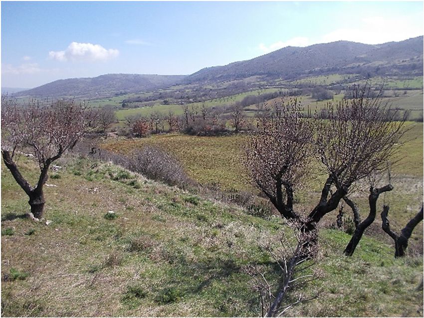
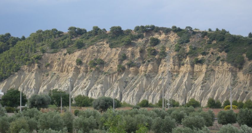
Geosciences 2020, 10, 89 4 of 22

 Figure 2. The Candelaro river basin; location map (left hand side) and anaglyph with the main stream
 course (right hand side).

 (a) (b)

 Figure 3. Typical landscape of Candelaro watershed with agricultural crops in the bottom valleys (a)
 and natural lands on the surrounding slopes (b) (Photo credit: P. Zdruli).

 From 1990 to 2016, the average annual precipitation in the catchment was 570 mm. The
orographic aspects affect rainfall amounts, as well as the patterns of rainfall events. The rainfall is
mostly concentrated in autumn and winter seasons, it is unevenly distributed and often occurs with
high intensity in short duration. The stream flow regime changes rapidly and follows the
precipitation regime closely. The discharge per unit area ranges between 2.6 and 5.6 L s−1 km−2.
 The range of average daily temperature is 12–15 °C. The average annual potential
evapotranspiration is about 1060 mm [38].
 The main economic activity in the plain area is intensive agriculture, the main farm products
being durum wheat, tomatoes, sugar beet, olives, and vineyards. In the mountainous part of the
basin, natural and manmade forest lands and pasture are frequent, occasionally associated with fruit
trees, vineyards, and olive groves [39].

Geosciences 2020, 10, 89 5 of 22

2.2. Dataset Description
 According to the parameters of the G2 erosion factor equations, the following required data
became available to this research (Table 1):
 a. Monthly rainfall figures and number of rainy days per month for the period 2000–2013 from
 13 weather stations throughout the study area (Source: Hydrographic and Mareographic
 Office of Bari for the Basins with the mouth of the Adriatic and Ionian coasts from Candelaro
 to the Lato of Puglia region) (Figure 4). These data were used to compute the monthly rainfall
 erosivity figures.
 b. Pre-existing soil profiles from 70 locations [40], including texture class, organic matter content,
 structure class (according to the American Soil Taxonomy), and permeability class (Source:
 ACLA2 project, Agro-ecological characterization of Apulia region) (Figure 5). The soil profile
 data were used to the compute soil erodibility values.
 c. A set of almost cloud-free Sentinel2 satellite images acquired in 25 October, 2018; 24 March,
 2019; and 7 July, 2019 (Figure 4) [41] (source: Scientific Hub, Copernicus). Because the
 Candelaro area is not covered by a single Sentinel2 scene, a couple of images were
 downloaded and mosaicked into single images per date; and then were masked to the outline
 of the study area (Figure 5). These satellite images were used to compute vegetation index
 layers, which in turn were input to the vegetation retention factor equation. They were also
 processed with a Sobel 3 × 3 filter (an edge-detection filter) in order to be used for computing
 the landscape effect factor.
 d. A digital elevation model (DEM) of 90 m spatial resolution (constructed from digitized
 contour maps) (Source: Hydrographic and Mareographic Office of Bari for the Basins with the
 mouth of the Adriatic and Ionian coasts from Candelaro to the Lato of Puglia region) (Figure
 5). From this DEM, the flow accumulation (surface runoff) and the slope layers were
 computed, as input to the topographic influence layer.
 e. Land cover data derived from the CORINE Land Cover (CLC) geodatabase for 2018 (Figure
 6) [42]. The CLC layer was used in order to compute the LU parameter, a corrective input
 variable to the vegetation retention equation.

 Table 1. Geospatial properties of the input datasets for the Candelaro erosion study.

 Acquisition/Productio
 Erosion Factor Input Data Scale/Time Step
 n Time
 1 station per 179 km2
 R, Rainfall erosivity 13 weather stations 2000–2013
 / Monthly step
 25 October, 2018; 24
 Sentinel2 imagery 10-m pixel size / 3
 March, 2019; 7 July,
 V, Vegetation (6 scenes) dates
 2019
 retention
 CORINE Land
 1:100,000 2018
 Cover
 1 soil profile per 33.3
 S, Soil erodibility 70 soil profiles 2005 (year of survey)
 km2
 Digital elevation
 T, Terrain influence 90-m cell size N/A
 model
 Sentinel2 imagery 10-m pixel size / 1
 L, Landscape effect 7 July, 2019
 (2 scenes) date

Geosciences 2020, 10, 89 6 of 22

 Figure 4. Weather stations in the Candelaro river basin over the 10-m pixel size Sentinel2 image of 25
 October, 2018 (here in the visible mode, RGB); sparse small clouds at the north east.

 Figure 5. The soil profiles over the 90-m resolution digital elevation model (DEM) of the Candelaro
 river basin.

Geosciences 2020, 10, 89 7 of 22

 Figure 6. The 1st level CORINE Land Cover categories exhibited in the Candelaro river basin.

3. Methodology

3.1. Overview
 Every erosion factor was assessed separately and then introduced to the main G2los formula
(Equation (1)). Data exploration indicated which alternative would be possible to follow in the
Candelaro study; thus, leading to several adaptations or simplifications regarding most of the erosion
factors. Matching data with erosion model requirements must be considered as part of the model
calibration process [43,44].

3.2. R-Factor
 For the estimation of the rainfall erosivity (R-factor) per month, the G2 model has adopted the
Brown and Foster (1987) [45] formula:
 1
 = { ( ) } (2)
 
 Where Rm: rainfall erosivity for month m (MJ mm ha−1 h−1); i: the years recorded; j: the erosive
events during month m; and EI30: the rainfall erosivity index of event j. The event erosivity (EI30) is
defined as:

 =( )∙ (3)

 Where er: rainfall energy per surface unit and per rainfall volume of a predefined time interval
(e.g., 10 min) (MJ ha−1 mm−1); vr: the rainfall volume during the predefined time interval (mm); r:
predefined time intervals during the rainfall event; and I30: the maximum rainfall intensity of the
event during a period of 30 minutes (mm h−1). The unit of rainfall energy (er) is computed for each
predefined time interval as follows:
 = 0.29(1 − 0.72 −0.05 ) (4)

Geosciences 2020, 10, 89 8 of 22

 Where ir: rainfall intensity during the predefined time interval r (mm h−1).
 Due to unavailability of rain intensity data on half-hourly basis, however, the true rain intensity
parameter (ir) was replaced by a ‘simulated rain intensity’ term, according to which rain intensity
was set equivalent to the ratio of monthly rain volume over the number of rainy days during the
same month. This approach was introduced and verified by Panagos et al., 2012 [3], as an alternative
to possible lack of the originally required data; and after calibration to the current dataset, it was
expressed as follows:
 
 = 1.4 (5)
 
 Where im: simulated rain intensity, equivalent to ir for month m (mm/h); vm: rain volume for
month m; and dm: number of rainy days for month m. Another assumption was that the rain events
last one hour, on average, and only one significant rainfall event occurs during a rainy day. From the
rain figures, it was also estimated that 70% of the rain volumes on average, occurred during the first
hour of the rain events. Thus, adapting for the half-an-hour duration of the I30 parameter to the hourly
duration of im, the constant (0.7 × 2 = 1.4) of Equation (5) was resulted.
 The computations of the simulated rain intensity values were made in excel spreadsheets for
each of the 13 available stations separately. The year 2000 was selected as a reference year for the
available records, with a view to emphasize possible effects of the climate change in the erosion
patterns; and also, to match with vegetation and land cover data, which needed to be as recent as
possible. Then, the estimated R-values per station were joined to the locations of the corresponding
weather stations in a Geographic Information System (GIS).
 Finally, the point R-values at the stations were interpolated with ordinary kriging to produce an
R surface per month; specifically, a spherical model with 6 neighboring points was applied. All the
Rm layers were produced with a 235-m cell size, resulted from the interpolation process parameters
and the density of the weather stations, which was one station per 179 km2 on average. The annual
R-factor layer was produced by summing up the monthly R layers (Figure 7).

 Figure 7. The computed annual R-factor layer and the locations of the available weather stations for
 the Candelaro river basin.

Geosciences 2020, 10, 89 9 of 22

3.3. V-Factor
 For the estimation of vegetation retention (V-factor) per month, the G2 model has introduced an
algorithm, based on vegetation indices and quantification of land cover from experimental data
available by USLE and the Erosion Potential Model (EPM or Gavrilovic model). The equation for the
computation of V-factor in G2, is as follows [26]:
 ∙
 = (1 − ) (6)
 Where Vmj: V-factor for month m and land cover j, in range [1,+∞) (dimensionless); imp:
imperviousness degree corresponding to a range of 0–100% of soil sealing, in range [0,1)
(dimensionless); LUj: empirical parameter for land cover j, in range [1,10], with lower values
corresponding to intensive management or unprotected land covers and higher values
corresponding to better management conditions [26]; and FCm: fractional vegetation cover for month
m, in range [0,1] (dimensionless). The exponential shape of Equation (6) is imposed by the relation
formed when C-factor values are plotted against plant cover experimental data of USLE [27].
 Due to the fact that Sentinel2 images have the potential to detect vegetation on a high resolution
compared to the low resolution of the original FCover layers (i.e., 10 m vs. 333 m or 1 km), use of the
impervious degree parameter (imp) became unnecessary in the current study, and thus Equation (6)
was simplified into the following one:
 ∙
 = (7)
 The fraction cover layers (FC) for each month were created from the normalized difference
vegetation index (NDVI) layers using a formula adapted from Baret et al. (2013) [46]:
 .
 = 1.62 (8)
 NDVI is a simple and well-known biomass and vegetation vigor index, defined as the
normalized difference of the red and near-infrared (NIR) wavelengths of the imaged features, thus
ranging in [−1,+1]. Equation (8) was extracted from data derived from SPOT/VGT sensor with a 10-
day temporal sampling and about 1-km pixel at equator and is valid for NDVI values up to 0.8
(CYCLOPES products; global coverage, Version 3.1) [46].
 Band-4 and Band-7 of the Sentinel2 images were used as input for the red (665 nm) and NIR (783
nm) wavelengths, respectively, in the computation of the NDVI layers for each of the available dates.
Then, the NDVI layers for the rest of the months, denoted by NDVIm, were computed as a weighted
average of the closest available computed NDVI:
 = + (9)
 Where NDVI1: the closest previous month and NDVI2: the closest following month of month m.
As an example, NDVI of month April was computed as the weighted average of March and July
NDVI layers, with weights: a = 0.75 and b = 0.25. By replacing NDVIm in Equation (8) from Equation
(9), it results in:
 .
 = 1.62 ( + ) (10)
 Finally, by replacing FCm in Equation (7) from Equation (10), the V layer for every month is
estimated as:
 . ( ) .
 = (11)
 The land use empirical parameter values (LU) were assigned to all the different third level
CORINE Land Cover (CLC) categories found in the Candelaro basin according to the empirical
values elaborated by Karydas and Panagos (2018) [26]. A LU value of 1 was assigned to mineral
extraction sites (131) and to all the water surfaces; although the latter are by default non-erosive
surfaces, G2 does not skip these surfaces in mapping, due to the rough spatial detail of CLC, which
might neglect small internal surfaces belonging to other categories. A LU value of 3.5 was assigned
to vineyards (221). A LU value of 4.5 was assigned to tree and berry plantations (222 and 223,
respectively); a LU value of 5.5 was assigned to arable land and associations of annual crops with
permanent cultures (211 and 241, respectively); a LU value of 6.5 was assigned to mixtures of

Geosciences 2020, 10, 89 10 of 22

agricultural and natural land (243); a LU value of 5.5 was assigned to arable land and associations of
annual crops with permanent cultures (211 and 241, respectively); a LU value of 7 was assigned to
complex cultivation patterns, transitional woodlands, sparsely vegetated areas, and burnt areas (242,
324, 333, and 334, respectively); a LU value of 8 was assigned to natural grasslands (321); a LU value
of 9 was assigned to sclerophyllous vegetation (323); a LU value of 9.5 was assigned to pastures (231);
a LU value of 10 was assigned to urban, industrial and commercial units, transportation networks
and installations, and all types of forests (111, 112, 121, 122, 124, 311, 312, and 313, respectively) (Table
2). All the Vm layers were produced with a cell size of 10 m, following the resolution of Sentinel2
imagery. A mean V-factor layer was computed from the monthly ones (Figure 8).

 Table 2. The LU parameter values assigned to the different Candelaro CORINE Land Cover (CLC)
 categories.

 CLC code LU Value CLC code LU Value
 111 10 243 6.5
 112 10 311 10
 121 10 312 10
 122 10 313 10
 124 10 321 8
 131 1 323 9
 211 5.5 324 7
 221 3.5 333 7
 222 4.5 334 7
 223 4.5 411 1
 231 9.5 421 1
 241 5.5 511 1
 242 7 512 1

 Figure 8. The mean V-factor layer computed from the monthly V layers for the Candelaro river
 basin.

Geosciences 2020, 10, 89 11 of 22

3.4. S-Factor
 For the computation of soil erodibility (S-factor, denoted by K in USLE), the G2 model has
adopted the equation introduced by Renard et al. (1997) [28], which is derived from the USLE dataset
(and is resolved by the USLE nomographs) [27]:
 . (12 − ) + 3.25 ( − 2) + 2.5 ( − 3)]
 = 0.001317 [2.1 ∙ 10 (12)
 Where, S: soil erodibility (t ha h ha−1 MJ−1 mm−1); M: the textural factor defined as percentage of
silt plus very fine sand fraction content (0.002–0.1mm) multiplied by the factor 100-clay fraction; OM
is the organic matter content (%); s is the soil structure class (s = 1: very fine granular, s = 2: fine
granular, s = 3, medium or coarse granular, s = 4: blocky, platy, or massive); and p is the permeability
class (p =1: very rapid, …, p = 6: very slow).
 Because the available soil texture and organic matter data from the current study area were only
categorical and, thus, Equation (12) could not be resolved as it was, an alternative solution for S values
estimation was followed. According to this alternative, which has been applied to several G2
applications [26], the textural factor (M) and the organic matter content (OM) terms of Equation (12)
are replaced by another power-law term developed by Panagos et al. (2012) [3]:
 .
 = (13)
 Where Sc: soil erodibility value corrected for the organic matter content’s effect, So: original soil
erodibility value taken from an empirical table elaborated by Van der Knijff et al. (1999) [14], based
exclusively on the soils’ textural classes (Table 3); OM: organic matter content classes (1–4), with high
class values corresponding to higher values of organic matter content.

 Table 3. Soil erodibility values estimated according to textural classes (from Van der Knijff et al.
 (1999)) [14].

 Clay Silt Sand
 Class Description So
 (%) (%) (%)
 0 No information - - -
 9 No texture (Histosols, ...) - - -
 1 Coarse (clay < 18% and sand > 65%) 9 8 83
 0.0115
 Medium (18% < clay < 35% and sand > 15%
 2 27 15 58 0.0311
 or clay < 18% and 15% < sand < 65%)
 3 Medium fine (clay

Geosciences 2020, 10, 89 12 of 22

 Figure 9. The computed S layer and the available soil profiles for the Candelaro river basin.

3.5. T-Factor
 For a quantitative estimation of terrain influence (T, denoted by LS in USLE), G2 uses the Moore
and Burch (1986) formula [48]:
 . .
 (14)
 = 22.13 ∗ 0.0896
 Where As: flow accumulation (as a simulator of surface runoff) (m); β: slope angle (rad). The
denominators and the exponents are suggested by Moore and Wilson (1992), as derived from the
USLE experimental data [49]. This method is considered to estimate T values equivalent to those
taken from the original USLE formulas [50].
 The available DEM was used as input dataset for computing flow accumulation and slope layers
(Figure 6). The spatial resolution of the DEM, i.e., 90 m, can be considered as satisfactory, because the
area has a smooth terrain in general, with an average slope of 3 degrees and only 3% of the area
higher than 15 degrees. The T-factor layer was produced with the same resolution (90 m), as the
original resolution of the input DEM (Figure 10).

Geosciences 2020, 10, 89 13 of 22

 Figure 10. The computed T-factor layer for the Candelaro river basin.

3.6. L-Factor
 Landscape effect (L-factor) expresses the possibility of linear landscape features to function as
obstacles to water movement and thus interrupt surface runoff. As such, L-factor can be considered
as inversely analogous to the support practice factor (P) of USLE formula. In addition, it can be seen
as a corrective parameter to terrain influence (T-factor), specifically for slope length [51].
 The L-factor in G2 is computed through a 3 × 3 non-directional edge-detection filter, specifically
a Sobel filter applied on the near-infrared (NIR) band of a high-resolution satellite image; NIR is
usually the most spectrally variant among image bands. The result of image filtering is a new
continuous type image layer (Sobel image).
 Landscape features, which might intercept slope and are capable to be captured by a 3 × 3 Sobel
filter, include roads, paths, soil strips, fences, hedges, terraces, etc. Because of the corrective role of
the L-factor in the main G2 equation, L-values are usually only slightly over 1, and by default less
than 2. The standard G2 formula for L-factor estimation is as follows [26]:

 (15)
 =1+ 
 Where, L: landscape effect in range [1,2] (dimensionless); Sf: Sobel 3 × 3 filter value in range [0,
Sfmax] (dimensionless). For the computation of the Sobel filter image, the Sentinel2 image of March
was used, as it was the clearest and the richest in landscape alternations. Then, Equation (15) was
applied with the derived Sobel image, resulting in the L-factor layer (Figure 11).

Geosciences 2020, 10, 89 14 of 22

 Figure 11. The computed L-factor layer for the Candelaro river basin.

4. Results
 The soil erosion patterns were mapped in Candelaro by implementing the G2 model into a GIS
environment. The erosion layers were produced at 10-m cell size, following the resolution of the
Sentinel2 images, which was the finest among the input datasets. All the other input layers with lower
resolution, such as the LU layer of 100-m (as derived from CORINE Land Cover), or the T-factor layer
of 90-m (as derived from the DEM), as well as the interpolated outputs from points (i.e., the R-factor
and S-factor layers) were resampled to 10-m resolution layers in order to match spatially with the V-
factor layers and the T-factor layer, which originated from the 10-m resolution Sentinel2 images.
 After the computation of the monthly erosion maps, the erosion rates were classified into seven
groups, according to the Pan-European Soil Erosion Risk Assessment (PESERA) model literature [4];
these groups are (from lower to higher): 0–0.5, 0.5–1, 1–2, 2–5, 5–10, 10–20, and > 20 t ha−1. Grouping
values allows easier inspection of the erosion maps and better understanding or erosion spatial
patterns; moreover, when a fine resolution of 10 meters is available as in the current study. The annual
erosion layer was produced by summing up the monthly erosion layers (Figure 12).

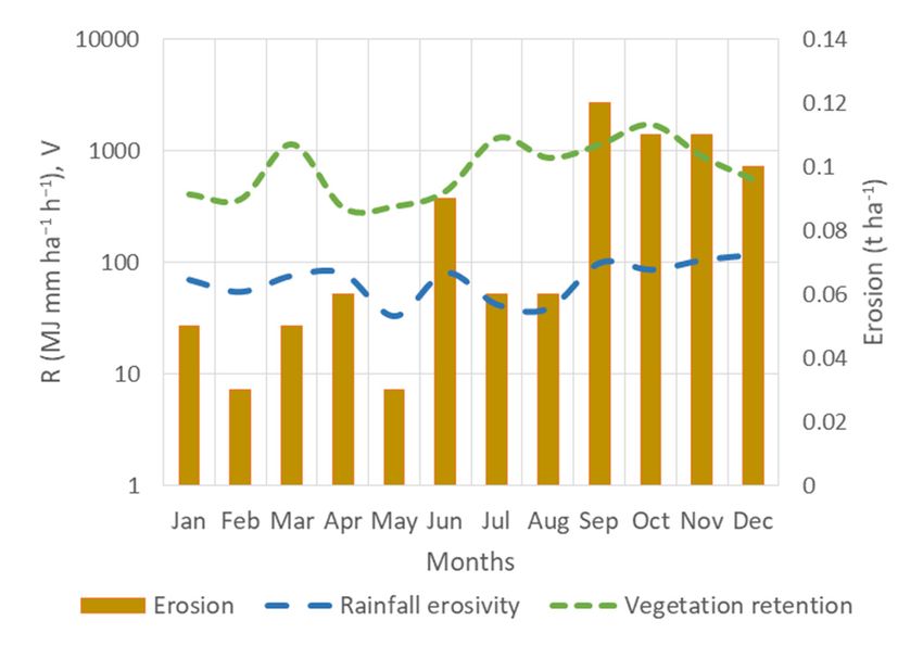
Geosciences 2020, 10, 89 15 of 22

 Figure 12. The annual erosion map for the Candelaro river basin.

 The mean annual soil loss rate derived with the G2 model for the area of Candelaro was found
to be 0.87 t ha−1. The maximum annual value was 210 t ha−1 and the minimum 0. The mean erosion
values per month were found to range from 0.03 t ha−1 for May up to 0.12 t ha−1 for September. The
very eastern and western parts of the basin show clearly to be more threatened by erosion than the
central parts. This could be attributed to the topographic nature of the basin (see Figure 9). In fact,
the central part of the basin is flat, in contrast to the sides, which are hilly or mountainous areas.
 In addition, the application of the G2 model in Candelaro made it possible to identify soil erosion
changes between months; thus, allowing seasonal comparisons. All months from September,
October, November, December, and June showed to be the most erosive months over the year. The
maximum erosion values per month were found to range from 6.69 t ha−1 for July up to 27.3 t ha−1 for
November (Table 4).

 Table 4. Statistics of monthly erosion (t ha-1) derived with the G2 model for the Candelaro river
 basin.

 Month Jan Feb Mar Apr May Jun
 Mean 0.05 0.03 0.05 0.06 0.03 0.09
 Std 0.21 0.18 0.26 0.24 0.10 0.30
 Max 12.7 16.8 12.3 17.6 7.3 21.2
 Month Jul Aug Sep Oct Nov Dec
 Mean 0.06 0.05 0.12 0.11 0.11 0.10
 Std 0.17 0.15 0.40 0.39 0.42 0.41
 Max 6.7 7.1 24.8 22.4 27.3 26.8

 The contribution of each month to the overall spatial distribution of erosion figures in the
Candelaro river basin was found generally equivalent in terms of magnitude, with only slight
differentiations. However, it seems to differ in spatial distribution; for example, in June, September,
November, and December, the mountainous areas show to have higher erosion values than the plains
(Figure 13). In general, the seasonal alterations showed to be affected mainly by rainfall erosivity
figures rather than vegetation or land use changes (Figure 14).

Geosciences 2020, 10, 89 16 of 22

 January February

 .

 March April

 May June

 July August

Geosciences 2020, 10, 89 17 of 22

 September October

 November December

 Figure 13. Monthly erosion maps for the Candelaro river basin (refer to the legend of Figure 12).

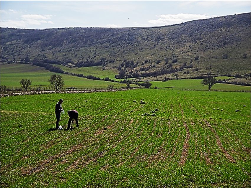
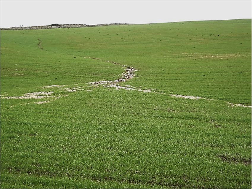
Geosciences 2020, 10, 89 18 of 22

 Figure 14. Mean monthly figures of rainfall erosivity and vegetation retention (left axis; logarithmic),
 vs. erosion (right axis; linear) for the Candelaro river basin.

5. Discussion
 The current study was the first erosion study in the area; thus, providing a reference for future
assessments. Soil erosion does not appear to be a major problem in the study area and quite limited
to some spots mostly in the sloping areas. However, erosion is still a problem, even if it concerns
limited areas (Figure 15).

 Figure 15. Erosion signs in a sloping cropland near Volturino, Province of Foggia (Photo credit: P.
 Zdruli).

 The riskiest land covers for erosion in the Candelaro river basin were found to be the lands
principally occupied by agriculture (CLC code 243), the olive groves (CLC code 223) and the burnt
areas (CLC code 334). The burnt areas were the riskiest land cover on an annual basis, with a value
of 3.90 t ha−1, and the monthly values varying from 0.42 t ha−1 in December to 0.57 t ha−1 in September.
However, the specific surfaces were very limited (0.88 Km2) in the Candelaro river basin during the
study period and moreover, they change rapidly over time. The agricultural-natural mixtures (CLC
code 243) show noticeable erosion risk figures (2.88 t ha−1), but they also keep a small share in the
land of Candelaro (28.3 Km2); this category revealed to contain the riskiest surfaces for most months
of the year. Finally, the olive groves show also noticeable values throughout the year, with an annual

Geosciences 2020, 10, 89 19 of 22

erosion rate of 2.04 t ha−1; at the same time, they occupy a significant part of Candelaro than the
previous two (100.5 Km2).
 On an annual basis, land covers in the Candelaro river basin, which demonstrate erosion risk
higher than the annual average (i.e., larger than 0.87 t ha−1) and at the same time cover a significant
surface (more than 5 Km2) include non-irrigated arable land (CLC code 211), olive groves (CLC code
223), natural grasslands (CLC code 321), sparsely vegetated areas (CLC code 333), small forested
surfaces, as well as other types of cropland. It is noticeable that one third of the olive groves, natural
grasslands, sclerophyllous vegetation surfaces, sparsely vegetated surfaces, and mixtures of cropland
with natural patches, half of the agricultural-natural mixtures, and almost one fifth of the arable land
are more erosive than the average on an annual basis (Table 5).

 Table 5. Extents for erosion rates higher than the annual erosion mean (0.87 t ha−1) per CORINE Land
 Cover category in the Candelaro river basin.

 Erosive % of the
 CORINE Land Cover category Erosive Extent (Km2)
 Class
 211 (Non-irrigated arable land) 282.5 18.1
 221 (Vineyards) 8.9 8.6
 223 (Olive groves) 37.2 36.7
 241 (Annual with permanent crops) 9.2 26.7
 242 (Complex cultivation patterns) 11.4 8.1
 243 (Agricultural-natural mixtures) 13.0 46.8
 311 (Broad-leaved forests) 8.8 13.0
 321 (Natural grasslands) 22.1 34.1
 323 (Sclerophyllous vegetation) 13.5 29.1
 333 (Sparsely vegetated areas) 21.5 34.7
 Total/Average 427.9 19.4

 The generally low erosion figures in the Candelaro basin derived with the current study seem
to differ from the moderate to high values (5–10 t ha−1) reported for the entire regional unit of Foggia
by the Joint Research Centre (reference year: 2010) [2]. However, this difference could be justified by
the fact that the two assessments have been conducted at completely different spatial and temporal
scales (i.e., the entire regional unit vs. only the Candelaro river basin; and annual vs. monthly
assessments). In addition to that, JRC’s assessment was focused only on agricultural lands, in contrast
to the current, which is generic for all existing land covers.
 For the first time, the G2 model was applied using a new satellite image type, namely Sentinel2,
concluding with an invention of a new alternative for estimating the V-factor. When there are not
cloud-free images for all months, weighted averaging of vegetation cover layers derived from the
available cloud-free Sentinel2 images can be computed for the missing months.

6. Conclusion
 In this research, the Candelaro river basin in Apulia region (Italy) was mapped for soil erosion
on a month-time interval, using the G2 model, in a Geographic Information System (GIS), and Remote
Sensing modelling framework. The study achieved to reveal the specific contribution of every land
cover to soil loss, especially regarding the seasonal changes of rain intensity and vegetation cover.
 The mean annual soil loss rate was found to be 0.87 t ha−1. The seasonal balance of erosion risk
was mainly for autumn months, but also for December and June. Burnt areas, mixed agricultural-
natural surfaces, and olive groves grown in the hills proved to be the riskiest land covers in the area.
Arable land was the most extensive land cover with erosion figures higher than the mean annual rate.
 Soil erosion is not a widespread problem in the study area. However, considering that in specific
locations, months, and land covers, erosion exceeds alarm rates (i.e., 10 t ha−1), the entire area should

Geosciences 2020, 10, 89 20 of 22

be put under careful monitoring, and emphasis should be given to sustainable land management
measures.
 With the rising number of available cloud-free Sentinel2 image scenes, the new alternative for
V-factor computation introduced in this study appears to be suitable for future erosion assessments
with G2, or other empirical models.
 One more time, the (now, revised) G2 model proved to work as a rapid, robust, and—at the same
time—flexible mapping tool. Moreover, it shows to be an appropriate solution for expanding erosion
assessments in the whole Apulia region.
Author Contributions: Conceptualization, C.K. and P.Z.; methodology, C.K.; software, C.K., O.B.; validation,
O.B., P.Z.; investigation, C.K., P.Z.; resources, P.Z, O.B.; data curation, C.K, O.B.; writing—original draft
preparation, C.K., O.B.; writing—review and editing, P.Z., O.B.; visualization, C.K.; supervision, P.Z.; project
administration, P.Z.; funding acquisition, P.Z. All authors have read and agreed to the published version of the
manuscript.

Funding: This research was funded by the CIHEAM Mediterranean Agronomic Institute of Bari in the context
of the Master Programme 2018–2019. Ouiza Bouarour received the title Master of Science under this programme.

Conflicts of Interest: The authors declare no conflict of interest.

References
1. Jones, R.J.; Le Bissonnais, Y.; Diaz, J.S.; Düwel, O.; Øygarden, L.; Prasuhn, P.B.V.; Yordanov, Y.; Strauss, P.;
 Rydell, B.; Uveges, J.B. Work Package 2: Nature and extent of soil erosion in Europe. Available online:
 https://citeseerx.ist.psu.edu/viewdoc/download?doi=10.1.1.486.3962&rep=rep1&type=pdf (accessed on 26
 February 2020)
2. Panagos, P.; Borrelli, P.; Poesen, J.; Ballabio, C.; Lugato, E.; Meusburger, K.; Montanarella, L.; Alewell, C.
 The new assessment of soil loss by water erosion in Europe. Environ. Sci. Policy. 2015, 54, 438–447,
 doi:10.1016/j.envsci.2015.08.012.
3. Panagos, P.; Karydas, C.G.; Gitas, I.Z.; Montanarella, L. Monthly soil erosion monitoring based on remotely
 sensed biophysical parameters: A case study in Strymonas river basin towards a functional pan-European
 service. Int. J. Digit. Earth 2012, 5, 461–487, doi:10.1080/17538947.2011.587897.
4. Kirkby, M.J.; Jones, R.J.; Irvine, B.; Gobin, A.; Govers, G.; Cerdan, O.; van Rompey, A.J.; Le Bissonnais, Y.;
 Daroussin, J.; King, D. Pan-European Soil Erosion Risk Assessment: The PESERA Map Belgium: European
 Communities. 2004. Available online:
 https://researchdirect.westernsydney.edu.au/islandora/object/uws:12030 (accessed on 26 February 2020)
5. Rubio, J.L.; Molina, M.J.; Andreu, V.; Gimeno-Garcia, E.; and Llinares, J.V.. Controlled forest fire
 experiments: Pre and postfire soil and vegetation patterns and processes. In Sustainable Use and Management
 of Soils in Arid and Semiarid Regions; Cano, A.F., Silla, R.O., Mermut, A.R., Eds.; Catena Verlag: Reiskirchen,
 Germany, 2005; pp 313–328.
6. Cerdà, A.; Hooke, J.; Romero-Diaz, A.; Montanarella, L.; Lavee, H. Soil erosion on Mediterranean Type-
 Ecosystems. Land Degrad. Dev. 2010, doi 10.1002/ldr.968.
7. Zdruli, P. Land resources of the Mediterranean: Status, pressures, trends and impacts on future regional
 development. Land Degrad. Dev. 2014, 25, 373–384, doi:10.1002/ldr.2150.
8. Piacentini, T.; Galli, A.; Marsala, V.; Miccadei, E. Analysis of Soil Erosion Induced by Heavy Rainfall: A
 Case Study from the NE Abruzzo Hills Area in Central Italy. Water 2018, 10, 1314.
9. OECD. Enevironmental Performance of Agriculture in OECD Countries Since 1990; OECD Publishing: Paris,
 France, 2008.
10. Rendell, H.M. Soil Erosion and Land Degradation in Southern Italy. In Desertification in Europe; Springer:
 Dordrecht, The Netherlands, 1986.
11. Dazzi, C.; Lo Papa, G. Soil threats. In The Soils of Italy; World Soil Book Series; Costantini, D., Ed.; Springer
 Science+Business Media: Dordrecht, The Netherlands, 2013; doi:10.1007/978-94-007-5642-7_8.
12. APAT. Rapporto sulle frane in Italia. In II progetto IFFI. Rapporti APAT 78/2007; 2007; ISBN:978-88-448-0310-
 0. Available online: http://www.isprambiente.gov.it/it/pubblicazioni/rapporti/Rapporto-sulle-frane-in-
 Italia (accessed on 26 February 2020)
13. Zanchi, C. Soil loss and seasonal variation of erodibility in two soils with different texture in the Mugello
 valley in Central Italy. Catena Suppl. 1988, 12, 167–174.

Geosciences 2020, 10, 89 21 of 22

14. Van der Knijff, J.M.; Jones, R.J.A.; Montanarella, L. Soil erosion risk assessment in Italy (JRC Scientific and
 Technical Report, EUR 19044 EN). Available online:
 https://esdac.jrc.ec.europa.eu/ESDB_Archive/serae/GRIMM/italia/eritaly.pdf (accessed on 26 February
 2020)
15. Vacca, A.; Loddo, S.; Ollesch, G.; Puddu, R.; Serra, G.; Tomasi, D.; Aru, A. Measurement of runoff and soil
 erosion in three areas under different land use in Sardinia (Italy). Catena 2000, 40, 69–92, doi:10.1016/S0341-
 8162(00)00088-6.
16. Van Rompaey, A.J.J.; Bazzoffi, P.; Jones, R.J.A.; Montanerella, L.; Govers, G. Validation of soil erosion risk
 assessments in Italy. In European Soil Bureau Research Report No. 12, EUR 20676 EN.; Office for Official
 Publications of the European Communities: Luxembourg, 2003; p 25.
17. Bagarello, V.; Ferro, V. Analysis of soil loss data from plots of differing length for the Sparacia experimental
 area, Sicily, Italy. Biosyst. Eng. 2010, 105, 411–422, doi:10.1016/j.biosystemseng.2009.12.015.
18. Märker, M.; Angeli, L.; Bottai, L.; Costantini, R.; Ferrari, R.; Innocenti, L.; Siciliano, G. Assessment of land
 degradation susceptibility by scenario analysis: A case study in Southern Tuscany, Italy. Geomorphology
 2008, 93, 120–129, doi:10.1016/j.geomorph.2006.12.020.
19. Borselli, L.; Cassi, P.; Torri, D. Prolegomena to sediment and flow connectivity in the landscape: A GIS and
 field numerical assessment. Catena 2008, 75, 268–277, doi:10.1016/j.catena.2008.07.006.
20. Della Seta, M.; Del Monte, M.; Fredi, P.; Lupia Palmieri, E. Space–time variability of denudation rates at the
 catchment and hillslope scales on the Tyrrhenian side of Central Italy. Geomorphology 2009, 107, 161–177,
 doi:10.1016/j.geomorph.2008.12.004.
21. Terranova, O.; Antronico, L.; Coscarelli, R.; Iaquinta, P. Soil erosion risk scenarios in the Mediterranean
 environment using RUSLE and GIS: An application model for Calabria (southern Italy). Geomorphology
 2009, 112, 228–245, doi:10.1016/j.geomorph.2009.06.009.
22. Torri, D.; Santi, E.; Marignani, M.; Rossi, M.; Borselli, L.; Maccherini, S. The recurring cycles of biancana
 badlands: Erosion, vegetation and human impact. Catena 2013, 106, 22–30, doi:10.1016/j.catena.2012.07.001.
23. Grimm, M.; Jones, R.J.A.; Rusco, E.; Montanarella, L. Soil erosion risk in Italy: A review USLE approach. In
 European Soil Bureau Research Report No. 11, EUR 20677 EN.; Office for Official Publications of the European
 Communities: Luxembourg, 2003; p. 28.
24. Costantini, E.A.; Lorenzetti, R. Soil degradation processes in the Italian agricultural and forest ecosystems.
 Ital. J. Agron. 2013, 8, e28, doi:10.4081/ija.2013.e28.
25. Zdruli, P.; Karydas, C.G.; Dedaj, K.; Salillari, I.; Cela, F.; Lushaj, S.; Panagos, P. High resolution
 spatiotemporal analysis of erosion risk per land cover category in Korçe region, Albania. Earth Sci. Inform.
 2016, 9, 481–495, doi:10.1007/s12145-016-0269-z.
26. Karydas, C.G.; Panagos, P. The G2 erosion model: An algorithm for month-time step assessments. Environ.
 Res. 2018, 161, 256–267, doi:10.1016/j.envres.2017.11.010.
27. Wischmeier, W.H.; Smith, D.D. Predicting rainfall erosion losses-a guide to conservation planning. In
 Predicting Rainfall Erosion Losses-A Guide to Conservation Planning; Purdue University: West Lafayette, IN,
 USA, 1978.
28. Renard, K.G.; Foster, G.R.; Weesies, G.A.; McCool, D.K.; Yoder, D.C. Predicting Soil Erosion by Water: A Guide
 to Conservation Planning with the Revised Universal Soil Loss Equation (RUSLE). United States Department of
 Agriculture: Washington, DC, USA, 1997.
29. Ferro, V. Deducing the USLE mathematical structure by dimensional analysis and self-similarity theory.
 Biosyst. Eng. 2010, 106, 216–220.
30. CORDIS, Geoland2 -Towards An Operational GMES Land Monitoring Core Service (2008–2012). Available
 online: https://cordis.europa.eu/project/id/218795 (accessed on 20 August 2019).
31. Karydas, C.G.; Panagos, P. Modelling monthly soil losses and sediment yields in Cyprus. Int. J. Digit. Earth
 2016, 9, 766–787, doi:10.1080/17538947.2016.1156776.
32. Halecki, W.; Kruk, E.; Ryczek, M. Evaluation of water erosion at a mountain catchment in Poland using the
 G2 model. Catena 2018, 164, 116–124, ISSN 0341-8162, doi:10.1016/j.catena.2018.01.014.
33. European Soil Data Centre (ESDAC) of the Joint Research Centre (JRC). Available online:
 https://esdac.jrc.ec.europa.eu/themes/g2-model (accessed on 20 August 2019).
34. Land Copernicus, BIOPAR products. Available online: http//land.copernicus.eu/global/products (accessed
 on 20 August 2019).

Geosciences 2020, 10, 89 22 of 22

35. Torma, M.; Hatunen, S.; Harma, P.; Jarvenpaa, E. (2012). Sentinel2 Images and Finnish CORINE Land Cover
 Classification. In Proceedings of the First Sentinel2 Preparatory Symposium, Frascati, Italy, 23–27 April
 2012.
36. European Space Agency (ESA). (2012, 2018). Available online: https://www.esa.int/ESA (accessed on 20
 August 2019).
37. Lo Presti, R.; Barca, E.; Passarella, G. A methodology for treating missing data applied to daily rainfall data
 in the Candelaro River Basin (Italy). Environ. Monit. Assess. 2010, 160, 1–22, doi:10.1007/s10661-008-0653-3.
38. Steduto, P.; Todorovic, M. The agro-ecological characterization of Apulia region (Italy): Methodology and
 experience. In Soil Resources of Southern and Eastern Mediterranean Countries Options Méditerranéennes, SERIE
 B: Studies and Research, No. 34; Zdruli, P., Steduto, P., Lacirignola, C., Montanarella, L., Eds.; CIHEAM:
 Paris, France, 2001; pp. 143–158.
39. De Girolamo, A.M.; Lo Porto, A.; Pappagallo, G.; Tzoraki, O.; Gallart, F. The Hydrological Status Concept:
 Application at a Temporary River (Candelaro, Italy). River Res. Appl. 2015, 31, 892–903, doi:10.1002/rra.2786.
40. Caliandro, A.; Lamaddalena, N.; Stelluti, M.; and Steduto, P. Progetto ACLA2 Caratterizzazione
 agroecologica della Regione Puglia in funzione della potenzialità produttiva. In Technical Report, P.O.P.
 Puglia 94–99; Mediterranean Agronomic Institute of Bari and the University of Bari: Bari, Italy, 2005.
41. Copernicus, Scientific Hub, Sentinel2. Available online: https://scihub.copernicus.eu/dhus/#/home
 (accessed on 20 August 2019).
42. Copernicus, CORINE Land Use. Available online: http://land.copernicus.eu/pan-european/corine-land-
 cover (accessed on 20 August 2019).
43. Jetten, V.; De Roo, A.D.; Favis-Mortlock, D. Evaluation of field-scale and catchment-scale soil erosion
 models. Catena 1999, 37, 521–541, doi:10.1016/S0341-8162(99)00037-5.
44. Longley, P.A.; Goodchild, M.F.; Maguire, D.J.; Rhind, D.W. Geographic Information Systems and Science; John
 Wiley & Sons: Hoboken, NJ, USA, 2004.
45. Brown, L.C.; Foster, G.R. Storm erosivity using idealized intensity distributions. Trans. ASAE 1987, 30, 379–
 386, doi:10.13031/2013.31957.
46. Baret, F.; Weiss, M.; Lacaze, R.; Camacho, F.; Makhmara, H.; Pacholcyzk, P.; Smets, B. GEOV1: LAI and
 FAPAR essential climate variables and FCOVER global time series capitalizing over existing products.
 Part1: Principles of development and production. Remote Sens. Environ. 2013, 137, 299–309,
 doi:10.1016/j.rse.2012.12.027.
47. Karydas, C.G.; Gitas, I.Z.; Koutsogiannaki, E.; Lydakis-Simantiris, N.; Silleos, G.N. Evaluation of spatial
 interpolation techniques for mapping agricultural topsoil properties in Crete. EARSeL eProceedings 2009, 8,
 26–39.
48. Moore, I.D.; Burch, G.J. Physical basis of the length-slope factor in the universal soil loss equation 1. Soil
 Sci. Soc. Am. J. 1986, 50, 1294–1298, doi:10.2136/sssaj1986.03615995005000050042x.
49. Moore, I.D.; Wilson, J.P. Length-slope factors for the Revised Universal Soil Loss Equation: Simplified
 method of estimation. J. Soil Water Conserv. 1992, 47, 423–428.
50. Desmet, P.; Govers, G.; A GIS procedure for automatically calculating the USLE LS factor on
 topographically complex landscape units. J. Soil Water Conserv. 1996, 51, 427–433.
51. Panagos, P.; Karydas, C.; Ballabio, C.; Gitas, I. Seasonal monitoring of soil erosion at regional scale: An
 application of the G2 model in Crete focusing on agricultural land uses. Int. J. Appl. Earth Obs. Geoinf. 2014,
 27, 147–155.

 © 2020 by the authors. Licensee MDPI, Basel, Switzerland. This article is an open access
 article distributed under the terms and conditions of the Creative Commons Attribution
 (CC BY) license (http://creativecommons.org/licenses/by/4.0/).