Contribution of bone-reverberated waves to sound localization of dolphins: A numerical model
←
→
Page content transcription
If your browser does not render page correctly, please read the page content below
Acta Acustica 2021, 5, 3
Ó A. Hejazi Nooghabi et al., Published by EDP Sciences, 2020
https://doi.org/10.1051/aacus/2020030

                                                                                                                        Available online at:
                                                                                                         https://acta-acustica.edpsciences.org

    SCIENTIFIC ARTICLE

Contribution of bone-reverberated waves to sound localization
of dolphins: A numerical model
Aida Hejazi Nooghabi1,2,*, Quentin Grimal2, Anthony Herrel3, Michael Reinwald4,5, and Lapo Boschi1,6,7
1
  Sorbonne Université, CNRS-INSU, Institut des Sciences de la Terre Paris, ISTeP UMR 7193, 75005 Paris, France
2
  Sorbonne Université, Laboratoire d’Imagerie Biomédicale (LIB),CNRS 7371 – INSERM 1146, 75006 Paris, France
3
  UMR 7179 C.N.R.S/M.N.H.N., Bâtiment d’Anatomie Comparée, 75005 Paris, France
4
  Department of Biomedical Engineering, School of Biomedical Engineering and Imaging Sciences, King’s College London, WC2R 2LS
  London, UK
5
  Department of Zoology, University of Oxford, OX1 2JD Oxford, UK
6
  Dipartimento di Geoscienze, Università degli Studi di Padova, 35122 Padova, Italy
7
  INGV Istituto Nazionale di Geofisica e Vulcanologia, Via Donato Creti, 12, 40100 Bologna, Italy

            Received 5 May 2020, Accepted 2 December 2020

            Abstract – We implement a new algorithm to model acoustic wave propagation through and around a dolphin
            skull, using the k-Wave software package [1]. The equation of motion is integrated numerically in a complex
            three-dimensional structure via a pseudospectral scheme which, importantly, accounts for lateral hetero-
            geneities in the mechanical properties of bone. Modeling wave propagation in the skull of dolphins contributes
            to our understanding of how their sound localization and echolocation mechanisms work. Dolphins are known
            to be highly effective at localizing sound sources; in particular, they have been shown to be equally sensitive to
            changes in the elevation and azimuth of the sound source, while other studied species, e.g. humans, are much
            more sensitive to the latter than to the former. A laboratory experiment conducted by our team on a dry skull
            [2] has shown that sound reverberated in bones could possibly play an important role in enhancing localization
            accuracy, and it has been speculated that the dolphin sound localization system could somehow rely on the
            analysis of this information. We employ our new numerical model to simulate the response of the same skull
            used by [2] to sound sources at a wide and dense set of locations on the vertical plane. This work is the first
            step towards the implementation of a new tool for modeling source (echo)location in dolphins; in future work,
            this will allow us to effectively explore a wide variety of emitted signals and anatomical features.

            Keywords: Dolphin’s echolocation, Numerical modeling, Reverberation, Correlation

1 Introduction                                                              depending on the direction it comes from; these differences
                                                                            are summarized in the “head-related transfer function”
    Most literature concerned with the evolution of sound                   (HRTF). Behavioural experiments on humans suggest that
localization postulates that this task is accomplished by                   each individual unconsciously learns to use its HRTF to
means of several well established auditory cues, at least in                localize sounds [5]. It is generally accepted that, in practice,
mammals [3, 4]. Firstly, the binaural or interaural time-                   the auditory system is very sensitive to certain prominent
or phase-difference (ITD or IPD): the delay between the                     peaks and notches of the frequency spectrum perceived by
arrival time of a sound at the two ears. Secondly, the binau-               the ears, or “spectral cues”, whose amplitude and location
ral or interaural intensity or level difference (IID or ILD):               along the frequency axis, controlled by the complex shape
the difference in the intensity of a sound, as perceived at                 of the pinnae, depend on the elevation of the source; a num-
the two ears. The locus of sources that can be associated                   ber of studies have shown that up-down and front-back
to a given ITD and/or ILD is a cone, sometimes dubbed                       ambiguities are dealt with based on such spectral cues [4, 6].
the “cone of confusion” [4]. Since humans and other species                     The ITD/ILD/spectral-cue model has been successfully
are known to distinguish different sources within such a                    applied to explain the results of behavioural experiments,
cone, a third psychoacoustic cue must exist. In fact, it is                 and has found neurophysiological and neuroanatomical
clear from the physics of acoustic-wave propagation that                    support across different species [4, 7]. At least in the case
the same signal interacts differently with our anatomy                      of humans, it has also been shown to have limitations that
*Corresponding author: aida.hejazi_nooghabi@upmc.fr                         can be predicted theoretically and are confirmed by
This is an Open Access article distributed under the terms of the Creative Commons Attribution License (https://creativecommons.org/licenses/by/4.0),
              which permits unrestricted use, distribution, and reproduction in any medium, provided the original work is properly cited.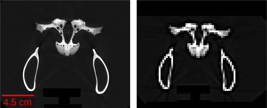
2                                    A. Hejazi Nooghabi et al.: Acta Acustica 2021, 5, 3

behavioural experiments. Namely, (i) since binaural cues           important heterogeneity within the bone. Based on grays-
play a fundamental role, subjects that are deaf on one side        cale values, we define a model of the skull’s mechanical
can be expected and are indeed observed to perform poorly          properties, and numerically simulate elastic wave propaga-
in sound localization tasks [4]; (ii) normal-hearing subjects      tion through it via a pseudospectral scheme [1]. Impor-
fail at determining the correct elevation of narrow-band           tantly, bone heterogeneity, neglected in other similarly-
sources: elevation is determined through the identification         minded numerical studies (e.g. [17, 18]) is accounted for
of spectral peaks and notches, which requires that the emit-       in our simulations. While it is impossible (for a number of
ted sound be broadband [8, 9]; (iii) because spectral cues are     technical reasons that we discuss) to reproduce Reinwald
not as accurate as ITD and ILD, at least humans have been          et al.’s [2] experiment exactly, our results share all the
observed to be less sensitive to changes in source elevation       important features of their data.
than azimuth: according to experiments, their minimum
audible angle (MAA, or the smallest detectable angular dif-
ference between the locations of two identical sources of          2 Method
sound) for sources within the vertical plane is never less
than 4°, vs. ~ 1° on the horizontal plane [10].                       In this section, we introduce the numerical tool we
    Behavioural experiments indicate that odontocete ceta-         employed; we explain how we built a model of the skull’s
ceans, which rely on sound and on their biosonar to carry          mechanical properties based on a computed tomography
out many essential tasks, do not suffer from (some of) the         scan and we describe the configuration of our numerical
mentioned limitations. They are known to emit high-                experiment.
frequency clicks and burst-pulsed calls as well as lower fre-
quency whistles. For example, the frequency range of               2.1 Numerical simulation toolbox
echolocation signals emitted by short-beaked common dol-
phins is between 23 and 67 kHz [11]. Despite the absence              We treat the skull as a purely elastic medium and model
of pinnae, bottlenose dolphins have been shown to be               wave propagation via k-Wave1, an open-source toolbox
equally sensitive to changes in the elevation or azimuth of        which solves the coupled first-order equations [1]:

signals similar to their echolocation clicks [12, 13]; they have                orij        ovk       ovi ovj
also been shown to respond to clicks with a MAA of 0.7°,                             ¼ kdij     þl        þ      ;        ð1Þ
                                                                                 ot         oxk       oxj oxi
superior to the localization accuracy of other studied mam-
mals [3]. It has been suggested [14] that these results cannot
be explained without invoking, within the auditory system
of dolphins, a localization mechanism different from the                                   ovi 1 orij
                                                                                              ¼       ;                   ð2Þ
ITD/ILD/spectral-cue model attributed to other species.                                    ot   q oxj
    An essential factor in assessing this speculation is the
analysis of the dolphins’ HRTF, and the information it             where r denotes stress, v particle velocity, and the Ein-
might carry pertaining to source location. In an earlier           stein summation notation is adopted. k and l are the
study [15], our team has tackled this problem with an exper-       Lamé parameters and q is the mass density. The compres-
imental approach, recording and analyzing mechanical               sional and shear wave speed (a and b, respectively) are,
waves propagating through a dolphin skull. Their experi-                              sffiffiffiffiffiffiffiffiffiffiffiffiffiffi      rffiffiffi
ments were performed using two different signals: a nar-                                 k þ 2l             l
                                                                                   a¼                 ; b¼      :        ð3Þ
row-band chirp and a sinusoidal burst, both with a                                          q               q
central frequency of 45 kHz. Reinwald [15] concluded that
the skull shape and structure does not give rise to promi-         Equations (1) and (2) are solved for an elastic isotropic
nent, location-dependent features in the HRTF spectrum;            medium using the Fourier pseudospectral method. The lat-
they found, on the other hand, that the skull transfer func-       ter is based on the Fourier collocation spectral method for
tion contains sufficient information for sources to be pre-         computing spatial derivatives and the finite difference
cisely localized by an algorithm based on Pearson’s                method for time integration [1, 19].
correlation, equivalent to the so-called “time-reversal”
scheme postulated by Catheline et al. [16].                        2.2 Model of dolphin’s skull
    The frequency band of Reinwald et al.’s [2] data was
severely limited by their experimental setup; additionally,            The flawless skull of a young adult short-beaked com-
it would be very difficult, if possible at all, to carry out sim-   mon dolphin (Delphinus delphis) of ~50 cm length and
ilar experiments on full heads, including soft tissues: yet,       ~20 cm width, was scanned at the AST-RX X-ray tomogra-
soft tissues might have a non-negligible impact on the             phy platform at the National Museum of Natural History in
HRTF and thus on localization. We here accordingly                 Paris, using a v|tome|x L 240-180 industrial micro CT scan-
develop a model of elastic-wave propagation through a dol-         ner with voltage = 150 kV, current = 310 lA and exposure
phin head, and validate it by application on the same skull        time of 333 ms. Data were reconstructed using the datos|x
that was employed in the Reinwald et al. [2] experiments.          software and exported into 4106 slices of 16-bit TIFF
We obtain high-resolution (voxel size = 111 lm) X-ray              images in coronal view. The resulting images are in
                                                                   1
tomography images of the skull resolving small but possibly            http://www.k-wave.org/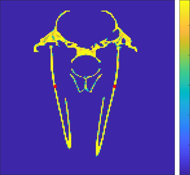
A. Hejazi Nooghabi et al.: Acta Acustica 2021, 5, 3                                                           3

                                                                          Figure 2. Three slices of dolphin’s skull, where we define the
Figure 1. A slice of the CT scan images illustrating the                  trabecular and cortical bones.
mandible and teeth at the original voxel size (left) and the
dowsampled processed image (right).
                                                                              We next associate a value for the mass density and wave
grayscale which is representative of the mean attenuation of              speed to each voxel. We convert the images from 16-bit to
X-rays at each voxel. Their voxel size is 111 lm along x, y               8-bit, so that the gray scale values range from 0 to 255. We
and z directions, which is large compared to the grid size                apply a self-calibration on CT values, so that the brighter
envisaged for our simulations. We hence downsampled the                   regions are assigned higher values of mass density and wave
images. Voxel size is an important parameter as it defines                 speed compared to the darker regions with lower CT values.
the spatial grid size in the simulations. Moreover, decreas-              We set mass density to vary from 1001 to 2000 kg/m3 with
ing the resolution implies loss in the information on the                 255 equal increments. Next, based on the density associated
structure. The gray values are important because they are                 to each voxel, the voxel-wise values of a and b are calcu-
the basis for associating elastic parameters to each voxel.               lated based on Equations (4) and (5), respectively. The
This image processing step demands a compromise between                   value of 0.3 was used for the Poisson ratio (m) [20]:
the computational cost of the simulations and the degree of
information on the physical structure of the skull that                                 a ¼ 0:004q2 þ 14:9q  10664;                           ð4Þ
should be kept. In Figure 1 we show a slice with the original                                      sffiffiffiffiffiffiffiffiffiffiffiffiffiffiffiffiffi
voxel size (i.e., 111 lm) and the 20-times increased voxel                                            1  2m
size (i.e. 2220 lm).                                                                           b¼a                    :                         ð5Þ
                                                                                                    2ð1  mÞ
    We chose to implement this level of resolution, as a good
compromise between accuracy and computational cost,
after a suite of simulations on two-dimensional structures                Equation (4) was obtained by fitting to experimental data
of comparable complexity; these tests showed that signals                 (compressional wave speed and mass density for human
modeled at the receiver locations were not modified signifi-                cortical bone samples). This data was obtained as described
cantly by changes in numerical grid spacing (See Appendix                 in [21]. Based on the Resonant Ultrasound Spectroscopy
A for more details). Downsampling blurs the images and                    (RUS) method, anisotropic velocities are measured for
hence some detailed information on the structure is lost.                 cuboid specimens. As resonant frequencies are directly
For example, the distinction between the trabecular and                   related to the dimension of the sample and the wave speed
cortical bone becomes less obvious. These two main parts                  inside it, RUS provides values for anisotropic velocities
of the bone structure are shown for different slices with                 independent of density measurements.
the original resolution in Figure 2.                                          Figure 3 shows the map of the wave speeds for the same
    Also, the gray scale values vary from the original ones.              slice shown in Figure 1. Considering that the background
It should be noted that the processed image here has been                 medium is water with a = 1500 m/s and b = 0, the mini-
sharpened in order to magnify the contrast of the gray val-               mum and maximum values for the compressional wave
ues in the downsampled image and all the image processing                 speed in these maps are 1500 m/s and 3861 m/s and the
steps have been performed using ImageJ software.                          corresponding values for b are 0 m/s and 2919 m/s.

                        (a)                                                            (b)

                                                3500                                                                  2500
                                                       wave speed (m/s)

                                                                                                                             wave speed (m/s)
                                                        compressional

                                                                                                                      2000
                                                3000
                                                                                                                                   shear

                                                                                                                      1500
                                                2500
                                                                                                                      1000
                                                2000
                                                                                                                      500

                                                1500                                                                  0

Figure 3. (a) Compressional and (b) shear wave speed values for a slice of the computed tomography scan in a water background.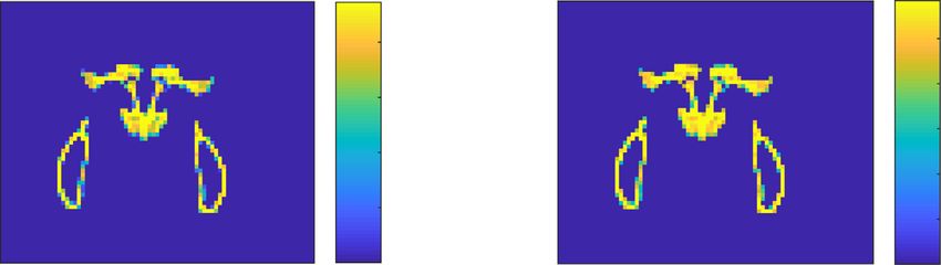
4                                            A. Hejazi Nooghabi et al.: Acta Acustica 2021, 5, 3

            1
Amplitude

            0

            -1
                 0   0.05   0.1     0.15         0.2     0.25     0.3
                                  time(ms)

Figure 4. Signal (“sinusoidal burst”) emitted by sources in
numerical simulations.

2.3 Numerical set-up

    In the experiment performed by [2], the skull is
immersed in water far from the walls and floor of the pool,
and is illuminated by sources along different elevations. The
acceleration is measured using accelerometers attached to
the posterior part of the mandible. In order to be close to
the experimental set-up in [2] and since one of the goals
of this study is to investigate the mechanism by virtue of
which the elevation of a sound source is determined, in                 Figure 5. Simulation configuration. The solid curve marks the
the following we shall position numerical sources on the me-            range of elevation of the sources. From each elevation, a plane
                                                                        wave is emitted.
dian plane (the hypothetical plane that divides the head
into left and right), at a range of different elevations. In
practice, we illuminate the skull with a plane wave whose
wave vector varies from 0° to 90°. Angle zero corresponds               in computational cost. We therefore adopt another
to the wave coming from the front of the skull while angle              approach here assuming that a plane wave already formed
90 corresponds to the wave coming from above it.                        outside the simulation box, we consider the points located
    The input signal is a sinusoidal burst with the central             on the edges of the simulation domain as point sources, each
frequency of 45 kHz and total duration of 100 ls as shown               emitting the same signal with a previously-calculated delay.
in Figure 4.                                                            By firing an identical signal with the proper time delay from
    Our simulation domain consists of a box of 0.3 m by                 neighboring points, we ensure the formation of a plane wave
0.8 m by 0.7 m with the spatial grid size of 2.22 mm in                 front which in contrast to the point-source approach does
all three directions which ensures a minimum number of                  not require a large simulation box. The source mask in
20 points per wavelength. The total number of grid points               3D is two perpendicular planes at the edge of the simulation
are 135 by 360 by 315. In order to guarantee the stability              box where each point on these planes acts as a source.
of the simulations, based on the Courant–Friedrichs–Lewy                    We record signals inside the pan bone (i.e. the thin pos-
                                        t
stability criterion [19], we select c0 x  = 0.1, where Dt and          terior end of the lower jaw bone) on either side of the mand-
Dx are the temporal and spatial steps, respectively. The                ible. The exact locations of receivers were not recorded
value of 0.1 was chosen after careful trial and error; this             when conducting the analogue experiment [2], but the dis-
value, sensibly smaller than 1, is compatible with example              tance between receivers was: in our simulations, receivers
values suggested in the k-Wave documentation. Our numer-                were positioned as similar to the experiment as possible,
ical configuration is shown in Figure 5.                                 based on this datum and on several available photos of
    Once the elastic parameters and the numerical proper-               the experimental set-up. A 2D view of the position of the
ties are determined, we illuminate the skull by a plane                 receivers is shown in Figure 6.
wave. This is equivalent to limiting our application to                     The receivers are positioned on the bone with identical
sources or echolocation targets that are not in the immedi-             elastic properties on each side and they measure velocity
ate vicinity of the subject. It is important to note that we do         of oscillation along x, y and z directions. Each simulation
not intend to model the actual acoustical environment of                takes approximately 24 h on CPUs of type Inter(R)
the dolphin, but to characterize its localization abilities.            Xenon(R) CPU E5-2695 v3.
This is usually done by considering sound coming from dif-
ferent directions, i.e., the angle of the incoming wave should
be clearly defined. Plane waves are better suited for this               3 Results
goal, since they have a unique and well-defined direction
of propagation.                                                             In this section, we show the results pertaining to the
    In order to numerically generate a plane wave, one                  validity of our model through different sets of comparisons
might deploy a point source in the far field of the object,              with the experimental case; namely as direct comparison of
but this approach requires a large enough simulation box                the signals, measurement of the inter-receiver time differ-
to satisfy the far field condition, i.e. a significant increase           ence and correlation maps.
A. Hejazi Nooghabi et al.: Acta Acustica 2021, 5, 3 5
2500
2000
shear wave speed (m/s)
1500
1000
500
0
Figure 6. Receiver positions shown by red full circles on a slice
of the skull with values of shear wave speed. The background
material is water.
3.1 Waveform comparison
Figure 7. Comparison of the acceleration signals recorded in
We adopt different criteria to validate the reliability of the experiment (black) and the simulation (blue) for a source
elevation of 25° (a) with the normalized amplitude and (b) with
our numerical model of the skull. In all cases, we use data
the scaled normalized amplitude. Dashed and solid arrows mark
from the mentioned laboratory experiment conducted by the direct arrival and coda windows, respectively.
our team on the same skull [2]. In this experiment, the skull
was immersed in water, centered in depth and width inside
a water tank and illuminated from different angles on the
vertical plane using a broadband marine transducer. The
input signal in the simulation and experimental case are
the same (Fig. 4). The receivers in the experiment are
accelerometers. The position of the receivers in simulations
is very close to the ones implemented in the experiment
with a maximum difference of ~5 mm. In contrast to the
experiment where data are available for a range of angles
varying from 90° to 90°, we have data for the range of
0°–90°.
As a first proxy, we directly compare the experimentally Figure 8. Comparison of the experimentally recorded (black)
recorded signals with their numerically computed counter- and numerically simulated (blue) acceleration, for source eleva-
parts. In the latter case, acceleration is computed from tion of 82°. The amplitude of the reverberated part of the
velocity by numerical differentiation, and only the x compo- experimental data is scaled as in Figure 7b.
nent, which is normal to the mandible and pointing out-
wards from it, is considered (Fig. 5). This component is
the closest one to what is measured in the experiment. experimental signal and show the resulting waveforms in
Compared to the input signal in Figure 4, the recorded sig- Figure 7b. Amplitudes are scaled assuming an exponential
nals (in both experiment and simulation) are perturbed, decay of the signal with time (t), as is commonly done in
due to the interference of the incoming wave with the medical ultrasound imaging. This technique, called time
bone-reverberated one. Because wave propagation is faster gain compensation (TGC), assumes an exponential decay
in bone than in water, reverberated signal arrives almost of the signals as they penetrate into the attenuating tissue.
as early as the direct one, and cannot be easily separated In order to retrieve the lost energy by time, the amplitude is
from it by visual analysis. This phenomenon can be more multiplied by exp(at). In our case, the value of a is chosen
or less prominent depending on the angle of incidence. As by trial and error.
an example, in Figure 7a, we show the comparison between The consistency between the simulated and experimen-
the experimental and simulation data for the left receiver tal signals becomes less clear for some angles. The worst
and an incoming angle of 25°. case of the observed vs. simulated waveform decorrelation
Figure 7 shows that experimental and numerical signals is shown in Figure 8. In this case, the codas of the two sig-
are most often in phase with one another (this is true for nals are not in phase, but, again, the envelope of the rever-
both the direct and reverberated signal); the amplitude of berated wavefield is captured fairly well. Simulated and
experimental data is, however, strongly attenuated, while experimental data for both left and right receivers are com-
attenuation has been neglected in simulations. In order to pared in Appendix B for a suite of different elevations of the
facilitate the comparison, we scale the amplitude of the source.6 A. Hejazi Nooghabi et al.: Acta Acustica 2021, 5, 3
with unique target locations. The dolphin would then locate
the source of the perceived click at the location correspond-
ing to the stored echo that, of all those available in the
library, is best correlated with it. In this case, we have
two receivers but localization based on correlation is still
possible thanks to the presence of a complex structure i.e.
the skull. This is equivalent to what has previously been
shown in time reversal experiments [22]. We quantify the
effectiveness of this algorithm by using signals resulting
Figure 9. Comparison of the time difference between the from our simulations. This allows us to identify the contri-
signals received at the left and right receivers obtained from the bution of different parts of the signal to localization.
experimental (red) and simulation (blue) data. Uncertainty of Pearson’s correlation [23] is used as a quantitative mea-
the experimental values is around 5 ls. sure of similarity. In practice, our algorithm first aligns a
pair of signals based on the first (non reverberated) arrival,
similar to a “normal moveout” correction in seismics [24].
3.2 ITD The correlation of the so aligned traces is then computed,
summing over the sample by sample product of the two sig-
The second criterion for validating our numerical model nals. We then normalize the correlation value by the square
is the time difference between the signals recorded at the root of the product of the energy of the two signals as
left and right receivers. Assuming that the skull is symmet- follows,
ric, the interaural time difference (ITD) between the two Pt¼tf 0
received signals from the sources located on the median t¼ti s1 ðt Þs2 ðtÞ
C ¼ qffiffiffiffiffiffiffiffiffiffiffiffiffiffiffiffiffiffiffiffiffiffi
Pt¼tf q ffiffiffiffiffiffiffiffiffiffiffiffiffiffiffiffiffiffiffiffiffiffi
Pt¼tf 0 2 ; ð6Þ
plane is expected to be zero. However, the dolphin skull is
not symmetric. Here, we compare the values of ITD for sim- t¼ti s 1 ð t Þ2
t¼ti 2s ðtÞ
ulated and experimental signals. We find the ITD by taking
the difference between the arrival time of the first peak in where s1(t) is a signal received at a given receiver from a
0
the signals recorded at the left and right receivers. This arri- given angle and s2 ðtÞ is the delayed version of s2(t) which
val time was first identified automatically, as the time when could be any of the signals received at the same receiver
signal amplitude would exceed a selected threshold, and from all other angles [23].
subsequently checked visually by the first author of this We prefer the combination of moveout and correlation
article. This approach is applied to both simulation and rather than simple cross-correlation, because we have
experimental data, and the ITD versus the incidence angle neglected the attenuation in our simulations. This results
for both cases is shown in Figure 9. in relatively large-amplitude reverberations, which might
As can be seen, the variations of ITD values obtained cause cross-correlation to be amplitude-biased. Conse-
from our simulations show the same overall “bias” as the quently, the maximum of the cross-correlation which is
experimental data, but with elevation-dependent fluctua- expected to be the maximum of the similarity could be
tions that are less-reproduced compared to the experimen- biased.
tal case. Furthermore, an increasing trend from 0° to 20° After aligning the signals, we explore two different
is observed in the simulation data but it is not as sharp approaches:
as the experimental case. It should be noted that the orien-
tation of the incoming wavefront with respect to the skull in We correlate only the direct part of the signals. Direct
the experimental case is not as accurately-defined as in the waves are those part of the signals that mimic the
simulations. Therefore, there might be an error in the direc- form of the incident wave that has not undergone
tion of the incident wave as recorded by the experimenters any reverberations (see Fig. 7b for distinction between
in [2]. The slightly higher values of experimental ITD are different contributions in signals).
likely to be related to the fact that the distance between We apply the correlation to the full-time signals,
the receivers in the simulations is ~5 mm shorter than in (i.e. direct + reverberated waves)
the experimental case.
In the following, similar to Figure 9 in [2], we show the
3.3 Correlation-based localization resulting correlation maps for the left and right receivers.
The y axis in these maps is the true elevation of the source
A given biosonar signal, reflected by a target at given (/0) (see Fig. 5) and the x axis is the elevation of all sources
azimuth and elevation, will result in a similar received sig- available in the library (ai). The library includes the record-
nal at the ears of the echolocating individual. This signal ings made at both receivers, and ai is the source eleva-
importantly includes the coda arising from reverberations tion for each pair of signals. The color values are
within the bone and is strongly dependent on target loca- representative of the maximum of the normalized correla-
tion. It can be hypothesized that, upon hearing a click-like tion coefficient.
sound, a dolphin could compare it with a library of echoes By construction, the correlation is maximum and equal
that, while training itself to echolocate, it has associated to one only along the diagonal of the plots in Figure 10, and,A. Hejazi Nooghabi et al.: Acta Acustica 2021, 5, 3 7
Figure 10. Correlation maps obtained from correlating only the direct arrivals for the (a) left and (b) right receivers vs the maps
obtained from correlating the full-time waveforms for the (c) left and (d) right receivers for the input signal shown in Figure 4.
Colorbar denotes the values of correlation coefficient.
1
ideally, should quickly decay to zero away from the diago-
Amplitude
nal. If correlation decays quickly to zero away from the
0
diagonal, source localization resolution can be considered
relatively high; conversely, large correlations for significant -1
differences between ai and /0 mean low resolution. When 0 0.05 0.1 0.15 0.2 0.25 0.3
time(ms)
only the direct part of the traces is correlated, we observe
that high values of correlation are spread over almost all
Figure 11. Signal (“linear chirp”) emitted by sources in
angles, implying that the resolution of the localization is numerical simulations.
not high. On the other hand, when we correlate the full-
time signals, there is a strong improvement in resolution,
with the regions of high similarity becoming more concen-
trated along the diagonal (i.e. true source elevation). This localization in time and space is achieved. The -3dB width
improvement is most striking in the 20°–70° elevation of the focusing function is defined as the width of the focus-
range. We next changed the input signal to a linear chirp ing pattern where the value of the correlation coefficient
whose frequency varies between 20 and 45 kHz. The reason falls to 70% of the maximum value (e.g. [2]). As we have
for choosing this form of input signal (shown in Fig. 11) is to data for a limited range of angles, and since the dominant
be as close as possible to the real world in the limits of the improvement in localization happens for the angles between
simulation configuration. The correlation maps we obtained 20° and 70°, we measure the 3dB width for this range of
for this case (not shown here), look very similar to the case angles. The results of this exercise for the case of the chirp-
where the input signal is a sinusoidal burst. like input are shown in Figure 12.
This observation confirms that information carried by This, again, reveals the increase in the precision of the
signal reverberated in the bone enhances significantly the localization as a result of taking into account the reverber-
precision of the localization. We can quantify this improve- ated part of the signals. The same processing procedure
ment through the width of the focusing function. The latter applied to experimental data shows a similar enhancement
is common in time reversal experiments (e.g. [25, 26]), in the localization. Moreover, the decrease in the 3dB
where through focusing of time-reversed received waves a width of the focusing function thanks to considering the8 A. Hejazi Nooghabi et al.: Acta Acustica 2021, 5, 3
90
L-direct-sim L-direct-exp R-direct-sim R-direct-exp
80
L-full time-sim L-full time-exp R-full time-sim R-full time-exp
70
60
-3dB width [°]
50
40
30
20
10
20 25 30 35 40 45 50 55 60 65 70
elevation of the source [°]
Figure 12. 3dB width of the focusing functions for the direct and full-time correlations and left (L) and right (R) receivers when the
input signal is a linear chirp as in Figure 11 for simulations and a narrower-band linear chirp for experimental case.
reverberation part in the correlations, is consistent between model consists of only a part of the head and not the full
the simulations and experiment for most elevations. head. Nevertheless, on the basis of this model we can con-
clude that localization is indeed improved by information
carried by bone.
4 Discussion Having verified the validity of our model and the perfor-
mance of our algorithm on this simplified model, we can
In this study, the propagation of elastic waves through a now apply it to more realistic models and to a wide variety
dolphin skull is modeled numerically, based on high-resolu- of species. The emphasis of this study was on a particular
tion X-ray tomography of the skull, and a numerical skull for which detailed experimental data are available,
algorithm that solves first-order coupled equations for the allowing the validation of our numerical model. The next,
velocity and stress in the time domain. We validate our particularly important step will be to take into account soft
numerical results with data from an experimental study tissues, which is necessary if any inferences relevant to biol-
[2] conducted on the same skull. We do not expect to repro- ogy are to be made from our results. Our future work will
duce experimental data exactly, because: (i) our current shed further light on the nature of sound localization in
numerical setup neglects attenuation (which is hard to cetaceans, and its implications for evolutionary biology.
quantify); (ii) there is an uncertainty in how we associate
wavespeed and density estimates to the X-ray scan; (iii)
position and orientation of sensors in the laboratory exper- Conflict of interest
iment also carry an uncertainty; (iv) the coupling between
sensors and bone in the experiment is probably not perfect, Author declared no conflict of interests.
but cannot be modeled easily in our framework. Taking all
these differences into account, we consider the match
between numerical and experimental results to be References
satisfactory.
We next employ our numerical data to evaluate the 1. B.E. Treeby, J. Jaros, D. Rohrbach, B.T. Cox: 2014.
Modelling elastic wave propagation using the k-wave matlab
hypothesis, emitted by Reinwald et al. [2] that dolphin toolbox, in 2014 IEEE International Ultrasonics Symposium,
echolocation might involve the correlation of each newly pp. 146–149.
received waveform with a library of recorded echoes. Our 2. M. Reinwald, Q. Grimal, J. Marchal, S. Catheline, L. Boschi:
results confirm that, in this approach, using the information Bone-conducted sound in a dolphin’s mandible: Experimen-
carried by the waves that are reverberated through the tal investigation of elastic waves mediating information on
bone before reaching the ear complex improves localization sound source position. The Journal of the Acoustical Society
of America 144, 4 (2018) 2213–2224.
accuracy significantly. As noted by Reinwald et al., our
3. H.E. Heffner, R.S. Heffner: The evolution of mammalian
“correlation” algorithm is equivalent to acoustic time rever- sound localization. Acoustics Today 12 (2016) 20–27.
sal, and our conclusion accordingly confirms those of time- 4. J. Van opstal: The Auditory System and Human Sound-
reversal literature (e.g. [16, 26]). Localization Behaviour. Academic Press, 2016.
The important contribution of bone reverberation in the 5. W.M. Hartmann: How we localize sound. Physics Today 52
context of echolocation has been previously confirmed (1999) 24–29.
through in-vivo experiments (e.g. [27]). Our study confirms 6. K. Iida, M. Itoh, A. Itagaki, M. Morimoto: Median plane
localization using a parametric model of the head-related
the salient role of bone-reverberated waves in the context of transfer function based on spectral cues. Applied Acoustics
localization based on time-reversal acoustics. It should be 68, 8 (2007) 835–850.
noted that here, we do not investigate the accuracy of 7. L.A. Jeffress: A place theory of sound localization. Journal of
echolocation as a function of arrival elevation. Also, our Comparative and Physiological Psychology 41, 1 (1948) 35–39.A. Hejazi Nooghabi et al.: Acta Acustica 2021, 5, 3 9
8. S.K. Roffler, R.A. Butler: Factors that influence the local-
ization of sound in the vertical plane. The Journal of the
Acoustical Society of America 43, 6 (1968) 1255–1259.
Appendix A
9. J. Blauert: Sound localization in the median plane. Acta Effect of numerical grid spacing on recorded signals
Acustica United with Acustica 22, 4 (1969) 205–213.
10. E.A. Lopez-Poveda: Why do I hear but not understand? Here, we explain the impact of downsampling of the CT
stochastic undersampling as a model of degraded neural images on the received signals. In order to gain time and for
encoding of speech. Frontiers in Neuroscience 8 (2014) 348. the sake of simplicity, we perform 2D tests in a configura-
11. M.S. Soldevilla, E.E. Henderson, G.S. Campbell, S.M.
tion where the slice is put in water and is illuminated by
Wiggins, J.A. Hildebrand, M.A. Roch: Classification of
risso’s and pacific white-sided dolphins using spectral prop- a plane wave. The receivers are located on the opposite side
erties of echolocation clicks. The Journal of the Acoustical of the slice. The configuration is shown in Figure A.1.
Society of America 124, 1 (2008) 609–624. Unlike our 3D simulations, in this configuration we
12. E. Matrai, M. Hoffmann-Kuhnt, S.T. Kwok: Lateralization placed the receivers in water and not in the bone. The rea-
in accuracy, reaction time and behavioral processes in a son is that when the resolution is changed, the location of
visual discrimination task in an indo-pacific bottlenose receivers would change, which introduces an artifact in
dolphin (tursiops aduncus). Behavioural Processes 162
(2019) 112–118. the comparison. We repeat the simulation for three differ-
13. D.L. Renaud, A.N. Popper: Sound localization by the ent levels of downsampling, i.e., 2 times, 10 times and 20
bottlenose porpoise tursiops truncatus. Journal of Experi- times downsampled with respect to the original resolution.
mental Biology 63, 3 (1975) 569–585. The received signals are averaged over all the receivers and
14. P.E. Nachtigall: Biosonar and sound localization in dolphins, then normalized with respect to the maximum amplitude.
in Oxford Research Encyclopedia of Neuroscience. 2016. The comparison of the received signals is shown in
15. M. Reinwald: Wave Propagation in Mammalian Skulls and
Figure A.2.
its Contribution to Acoustic Source Localization. Ph.D.
Thesis, Sorbonne Université, 2018.
16. S. Catheline, M. Fink, N. Quieffin, R.K. Ing: Acoustic source
localization model using in-skull reverberation and time
reversal. Applied Physics Letters 90, 6 (2007) 063902.
17. Z. Song, Y. Zhang, T.A. Mooney, X. Wang, A.B. Smith, X.
Xu: Investigation on acoustic reception pathways in finless
porpoise (neophocaena asiaorientalis sunameri) with insight
into an alternative pathway. Bioinspiration & Biomimetics
14, 1 (2018) 016004.
18. C. Wei, W.L. Au, D.R. Ketten, Y. Zhang: Finite element
simulation of broadband biosonar signal propagation in the
near- and far-field of an echolocating atlantic bottlenose
dolphin (tursiops truncatus). The Journal of the Acoustical
Society of America 143, 5 (2018) 2611–2620.
19. B.E. Treeby, B.T. Cox, J. Jaros: k-wave a matlab toolbox for
the time domain simulation of acoustic wave fields - user
manual. 2012.
20. J.D. Currey: Bones, Structure and Mechanics. Princeton
University Press, 2002.
21. X. Cai, H. Follet, L. Peralta, M. Gardegaront, D. Farlay, R.
Gauthier, B. Yu, E. Gineyts, C. Olivier, M. Langer, A. Figure A.1. Configuration of 2D tests for investigating the
Gourrier, D. Mitton, F. Peyrin, Q. Grimal, P. Laugier: effect of downsampling.
Anisotropic elastic properties of human femoral cortical bone
and relationships with composition and microstructure in
elderly. Acta Biomaterialia 90 (2019) 254–266.
22. M. Fink: Time-reversal acoustics in complex environments.
Geophysics 71, 4 (2006) SI151–SI164.
23. W.H. Press, S.A. Teukolsky, W.T. Vetterling, B.P. Flannery:
Numerical Recipes in C. Cambridge University Press, 1992.
24. R.E. Sheriff, L.P. Geldart: Exploration Seismology. Cam-
bridge University Press, 1995.
25. M. Fink: Time reversal of ultrasonic fields. I. Basic principles.
IEEE Transactions on Ultrasonics, Ferroelectrics, and Fre-
quency Control 39, 5 (1992) 555–566.
26. M. Fink: Time-reversal waves and super resolution. Journal
of Physics: Conference Series 124 (2008) 012004.
27. R.L. Brill, P.J. Harder: The effects of attenuating returning
echolocation signals at the lower jaw of a dolphin (tursiops Figure A.2. Comparison of the signals for a slice with 3
truncatus). The Journal of the Acoustical Society of America different resolutions: 0.22 mm (red), 1.1 mm (black), 2.2 mm
89, 6 (1991) 2851–2857. (red).10 A. Hejazi Nooghabi et al.: Acta Acustica 2021, 5, 3
We observe that there is a good match in amplitude Appendix B
between the three signals in both the direct and reverber-
ated parts. There is a slight difference in the phase of the Comparison of numerical and simulated signals
signals which comes from the variation of elastic parameters In this appendix, we show visual and quantitative com-
from one model to the other. The important feature is that parisons of numerical and experimental results for a suite of
different wave packets are clearly captured even in the case different source elevations. The overall similarity between
of 20-times decreased resolution. Repeating this procedure simulations and experiments is reflected in a value of the
for different slices, we observed a similar behaviour. This Pearson’s correlation coefficients always >0.6 for the direct
strongly suggests that our 3D simulations conducted on signal (Direct signals are found based on a threshold on the
the 20 times downsampled images are sufficiently accurate amplitude and the known duration of the input signal); cor-
to be compared to experimental data. This resolution pro- relation coefficients for the reverberated signals are low, but
vides a geometry representative of the real geometry with visual analysis suggests that the envelope, if not the phase,
sufficient details on the medium and at the same time of the reverberated signal is often reproduced fairly well
reduces the computational cost and time. (Fig. B.1).
Figure B.1. Comparison between experimental data (black) and simulated data (blue) for different angles at (a) left and (b) right
receivers. The correlation coefficients between the two signals for both the direct (rd) and coda (rc) parts of the signals are indicated in
the bottom left of each panel.
Cite this article as: Hejazi Nooghabi A, Grimal Q, Herrel A, Reinwald M & Boschi L, et al. 2021. Contribution of bone-
reverberated waves to sound localization of dolphins: A numerical model. Acta Acustica, 5, 3.You can also read