Recent frost trends for New Zealand - Ministry for Primary ...
←
→
Page content transcription
If your browser does not render page correctly, please read the page content below
Recent frost trends for
New Zealand
MAF Technical Paper No: 2011/14

Prepared for the Ministry of Agriculture and Forestry
by Anthony Clark and James Sturman, NIWA

NIWA Client Report: WLG2009-16
NIWA Project: MAF09303

ISBN No: 978-0-478-37573-2 (online)
ISSN No: 2230-2794 (online)

March 2009
Disclaimer
The information in this publication is not government policy. While every effort has
been made to ensure the information is accurate, the Ministry of Agriculture and Forestry
does not accept any responsibility or liability for error of fact, omission, interpretation or
opinion that may be present, nor for the consequences of any decisions based on this
information. Any view or opinion expressed does not necessarily represent the view of the
Ministry of Agriculture and Forestry.

Requests for further copies should be directed to:

Publication Adviser
MAF Information Bureau
P O Box 2526
WELLINGTON

Telephone: 0800 00 83 33
Facsimile: 04-894 0300

This publication is also available on the MAF website at
www.maf.govt.nz/news-resources/publications.aspx

© Crown Copyright – March 2011 Ministry of Agriculture and Forestry

All rights reserved. This publication may not be reproduced or copied in any form without the
permission of the client. Such permission is to be given only in accordance with the terms of
the client’s contract with NIWA. This copyright extends to all forms of copying and any
storage of material in any kind of information retrieval system.
Recent frost trends for New Zealand. Anthony Clark James Sturman NIWA contact/Corresponding author Anthony Clark Prepared for Ministry for Agriculture and Forestry NIWA Client Report: WLG2009-16 February 2009 NIWA Project: MAF09303 National Institute of Water & Atmospheric Research Ltd 301 Evans Bay Parade, Greta Point, Wellington Private Bag 14901, Kilbirnie, Wellington, New Zealand Phone +64-4-386 0300, Fax +64-4-386 0574 www.niwa.co.nz All rights reserved. This publication may not be reproduced or copied in any form without the permission of the client. Such permission is to be given only in accordance with the terms of the client's contract with NIWA. This copyright extends to all forms of copying and any storage of material in any kind of information retrieval system.
Contents

Executive Summary                                                     iv

1.     Introduction                                                    1
       1.1        Frost                                                1
       1.2        Project scope                                        2

2.     Methodology                                                     3
       2.1        Frost definition                                     3
       2.2        Study timeframe                                      3
       2.3        Climate data                                         6
       2.4        Frost trend analyses                                13
       2.5        Spatial analysis                                    16

3.     Results                                                        18
       3.1        National composite analysis                         18
       3.2        Regional composite analysis                         19
       3.3        Frost seasonality                                   21
       3.4        Threshold sensitivities                             22
       3.5        Earth temperature                                   22
       3.6        Spatial analysis                                    23

4.     Discussion                                                     29
       4.1        Interpretation                                      29
       4.2        Limitations                                         30
       4.3        Further work                                        31

References                                                            33

Appendix                                                              36

Reviewed by:                                    Approved for release by:

Dr Andrew Tait                                  Dr David Wratt
Executive Summary This study aimed to detect trends in frost across New Zealand for the period 1972-2008 using all the suitable minimum screen temperature observations from NIWA’s climate monitoring network. The observations were quality controlled and steps taken to ensure they were suitable for trend detection. This yielded a larger number of sites than previous studies so as to provide enough data for a regional analysis but a shorter timeframe. The study provides strong evidence of a national warming trend as the number of frosts was found to be decreasing since 1972 when examined annually and aggregated across New Zealand. Increasing minimum temperatures and increasing (less negative) frost temperatures were also detected. This is consistent with previous national level analyses for New Zealand and the Pacific, and while no formal attribution analysis is undertaken it is also consistent with the process of global warming. When the agricultural growing season (October-April) was examined weak increasing trends in frost occurrence were found, but they were not significant. At the monthly level particularly for April and October- November when some agricultural crops are vulnerable no consistent trends were detected. When regions within New Zealand were examined both warming and cooling were detected as negative and postive trends in frost occurrence. The most pronounced increases in frost occurance (cooling) were detected in the Wairarapa and the south east of the South Island in an area extending from Ashburton to Dunedin. Strong decreases in the number of frosts (warming) are evident in high altitude zones for both Islands, extending to the agricultural zone in the north of the South Island. For the most part neutral to slightly decreasing (warming) frost occurrence trends were detected for the major agricultural regions. This study addressed detection of recent trends, and it did not assess how trends and regional patterns might change in the future under the combined influences of projected anthropogenic global warming and decadal natural variability in regional climate. This study highlights the influence of New Zealand’s maritime climate and topography on the formation of frost and its interaction with larger scale global forcing. While the national aggregate results were consistent with global warming, the study provides evidence that global and national warming trends do not translate directly to all regions in New Zealand. Hence regional and local level analysis are needed to ensure that risks are well characterised when developing adaptation responses to climate change like modification to frost risk management. Recent frost trends for New Zealand iv
1.      Introduction

        1.1          Frost

                     In agricultural and forest landscapes frosts occur when the surface of plants are cooled
                     to below the dew point of the surrounding air. This creates conditions where ice
                     crystals grow either on the surface of the plant or within plant cells. Two distinct
                     meteorological settings give rise to frosts. First, when clear still evenings create heat
                     loss from the ground to the atmosphere creating inversion layers and the plant canopy
                     becomes cooler than the earth below and air column above. In most New Zealand
                     landscapes such ‘radiation frosts’ also result in katabatic flow of cold air from higher
                     to lower altitudes. Second, ‘advection’ or wind frosts occur when a very cold air mass
                     moves across the plant canopy as part of a broader weather system. Such frosts are
                     relatively rare in New Zealand.

                     The full definition of frost risk is the climatic frequency of these events in
                     combination with the impact on production. Frost can have direct impact on
                     production volumes and quality in crops, pastures and forests for example: the
                     blistering or bursting of fruit in orchards and vineyards; yield loss when frost damages
                     flowers in broadacre or horticulture crops; the abrupt cessation of growth in some
                     pasture species; and scalding of soft stems, new growth or juvenile plants during
                     advection frosts. However, the occurrence of a meteorological frost does not
                     necessarily result in a production or quality loss, as direct impacts can be modified by
                     the timing of an event as well as mitigation actions and planning (Ireland 2005). Site
                     and species selection, frost insurance, production diversity, timing of planting to avoid
                     the frost window, and physical actions to disturb inversion layers are all effective frost
                     risk management actions. Therefore frost mitigation has an indirect impact of the farm
                     business through additional costs, and for more extensive production systems some of
                     these options may not be financially viable.

                     Climate change brings the prospect of reduced frost risk because of the global process
                     of warming that has been observed over the last century. In New Zealand, increasing
                     trends in minimum temperature have been reported that are consistent with global
                     climate change. Zheng et al (1997) report a significant warming trend in air
                     temperature of 0.11 °C per decade from 1896-1994. Salinger and Griffiths (2001)
                     report significant increases in minimum temperature, reduction in cold nights and
                     reduced frost days for the period 1951-1998, in a study that used 37 stations from
                     1930-75 and 51 stations from 1951-98. Both these studies were constrained to the
                     national level using a small number of sites across New Zealand where data quality
                     can be assured. Withers et al. (2007) found a more complex regional picture,

Recent frost trends for New Zealand                                                                          1
identifying around one third of a national data set where temperatures were decreasing
for the period 1900-1998 (mostly in the South Island). While Withers et al. (2007)
used data from more sites, the time series are of poorer quality than those used by
Salinger and Griffiths (2001) and Zheng et al (1997). There are also perceptions of
both increasing and decreasing frost risk reported by agricultural practitioners around
New Zealand.
1.2 Project scope
Given this background there is significant interest, particularly in the agricultural
sector, in determining whether there have been any trends in frost occurrence and/or
intensity around the country over the past 30-40 years. The Ministry for Agriculture
and Forestry (MAF) have asked NIWA to prepare a report examining this issue.
Specifically the work was commissioned to:
• interrogate existing frost records for the last 30-40 years to see if changes have
occurred in frequency, severity and timing of frosts;
• produce maps which represent these trends and statistics over the whole
country;
• undertake an analysis to determine trends in soil temperature, matching it to
the frost analysis; and
• provide comment on the possible drivers of trends, including
recommendations on the best way to incorporate climate change into future
work examining the incidence of frost.
Hence this study is an initial detection analysis of recent frost trends in New Zealand,
drawing on readily available data held at NIWA and using standard analytical
methods. As a result there are a number of limitations surrounding the work, which are
discussed in section 2 and 4.2.
Recent frost trends for New Zealand 22. Methodology
2.1 Frost definition
The definition used in this study follows the standard meteorological characterisation
of a frost, temperatures below 0°C measured in a Stevenson screen at 1.2 m above the
surface. However, meteorological frost is a partial definition and it does not fully
describe frost risk for the primary sector. Whether or not ice crystals form and
vegetative tissue is damaged when temperatures fall below 0°C depends on a range of
factors that characterise the freezing point of a substance or the critical temperature of
a crop, for instance:
• the humidity of the surrounding air mass, where generally lower humidity
promotes the formation of ice within plant cells;
• temperature gradients through the soil and plant canopy;
• the frost hardiness of plants, where generally cells with higher lignin and or
saline content have a much lower critical temperature. Some plants have a
physiological response, ceasing the production of new growth when they
experience the first frost of a season.
Full analysis of frost risk requires more detailed process based models and or
production data than available for this study or able to be practically implemented for
a large number of sites across New Zealand. Despite this, the meteorological
definition used has a practical advantage in that it supports more widespread analysis
of frost using the climate monitoring network.
2.2 Study timeframe
A choice was made to confine the analysis period to recent climatology (1972-2008).
The assumption was that by constraining the analysis to this period, there would be
sufficient data to undertake a spatial analysis of trends and determine if there is any
regional structure in frost occurrence. This period also matches the temperature series
available for the virtual climate station network, which provides a nationally
comprehensive coverage, but there are also some concerns about its use in frost trend
analysis (described below). The thirty six year period is around the minimum time
frame that the World Meteorological Organisation recommends for climate
determination.
Recent frost trends for New Zealand 3It is necessary briefly to explore the study time frame in a longer historical context so
as to clarify the limitations that this choice has on the study . Figure 1 shows trends
fitted to the New Zealand national composite long term temperature series for the full
period (starting 1853, black line) and the chosen study period (red line). There is a
small difference between the long term linear trend compared to 1972-2008, but in this
series the differences are negligible. The anomalies, which are deviations from the
1865-2008 mean, are used to remove the seasonal fluctuation and are one way of
treating climate series so that they reflect long term changes. The low pass filter in
Figure 1 (blue line) highlights that there are also shorter term oscillations in the series,
or inter annual variability. Closer inspection of the filter suggests that the variability
in these oscillations differs between the study period (1972-2008) to the previous 30
years (1950-1972). This corresponds to the hypothesis that there are detectable
decadal scale signals around the long term trend.
Figure 1. New Zealand’s national composite long term average temperature series
(Salinger et al 2001).
A different approach to trend detection is needed to explore the decadal scale signal in
temperature time series than the low pass filter in Figure 1. One such approach,
wavelet decomposition, is presented in Figure 2 for an index describing decadal
oscillation in sea surface temperature (the Pacific Decadal Oscillation (PDO) index
Mantua et al 1997), the mean temperature series and the mean temperature anomaly.
The decomposition removes all of the short term noise in the data, in this case
fluctuations associates with weather, seasons and inter annual variability (ENSO).
Similarity between the decomposed PDO and temperature series is evident
(correlation of 0.78). The long term trend was all that remained in the New Zealand
Recent frost trends for New Zealand 4temperature anomaly series using the same decomposition procedure, which has
already had some of the short run variability removed by seasonal normalisation.
Figure 2. Wavelet decomposition of the Pacific Decadal Oscillation index (Mantua et al.
1997), New Zealand’s long term mean temperature series and the temperature
anomaly for the temperature series.
The decomposition analysis in Figure 2 re-affirms the work of Folland et al (2002)
and Salinger et al (2001), who found detectable decadal scale signals in Pacific and
New Zealand temperatures, with a background of longer term warming trend. For this
study it illustrates some key principles for correctly interpreting scale and
understanding limitations:
• because of the restricted time period (1972-2008) it will not be possible to
discern the relative contribution of decadal scale oscillations and longer term
processes like global warming in this study. It is confined to a time frame
which represents one climatic period, mich of which was in one phase
(approximately 1972-2002) of the PDO;
• as a result it will not be possible from this study alone to assign any degree of
confidence in terms of the expected future persistence of frost trends;
Recent frost trends for New Zealand 5• metrics and methods that are suitable for detecting climate change are more
spatially and temporally aggregated than those that are sensitive to other
processes like ENSO, and synoptic forcing (weather).
2.3 Climate data
The data flow for this study is summarised in Figure 4. Primary station level
observations were sourced from CLIDB (NIWA’s climate data base), constrained to
those sites that record daily minimum temperatures with at least 60 percent complete
records from 1972-2008. This timeframe was chosen because of the relatively large
amount of data available compared to other times in the historical record. As mapped
in Figure 3, 88 New Zealand stations met this criterion out of a possible 690 where
minimum air temperatures have been observed over the past century. On average 30
percent of observations are missing through the period 1972-2008 at these stations.
This provided a national coverage of station level observations, with enough sites to
represent each meteorological district, (Figure 3 and Table 1).
It needs to be stressed that there are insufficient data to characterise frost at sub
regional and micrometeorological scales using the set developed from CLIDB.
Therefore the analysis undertaken with this data set will provide a broad regional
picture only. Analysis of frost at finer resolution than this scale requires additional
support, such as information from remote sensing (Tait and Zheng, 2003) and is
beyond the scope of this study.
In the form they are extracted from CLIDB the data are incomplete time series that
also contain a range of potential problems due to instrument changes, station changes,
influences of the landscape surrounding recording stations (urban development or
vegetation change) or recording faults. As a result they are not suitable for trend
analysis without additional quality control and treatment (data homogenisation).
Interpolated minimum daily air temperature series from the Virtual Climate Station
Network (VCSN) were also sourced for the closest grid point to each station. The
VCSN is a national level daily climate data series, where all observations from the
period 1972-2008 are interpolated to a regularised 5km2 grid. Minimum temperature is
interpolated using a three dimensional laplacian thin plate spline (sourced from the
ANUSPLIN package), using geographic location and altitude as a covariate. A
technical description of the methodology is provided by Tait (2008).
While the VCSN data provide complete series from 1972-2008, they can have an
inherent bias when compared to station level observations. Although the nature and
Recent frost trends for New Zealand 6degree of bias varies significantly between stations, typically the tails of the
distribution (including frost risk) exhibit greater departure from observations. This is
because of the need to trade-off the smoothness of national level surfaces against the
station level observations as part of interpolation. As a result data from the VCSN
network are not assured for trend analysis in primary form, although an analysis is
pursued here to investigate landscape influences on trends. As described below, a bias
correction procedure was implemented so that the VCSN series could be used to patch
missing station observations, and also replace those that were removed during quality
control.
Table 1. Number of sites, mean percent of data missing and descriptive statistics for
minimum air and earth temperature data sourced for this study. IQR is the
interquartile range
Region Minimum air temperature Minimum earth temperature
Number % Missing Mean IQR Number % Missing Mean IQR
A 9 29 11.2 5.4 18 61 14.6 6.5
B 10 36 9.2 7.2 19 62 12.7 7.7
C 9 14 9.2 6.5 23 52 12.9 7.2
D 9 38 8.1 6.8 27 62 12.2 7.8
F 12 24 8.4 6.2 28 56 12.1 7.0
G 11 20 7.3 6.0 11 50 11.5 7.4
H 8 35 7.6 6.7 15 62 11.0 9.1
I 20 28 5.3 7.1 22 59 10.0 8.8
National 88 29 7.3 6.6 218 59 12.7 7.5
Minimum daily earth temperature observations, soil surface temperature readings with
the probe at less tan 5cm from the surface, were also sourced from CLIDB. This was
done with less rigorous criteria and quality control than air temperature—data were
obtained for stations which had at least a 25 percent continuous record between 1972-
2008. This is because the network for measuring earth temperature in New Zealand
became more nationally comprehensive in the early 1990’s. Typically data had 60
percent missing records for the period 1972-2008 (Table 1). Hence the analysis of
minimum earth temperature trends undertaken in this study should be considered
Recent frost trends for New Zealand 7exploratory, providing at best a broad comparison for the analysis undertaken with air
temperature.
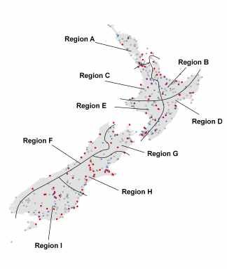
Figure 3. New Zealand’s 9 meteorological regions showing: • air temperature observation
stations; • stations meeting the selection criteria (station open between 1970-2008
with > 60 percent minimum air temperature records complete); • earth
temperature observations stations.
2.3.1 Quality control
An automated and objective quality control procedure was devised to screen station
level air temperature observations for potential errors (Figure 4), with the aim of
identifying and removing observations that would make the final analysis of frost
trends suspect. Quality control of climate time series for trend and other analyses can
take many forms (Peterson et al 1998): direct methods that rely on metadata; manual
Recent frost trends for New Zealand 8inspection; internal consistency testing that rely on statistical analysis; through to
external verification that compare series with an independent set.
Homogeneity and
CLIDB consistency testing
station series
remove suspect quality data
vcsn series
Bias correction
patch station series
data for analysis
Figure 4. Quality control and patching procedure used to build the minimum air
temperature dataset.
Five levels of quality screening are used in this study based on different approaches to
homogeneity and consistency testing. They were adapted for use in this study from
methods described by Thompson (1984), Rhodes and Salinger (1993), Alexandersson
and Morberg (1997), Brunet et al (2002) and the review of Peterson et al. (1998). The
five tests implemented are:
1. Suspect detection: suspects are those observations greater than 3.5 standard
deviations away from the monthly mean.
2. Internal consistency: observations failing the internal consistency tests are those
where the change from the previous observation is greater than 3.5 standard deviations
from the mean monthly change.
3. External homogeneity: Observations that fail the external homogeneity test have a
Z series deviation greater than 1.5 standard deviations from the monthly mean. The Z
series is based on a modification of the Standard Homogeneity Test (Alexanderson
1996), and are anomalies (between the observed and a reference set), normalised by
Recent frost trends for New Zealand 9seasonal and total variance. For the external homogeneity test the reference set is the
distance weighted mean of the three closest stations.
4. External homogeneity (vcs): this test repeats the Z score procedure and uses the
same criteria described for 3, but the reference set is taken as a distance weighted
mean of the VCSN time series across on a 5-by 5 grid box (25km2) over the
observation station.
5. Internal homogeneity (mean): this test repeats the procedure used in 3 and 4, but
uses the internal seasonal mean as the reference series.
Examples of two time series screened using these tests are in Figure 5. Both time
series have been modified to illustrate a range of potential problems, such as break
points, systematic shifts and changes in variance. The original signal for the station is
from 1982-2008. Both series have been infilled (prior to 1982) with a biased data
series using station observations taken upslope from this site. The period from 1991-
1995 in series A has been shifted by subtracting 1.5°C to introduce an unusual shift
with two definite breakpoints. The period 1990-2008 in series B has a negative
exponential trend imposed.
The symbols in the figures identify which observations fail a particular screening test.
As shown the tests clearly identified suspect data introduced into the series. The
external homogeneity tests identified both the artificial bias and in filled elements of
the series in Figure 3a. In Figure 3b the homogeneity tests identified multiple break
points, including those associated with the introduced negative exponential trend. In
both of these examples, a small number of observations failed the internal consistency
test, while very few failed the suspect detection test.
Recent frost trends for New Zealand 10a
b
Figure 5. Examples of time series screened using the homogeneity and consistency testing
procedure.
The quality control procedure was applied to both the air temperature and earth
temperature station data sourced from CLIDB. The number of suspect observations
identified is summarised at the regional and national level in Table 2. Typically
around 15-20 percent of observations were suspect for air temperature (with some
sites as little as 2-3%). There were more quality concerns in the earth temperature data
with around 30 percent of observations identified on average. For the air temperature
data the suspect observations were removed and replaced with bias corrected VCSN
series (described below).
Recent frost trends for New Zealand 11Table 2. National and regional summary of percent observations removed in quality
control.
Minimum air temperature Minimum earth temperature
Mean Max Min Mean Max Min
A 17.1 39.5 4.3 34 48.9 10.2
B 13.6 42.1 5.1 23.1 45.8 15.2
C 25.2 39.1 8.3 34.2 51.1 9.1
D 16.8 35.1 5.3 19.9 39.5 5.8
F 22.9 39.3 2.3 35.7 43.5 4.3
G 20.0 37.0 9.2 31.1 39.1 6.7
H 12.1 35.9 4.4 34.2 41.8 8.9
I 20.2 41.4 2.1 34.3 45.2 9.1
J 17.7 41.4 2.9 23.4 54.1 12.6
National 18.4 39.0 4.9 30.0 45.4 9.1
2.3.2 Bias correction for patching
The bias correction procedure used for the VCSN is based on methods described by
Ines and Hansen (2006) for correcting daily time series derived from global and
regional models for use in crop simulation. It involves truncating the cumulative
distribution function of the VCSN series to the cumulative distribution function of the
observed series, where:
P(n ) = V(n ) × a (n )
a(n ) ≅ A where V .cdf = V(n ) Equation 1
O.cdf
A=
V .cdf
where P is the patch series on day n, V is the virtual climate station observation, and a
is an adjustment factor taken form the adjustment vector A, where V corresponds to
the VCSN cumulative distribution function (V.cdf). O.cdf is the observed cumulative
distribution function for data where data flagged in quality control have been
removed. The bias corrected VCSN data is then used to patch missing data or
observations that had been removed in quality control.
Recent frost trends for New Zealand 12A cross validation was undertaken by partitioning the VCSN and station data into
fitting and evaluation subsets, where the former is used to determine the adjustment
vector A. Data from the evaluation subset is used to compare the untreated and bias
corrected VCSN data by correlation with the observed station data. The results of the
cross validation are shown in Table 3, where generally the bias correction yielded
higher correlations across all the meteorological regions.
Table 3. Summary of cross validation results (correlation coefficients) for the bias
correction procedure.
Region
A B C D E F G H I
VCSN 0.52 0.47 0.57 0.46 0.49 0.56 0.60 0.40 0.52
Bias corrected VCSN 0.78 0.76 0.75 0.71 0.79 0.83 0.76 0.72 0.89
2.4 Frost trend analyses
A range of methods can be used to detect the presence, strength and statistical
significance of trends in climate time series. Linear models can be fitted using
parametric (least squares regression) and non-parametric (for example pair wise slope)
methods. Polynomials and auto regressive moving average models (ARMA) can also
be considered if the series is non-monotonic. Extreme value analysis can be used to
examine trends in rare events such as heat waves. Non linear time series analysis
methods are also used for higher order problems, for example decomposition of series
to examine non-stationary components (example Figure 2). Common methods used to
detect and estimate the strength of trends in climate series are the Spearman Rank
Correlation Coefficient, the two sided Mann-Kendall test which is non parametric and
the Student t-test.
Trend detection in this study is carried out in a relatively straight forward way, using
ordinary least squares linear regression. This is an appropriate method for the problem
and level of analysis required in an initial study of trends, given the assumptions that
the relatively short series (36 years) is monotonic and the metrics analysed are
normally distributed. The slope parameter (trend) of the fitted linear model is
obtained for a number of metrics describing frost risk (detailed below), and reported
along with the F ratio and p value which characterise the strength of the linear fit to
the underlying data.
Recent frost trends for New Zealand 13A number of metrics are used to characterise frost risk and intensity that aggregate
occurrence either in space or time so as to be suitable for characterising climatology.
The following describes the general approach to the calculations, while the full range
implemented in this study is listed in Table 4.
The frequency of frost is calculated by determining the number of days in each year
minimum air temperature is below a critical threshold:
if O(n ) = T(n ) f (n ) = 1
Equation 2
else f (n ) = 0
F(Y ) =
∑ Y
f
∑ Y
n
where O are observed minimum air temperatures on day n. T is the critical threshold in
this case 0°C. f is a frost score being either zero for no frost or one for a frost day F is
the frost frequency in year Y. Growing season (September-April) and monthly
(excluding summer) analyses are undertaken by sub setting the observations to the
relevant time period each year. Thus Equation 2 is the total number of meteorological
frost days in a prescribed period divided by the total number of days in that period.
A metric describing the average temperature of meteorological frosts when they
occur was also calculated. Mean frost temperature (FT) for the year (Y) is taken as:
FT(Y ) =
∑ v( ) Y
where v (Y ) = O(Y ) ≤ T
∑ n(v( ) )
Equation 3
Y
where v are air temperature observations (O) that are equal or less than the critical
threshold T (0°C). n denotes the number of observation for v. Thus Equation 3 is the
average temperature of observations for a specified time period (in this case a year)
when temperatures are below 0°C.
The first frost day (S) each year (Y) is determined as:
S (Y ) = min (Fd (Y ) ) where Fd (Y ) ≅ doy ≅ O(Y ) ≤ T Equation 4
where Fd is the day of the Julian year (doy) that air temperatures are below a critical
threshold T (0°C). The last frost day (E) is taken as the maximum of Fd, while the
length of frost window L is E-S. Thus Equation 4 defines the first and last recorded
frost for a given year or season.
Recent frost trends for New Zealand 14National and regional composite time series are also produced by aggregating across
a meteorological zone, for example frost frequency is calculated as:
if O(r ,n ) ≤ T(n ) f (n,r ) = 1
Equation 5
else f ( n ,r ) = 0
FR(Y ) =
∑ Y ,r
f
∑ Y ,r
n
where r is the meteorological region (A-I, see Figure 1) and FR is the regionally
aggregated frost frequency. All other procedures are the same as for Equation 2.
Regional aggregation for mean air temperature, frost intensity and the first or last frost
dates differs in that the mean across the meteorological region is taken.
Table 4. Frost risk analyses undertaken in this study. Growing season period is October-
April. N is national composite, R is regional composite, S is station level analysis.
Indicator Units Annual Growing Monthly Scale
season
Frost frequency Probability/time * * * N,R,S
period
Or Days/time
period
Frost temperature Mean °C * * * R,S
First Frost Julian day * R
Last frost Julian day * R
Frost window Days * R
length
Minimum Mean °C * * R
temperature
Earth temperature Mean °C * * R
Recent frost trends for New Zealand 152.5 Spatial analysis
Two strategies are pursued for spatial analysis to address perceived limitations in the
sample of data: either its quality through time through time or across the country.
2.5.1 Calculate then interpolate
Station level trends are interpolated using a bi-variate thin plate smoothing spline from
the ANUSPLIN package (Hutchinson 1995, 1998a, 1998b). This strategy is pursues
to ensure that the quality of data is assured through time, but the approach does not
yield a large spatial sample for modelling. The general objective when fitting a spatial
interpolation function to sparse data is to find an appropriate balance between signal
and noise, thereby finding information about spatial variability at a broad scale while
not over or under fitting to the data at the individual site. In the thin plate spline this is
governed by selection of the smoothing parameter. The technical details of the spatial
analysis are as follows:
• all fitted spline surfaces were realised at a 5km2 resolution;
• all fitted spline functions were of second order
• for frost frequency analyses the most appropriate surfaces were obtained by a
square root transformation of the data, and estimating the smoothing
parameter by minimising the Generalised Cross Validation (GCV);
• for frost intensity analyses no transformation was required and minimising
GCV yielded an appropriate fit;
• for all trend analyses the data were truncated to a 1:5 range, a logit
transformation applied and the signal to noise ratio of 1:1 used;
• data for frost intensity trends was too sparse for valid surface fitting, so no
results are presented for this variable.
• in some cases individual station results were found to have high leverage, and
were removed from the data set. The influence of this procedure is shown in
Figure 6, where data from Dunedin Aerodrome is removed to provide a more
appropriate surface given the underlying data for mean annual frost frequency.
Recent frost trends for New Zealand 162.5.2 Interpolate then calculate
The metrics and approaches to trend fitting described in section 2.3 are fitted to
minimum temperature on a grid-by-grid basis for the VCSN network. There are some
questions about the strength of trends detected in this approach because of known
biases in the current data, for example because of poor sampling in the high altitude
zones it is known that above snowline temperatures have a warm bias (pers comm.
Tait 2009). In the lower lying and upland regions of the country, the sampling is more
comprehensive and independent validation demonstrates no discernable bias outside
of expected measurement error. While bias problems exist, this approach provides an
improved representation of the spatial variability across New Zealand, particularly the
role of the landscape in controlling trends. This is because the VCSN minimum
temperature set is based on all available observations from 1972-2008 and uses a three
dimensional spline providing additional support from digital elevation model.
High leverage data included High leverage data removed
Figure 6. Effect of removing high leverage stations from the interpolation of mean annual
frost frequency.
Recent frost trends for New Zealand 173. Results
3.1 National composite analysis
The national composite analysis (Figure 7) shows an overall decrease in frost
probability for the period 1972-2008 (-0.003 probability/decade), with corresponding
increases in frost temperature (+0.02°C/decade) and minimum temperature
(+0.07°C/decade). This equates to an on average decline of around 1 frost day per
decade. All the trends were significant at the 5 per cent confidence level. As illustrated
by the cumulative distribution plot (CDF) in Figure 8 approximately 70 percent of
stations had negative trends, ranging from -0.1 to -1.5 days per decade.
Annual Growing season
Figure 7. National composite annual and growing season frost probability, intensity and
minimum temperature trends.
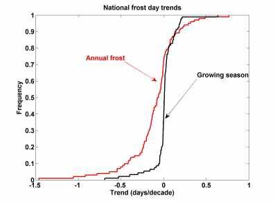
Recent frost trends for New Zealand 18When examined for the growing season the trends are not as strong (Figure 7) nor
were they statistically significant at the five or ten percent confidence levels. The sign
of the frost probability trend also changes from a negative trend for the annual time
period to a very weak positive trend (+0.0002 P/decade) for the growing seasonl time
period (Figure 7, right hand side). This result is also evident in Figure 8, where the
dominant signal in the national composite is a neutral trend, with between 50-60
percent of stations having no change in the number of frost days for 1972-2008.
Figure 8. Empirical cumulative distribution functions showing the frequency of station
level trends for the growing season (October-April) and annual time periods.
3.2 Regional composite analysis
The overall direction of trends found for the national composite analysis were also
found for the regional analysis—frost risk was found to be decreasing in most regions
and minimum temperature and frost intensity were found to be increasing for all
regions for the annual time period. The exception to this result was for
Meteorological Region E where a positive trend in frost risk was found. All the
trends reported for the annual time period at the regional level were significant to at
least the 10 percent confidence level (Table 5).
Recent frost trends for New Zealand 19Table 5. Regional composite trends (unit/decade). Numbers in bracket are F test
probabilities. * is significant where P>0.1 and ** is significant where P>0.05.
Frost risk (P) Frost temperature Minimum temperature
(°°C) (°°C)
Annual
Region A -0.0008 (3.0)* 0.12 (9.8) ** 0.2 (12.1)**
Region B -0.004 (8.3)** 0.009 (1.0)** 0.06 (1.0)*
Region C -0.003 (4.7)** 0.04(6.2)** 0.08 (1.8)*
Region D -0.0005 (2.2)* 0.06(12.1)** 0.04 (0.4)*
Region E 0.0004 (2.3)* 0.02(0.8)* 0.08 (1.7)*
Region F -0.003 (5.2)** 0.05 (2.2)* 0.09(2.3)*
Region G -0.011 (6.1)** 0.107(13.2)** 0.2 (12.0)**
Region H -0.004 (3.6)* 0.1 (12.5)** 0.04 (0.6)*
Region I -0.003 (3.1)** 0.01(2.1) 0.02 (0.2)
Growing season
Region A -0.00001(0.2) 0.07 (3.1)** 0.04 (1.7)*
Region B -0.0004 (0.7) 0.04 (4.2)** -0.03 (0.3)
Region C -0.0001 (0.03) 0.07 (3.5)** 0.05 (3.2)**
Region D 0.0005 (0.9) 0.07 (1.3)** -0.04(3.0)**
Region E 0.0005 (0.6) 0.05 (1.3) -0.07(3.0)**
Region F -0.0003 (0.1) 0.09 (4.1)** -0.04(2.6)
Region G -0.003 (12.4) 0.09 (4.3)** 0.03(1.3)
Region H -0.002 (1.03) 0.15 (12.1)** -0.01 (3.4)**
Region I 0.003 (2.1) -0.3 (3.1) -0.03 (2.1)
Like the national analysis the growing season time period did not have the same trend
direction and strength as the annual time period. None of the frost probability trends
were statistically significant for the seasonal analysis. However at this scale
differences between regions do emerge (Table 5). Regions D, E and H exhibited a
significant cooling trend in growing season minimum temperature of the order of -
0.03 °C/decade, B and F had negative trends that were not significant, and A, C and G
had a warming trend. Most of the regions had a significant positive growing season
frost temperature trend (warming), with the exception of region I.
Recent frost trends for New Zealand 203.3 Frost seasonality
Trends in dates defining the opening and closing of the frost season (as well as season
length) are in Table 6 for the regional scale of analysis. At this scale the reported
metric is the 5th percentile of opening frost date across the region and the closing date
the 95th percentile. For opening frost date both positive and negative trends were
detected but these were not statistically significant at either the 5 or 10 percent
confidence level , except for the positive trend in region A. All of the end of season
(last) frost day trends were positive (i.e. the last day was becoming later), with
significant trends found in regions C, D, E and I. Both positive and negative trends
were found for the season length, with the positive trends in regions D, E and I being
significant.
Table 6. Trends in frost start date, end date and season length for New Zealand
Meteorological regions. Start date is the 5th percentile of observations and end
date the 95th percentile. Numbers in brackets are F test probabilities. * is
significant where P>0.1 and ** is significant where P>0.05.
Region Mean (date) Trend (days/decade)
Start of frost season
A 10 June 6.5 (9.7)**
B 20 May 2.1 (1.7)
C 16 May 1.1 (0.5)
D 21 May 0.4 (0.06)
E 2 May -1.0 (0.3)
F 9 May 0.7 (0.1)
G 27 April -1.1 (0.5)
H 30 April 1.2 (0.5)
I 1 May -1.5 (1.3)
End of frost season
A 14 August 2.6 (0.67)
B 13 September 0.2 (0.01)
C 10 September 5.4 (5.5)**
D 17 September 6.0 (5.8)**
E 2 October 3.9 (2.2)*
F 24 September 2.2 (1.0)
G 1 October 0.5 (0.07)
H 11 October 0.7 (0.1)
I 23 September 4.0 (6.5)**
Length of frost season
A 65 -3.8 (1.2)
B 116 -2.3 (0.5)
C 118 4.2 (2.4)
D 119 5.6 (3.5)**
E 152 4.9 (2.1)*
F 138 1.5 (0.3)
G 157 0.5 (0.03)
H 163 -0.5 (0.05)
I 145 5.6 (7.5)**
Recent frost trends for New Zealand 213.4 Threshold sensitivities
To provide more information about the influence of the temperature threshold on the
results sensitivity analyses were undertaken at the national level. Figure 9 show
responses of the national average frost frequency, temperature and frost season length
trends to changes in the threshold between -2 and + 4 °C. The results show that trends
in frost frequency were not sensitive to the critical temperature used. As the critical
temperature selected becomes warmer the magnitude of the trend increases. A similar
result was also found for frost temperature, although there is a lot more irregularity in
the sensitivity tests, for example the large spike at -1.7 °C. For frost season length
changing the threshold results in a directional change in the national trend—it remains
neutral to positive (increasing seasonal length) up to a threshold around 0°C and
becomes negative (decreasing seasonal length) above this level. This result, and also
the irregularities in both frost temperature and frost season length are indicative of the
process control on these metrics—synoptic patterns have a greater influence on these
metrics when compared to frost frequency.
Figure 9. Sensitivity tests of the national mean trend to changes in the frost threshold.
3.5 Earth temperature
The earth temperature results are summarised for the regional level in Table 7. Similar
to the frost risk analysis, earth temperature trends exhibited region-to-region
variability in terms of their direction and strength. Significant positive (warming)
trends were detected for the annual period in regions A, B, and F. Positive trends were
also found for regions G and H but these were not significant at the 10 or 5 per cent
Recent frost trends for New Zealand 22confidence level. Negative (cooling) trends were detected in regions C and I, with the
F-test not significant. For the growing season analysis a weak negative (cooling) trend
was detected that were not statistically significant.
Table 7. Trends (units/decade) in annual and seasonal earth temperature. ( ) are F test
probabilities. * is significant where P>0.1. ** is significant where P>0.05.
Annual
Region A 0.01 (2.5)**
Region B 0.002 (10.5)**
Region C -0.0001(5.1)
Region D -0.001(5.3)
Region F 0.02(4.1)**
Region G 0.0081(1.2)
Region H 0.004 (0.3)
Region I -0.0008 (1.7)
Region J 0.02(4.9)**
Seasonal
Region A -0.003 (0.1)
Region B -0.005(1.6)
Region C -0.001(5.8)
Region D -0.008(4.4)
Region F -0.006(2.6)
Region G -0.006(2.9)
Region H -0.006(3.1)
Region I -0.007(3.7)
Region J -0.0004(4.2)
3.6 Spatial analysis
The spatial interpolation of station level results are provided as a series of national
maps in Appendix 2. The map of frost climatology (Appendix 2, Maps1-10)
highlights that the station data set used in this research was able to be used to build
interpolated surfaces broadly representing frost risk across the country. They reflect
the very broad landscape and coastal processes that control frost climatology. The
spatial distribution of frost risk produced in these maps is in broad agreement with the
frost climatology produced by Goulter (1981). However the data are not densely
Recent frost trends for New Zealand 23sampled and interpolation methods not sensitive enough to map the finer landscape
modification of frost which were detected in the Goulter study.
The key results for this work are the annual and seasonal frost risk analyses (Maps 11-
12, Appendix 2), also shown as Figure 10. This highlights a strong spatial signal in
direction of trends in frost risk across New Zealand found in this study. That is both
the negative and positive trends detected in the national composite analysis (section
3.1) are concentrated in regions. That is there appear to be more frosts in a few
regions than rather than a random distribution over the country. The spatial analysis
also re-enforce the results obtained in the composite analyses, that a clearer signal is
evident in the annual analysis compared with the seasonal analysis. The results also
provide a better examination of the spatial distribution of trends within New Zealand
than the regional composites which were structured according to pre defined zones.
The spatial analysis suggests that the increase in frost frequency (cooling) is
concentrated in two areas both on the eastern sea board of New Zealand. The first is
the south east of the North Island encompassing the agricultural zone in the
Wairarapa. The second is a larger zone on the south east of the South Island, from
Ashburton to Dunedin. Interpolated trends in these zones are strong (+0.2 to +0.3
°C/year). Strong negative trends in annual frost frequency (warming) are located in the
alpine regions of both islands.
Recent frost trends for New Zealand 24Figure 10. Interpolation of station level trends for seasonal (growing season) and annual
frost frequency.
Recent frost trends for New Zealand 25There was little spatial structure when frost frequency trends were interpolated at the
monthly level and the signal to noise set at half the number of data points (Maps 13-
20). This is evidence that the trend signal was relatively weak when examined at the
monthly time period, particularly for the late and early season months of April (Map
13) and November (Map 14). Similarly little coherent spatial structure was evident in
the interpolation of trends for the frost seasonality indices (maps not provided).
When the interpolate then calculate approach was used the same broad spatial
structure in frost trends was found (Figure 11, Map 31). The most pronounced positive
trends in frost frequency remain the region of the Wairarapa, and the area below
Ashburton on the South Island. Additional areas of moderate increases in frost
frequency were also detected using this approach, including a part of the Canturbury
plain, Nelson hinterland and western Southland on the South Island, and the
Ruaukumara Range on the North Island. The area of large positive decrease in frost
frequency centred on the Southern Alps and Tongariro—evident as a smooth region in
Figure 10—appears to be topographically controlled when this approach to spatial
analysis is used. The strength of the trend in the higher altitude zone should be
questioned because of known data availability limitations in these zones. Notably,
most of the remaining major agricultural regions exhibit a neutral to slightly negative
trend in frost frequency.
Importantly, an increase in frost frequency was detected in the Tasman and Nelson
hinterland districts using interpolate then calculate (Figure 11, Map 31), whereas when
trends were interpolated from individual stations this feature was smoothed and a
decreasing trend was found (Figure 10, Map 11). Closer inspection of the spatial
distribution of the station data used to produce Map 11 (Figure 6) highlights that in the
Nelson region the stations were located on the coast, and there is a poor sample in the
Tasman. It is likely that these sampling features have biased the fitted surface in these
regions for the calculate then interpolate approach. Hence, it is advised to give more
weight to the increasing frost frequency trend found by the interpolate than calculate
approach (Figure 11, Map 31) for the Tasman and Nelson districts. Further ratification
of these trends may be warranted by analysis of individual station series in these
districts.
It was also possible to examine if any spatial patterns were evident in the significance
tests of trends using the interpolate then calculate approach (Figure 12). Generally
areas that have been identified as being either strongly positive or negative in terms of
frost frequency trend were significant at either the 5 or 10 percent level, and there is a
degree of spatial coherence in these results.
Recent frost trends for New Zealand 26Figure 11. Frost trends detected when using the interpolate then calculate approach. Recent frost trends for New Zealand 27
Figure 12.           Significance test for frost frequency trends using the interpolate then calculate
                     approach.

Recent frost trends for New Zealand                                                                      28
4. Discussion
4.1 Interpretation
Interpretation of the results obtained in this study relies on understanding the different
scale of process that control frost in New Zealand. Detection of reduced frost
frequency at the national composite level and for the annual time period is consistent
with a decadal scale warming of the global atmosphere. The methodology underlying
the national composite analysis is well suited to detecting trends at these broad scales,
but not as sensitive to local scale variability. This is consistent with the results
obtained by Zheng et al (1997) and Salinger and Griffiths (2001), and also the global
level climate change reported by the IPCC (IPCC 2007).
As the time and spatial scales of the frost trend analyses became finer, the greater the
influence of inter annual, seasonal and weather processes. New Zealand’s maritime
climate has potential to modify the overall global signal, and as found in this study, it
is plausible that regional and sub regional trends can run counter to the direction of
those detected at the national and global scale. Regional variability of this type is also
evident when global climate change projections are downscaled for New Zealand
(Mullan et al. 2007). Frost occurrence at the regional and growing seasonl level is
largely controlled by the stability of weather systems, and trends driven by the
persistence of certain weather types. It is possible to form a starting hypothesis about
the process controls on the results, as the spatial distribution of annual and growing
seasonstation trends is consistent with a more persistent southerly flow and north
westerly winter flow influencing New Zealand (pers comm. Mullan 2009).
It is also important to recognise the potential drivers of frost influencing the results
found at the finer monthly time scale and for the frost season indices. At this level the
occurrence of frost is more strongly influenced by the nature of individual weather
events, rather than broader signals from atmospheric warming and circulation
(weather type persistence). This is particularly the case for the occurrence of out of
season frosts (April and November analyses)—the empirical results in this study
showed that no linear trend could be detected at the monthly level and that the thirty
year time series have an almost random like nature. At the empirical level, the frost
indices at these finer time scales and outside of the higher elevation zones can be
considered as being more responsive to the noise driven by weather rather than the
signal driven by a shift in large scale climate forcing.
As described in the introductory sections, the study has been confined to one climate
period 1972-2008, where there is sufficient data to examine the regional variation in
Recent frost trends for New Zealand 29frost occurrence across New Zealand. Most of this time slice was in one positive
phase of the Interdecadal Pacific Oscillation, which has been observed in long run
series and identified as a significant source of climate variation at decadal time scales
throughout the South West Pacific (Salinger et al. 2001, Folland et al 2002). It was
not possible with the 1972-2008 time series and methods used here to estimate the
relative contribution of the decadal and longer term global signals to the trends
reported, particularly if the spatial distribution found is part of decadal or longer term
variability. Hence, it is plausible, given a decadal scale oscillation in the Pacific’s
climate, that the magnitude and or spatial pattern in the direction of the trends detected
in this study could change in the future despite the expected continuation and
strengthening of global scale warming.
For primary production, frost is both a climatic feature and weather event that can be
managed to some extent, depending upon the viability of mitigation options. This
study detected a trend that is consistent with global warming, so it might be tempting
to conclude that it is possible to lower frost mitigation standards and reduce costs in
the coming years. However, extension of the national trend found in this study to form
such a conclusion is invalid. The regional variability created by New Zealand’s
maritime climate, means that in some regions frost trends may be increasing rather
than decreasing on decadal time scales in a background of global warming. On the
shoulders of the growing season, where a frost event has potentially severe impacts
because of increased exposure, frosts are strongly controlled by the weather and these
show little persistent signal through time. For management of production systems in
the next decade, damaging frost should continue to be considered a natural hazard,
where diligent monitoring of day to day weather information and matching actions to
long term climatic frequency analysis is the best pragmatic approach.
4.2 Limitations
The analyses undertaken in this study were limited by the amount of data available,
both across New Zealand and through time. Additional series through time would
allow a more thorough examination of decadal scale influences such as the
Interdecadal Pacific Oscillation or changes in the persistence of Kidson weather
regimes on trends and support alternative analytical methods (see below). This has
already been completed to some at the empirical level in the studies of Zheng et al
(1999), Salinger and Griffith (2001) and Withers et al (2007), but more work is
warranted in terms of attribution of trends. While some interpretation about the
consistency of the detected trends with climate processes has been made, there was
insufficient observation series to complete a formal attribution study.
Recent frost trends for New Zealand 30Similarly, increasing the number of sites across New Zealand would build more
confidence in the spatial modelling of trends. It is important not to over interpret fine
level geographic detail from the maps produced in the appendices and in Figure 10
and Figure 11—that is, it is not possible to identify trends at specific locations from
these maps. Given the data and methods used, the maps convey the broad regional
structure of frost occurrence and trends, but there is insufficient network to support
detailed landscape scale spatial modelling of frosts. Hence, localised variability that
producers are fully aware of, such as the gradient in frost frequency experienced
across a valley, or from one paddock to the next, are not evident in the analysis.
Given the length of the series available and scope of the study, a choice was made to
use linear least squares regression techniques to detect trends. Other non-linear
methods may have provided different insights, particularly when examining longer run
series and studying the contribution of decadal processes. There is also scientific
debate surrounding the usefulness of significance testing in analysing climate trends.
For example Nicholls et al. (2000) advises that a trend should not be dismissed out of
hand if it does not pass a significance test, particularly if there is strong confirmatory
evidence from other data and a process explanation. Similarly it is wise to question a
trend even if it is statistically significant and there are no reasonable process
explanations or confirmatory analyses.
The analyses pursued here use a meteorological definition of frost, simplifying its
occurrence definition so that its implied risk may be assessed with standard Stevenson
screen observations. As discussed in the introductory sections, the meteorological
definition of a frost does not always correlate directly with an event that causes
damage to crops and trees having a production impact, and is therefore only a partial
measure of frost risk for the primary industries. Full frost risk analysis is usually only
possible at a very localised scale, with more refined data and information about the
sensitivity of a given crop and variety to freezing. It was not possible to pursue this
level of detail and provide a national coverage for this study.
4.3 Further work
This initial study of recent frost trends highlights a number of areas that may be
addressed by further research. Of particular importance is understanding the regional
direction of trends in frost risk under a changing climate through formal attribution
studies of both the global climate change signal and its modification by synoptic
processes. Further ratification of the trends detected in this study is required using
improved data sets, supplemented with output from climate models and remote
sensing. We advise that this is necessary step, along with formal attribution, before
Recent frost trends for New Zealand 31You can also read